Tracking the Orbital and Super-orbital Periods of SMC X-1

Abstract

The High Mass X-ray Binary (HMXB) SMC X-1 demonstrates an orbital variation of $\sim$3.89 days and a super-orbital variation with an average length of $\sim$55 days. As we show here, however, the length of the super-orbital cycle varies by almost a factor of two, even across adjacent cycles. To study both the orbital and super-orbital variation we utilize lightcurves from the Rossi X-ray Timing Explorer All Sky Monitor (RXTE-ASM). We employ the orbital ephemeris from Wojdowski et al. (1998) to obtain the average orbital profile, and we show that this profile exhibits complex modulation during non-eclipse phases. Additionally, a very interesting “bounceback” in X-ray count rate is seen during mid-orbital eclipse phases, with a softening of the emission during these periods. This bounceback has not been previously identified in pointed observations. We then define a super-orbital ephemeris (the phase of the super-orbital cycle as a function of date) based on the ASM lightcurve and analyze the trend and distribution of super-orbital cycle lengths. SMC X-1 exhibits a bimodal distribution of these lengths, similar to what has been observed in other systems (e.g., Her X-1), but with more dramatic changes in cycle length. There is some hint, but not conclusive evidence, for a dependence of the super-orbital cycle length upon the underlying orbital period, as has been observed previously for Her X-1 and Cyg X-2. Using our super-orbital ephemeris we are also able to create an average super-orbital profile over the 71 observed cycles, for which we witness overall hardening of the spectrum during low count rate times. We combine the orbital and super-orbital ephemerides to study the correlation between the orbital and super-orbital variations in the system, but find that the ASM lightcurve provides insufficient statistics to draw any definitive conclusions on possible correlations.

1. Introduction

SMC X-1, first discovered with Uhuru observations (Leong et al. 1971), is a High Mass X-ray Binary (HMXB) consisting of a neutron star (an X-ray pulsar with 0.71 s period; Lucke et al. 1976) and a young B0 supergiant companion (Webster et al. 1972; Liller 1973). An accretion disk is formed around the neutron star, likely partly via wind-fed accretion where a strong stellar wind from the companion star blows mass beyond its Roche Lobe radius and into the gravitational influence of the neutron star. Our view of this system is at high inclination, as we witness X-ray eclipses of the neutron star and disk by the companion star once every orbital period (Schreier et al. 1972).

These previous studies of the SMC X-1 system measured the orbital period to be approximately 3.892 days. As has been observed in similar HMXB systems, SMC X-1 also exhibits a long time scale ($\approx 60$ days) super-orbital variation in its X-ray lightcurve (Gruber & Rothschild 1984). Unlike the super-orbital variation in systems such as Her X-1 (Tananbaum et al. 1972), which has a relatively predictable 35 day period length (Staubert et al. 1983), the super-orbital cycle length in SMC X-1 is highly variable and follows no obvious pattern (Gruber & Rothschild 1984; Wojdowski et al. 1998). As we elaborate upon further below, lengths of the super-orbital cycles in SMC X-1 can vary by up to a factor of two.

Accretion disk systems with super-orbital variations have been explained with warped disks, seen close to edge-on such that the warp partially obscures our view of the X-ray source (Katz 1973). Such warps are possibly due to an instability driven in the outer disk by radiation from the central X-ray source (Petterson 1977; Pringle 1996; Maloney et al. 1996), or a number of other mechanisms (see Caproni et al. 2006, for a review). Wojdowski et al. (1998) suggested that the super-orbital variation seen in SMC X-1 is indeed due to obscuration by such a warped disk, as opposed to intrinsic flux variations, since the flux and spectrum during orbital eclipse are fairly insensitive to whether the system is in a ‘low’ or ‘high’ state of the super-orbital variation.

It also has been suggested that SMC X-1 possibly has multiple warp modes in its accretion disk in order to account for the wide variation in super-orbital cycle length (Clarkson et al. 2003). For radiatively driven warps, theoretical studies show a number of possible “branches” of mode solutions that encompass both prograde and retrograde, as well as stable and damped warps (Wijers & Pringle 1999; Ogilvie & Dubus 2001). On the other hand, observational evidence has been found in similar systems suggesting interaction between the super-orbital variations and the orbital period or some other underlying ‘fundamental clock’ (Boyd & Smale 2004). Such systems have been shown, in some cases, to have super-orbital cycle lengths equal to integer or half-integer multiples of an underlying clock, which in the case of Cyg X-2 is the orbital period, while in the case of LMC X-3 and Cyg X-3 is not simply related to any known dynamical period in the system (Boyd & Smale 2004). (The super-orbital variations in LMC X-3, however, are likely due to flux variations rather than obscuration; Wilms et al. 2001.) In Her X-1 the super-orbital cycle length mainly exhibits three values randomly, each differing only by half the orbital period (Staubert et al. 1983; Still & Boyd 2004; Klochkov et al. 2006).

In this work we use data from the All Sky Monitor (ASM) on board the Rossi X-ray Timing Explorer (RXTE) to make a comprehensive study of the long term X-ray light curve of SMC X-1. We study and characterize both the average orbital variation and super-orbital variations in this system. The outline of our paper is as follows. In §2 we discuss the extraction and reduction of the ASM data. We first use these data to characterize the average X-ray properties of the orbital period (§3). Next, in §4 we discuss how we define the ephemeris for the super-orbital variations, and then in §5 we present their average X-ray properties. In §6 we consider jointly the average X-ray properties of the orbital and super-orbital variations. Finally, we summarize our conclusions and make comparisons to other systems, such as Her X-1, in §7.

2. ASM Data Reduction

The ASM consists of three scanning shadow cameras, each equipped with a position sensitive proportional counter that views the sky through a set of slits to measure the relative intensities and positions of X-ray sources in the sky (Levine et al. 1996). The detector operates by comparing observations of intensities in any given area of the sky to a catalog of known X-ray sources to obtain a lightcurve (on time scales as short as 90 s) for each target in the field of view. The ASM records data in three different energy channels. Channels one, two and three are sensitive to X-rays of energy 1.5–3 keV, 3–5 keV and 5–12 keV, respectively.

We obtained definitive lightcurves for SMC X-1 from the ASM source catalog at the NASA RXTE website, and analyzed data beginning MJD 50088.4 and ending 54083.8. As mentioned previously, the ASM data consists of a least-squares fit to the sky’s modeled X-ray spectrum for all the known sources within its field of view. For this reason the count rate (cps) measurements from the satellite will occasionally fall below zero when the target source counts are lower than the difference between the expected background and the actual background; we have not excluded such negative counts from our extracted lightcurves.

Our analysis was performed using ISIS version 1.4.2-5 (Houck & Denicola 2000), using custom scripts written in S-lang (the scripting language embedded within ISIS), as well as routines publicly available from the S-lang/ISIS Timing Analysis Routines (SITAR). Using these routines to read the ASM data, we only retained data points where the ASM solution had a maximum $\chi^{2}$-value of $<1.5$. Before beginning any analysis, we performed a barycenter correction on the lightcurve to account for the movement of the satellite within the Earth-Sun system.

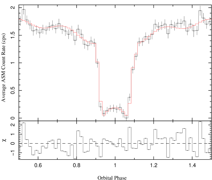
Figure 1.— The ASM lightcurve of SMC X-1 folded on the orbital period, fit with a 10 parameter empirical model. Error bars are $1\,\sigma$, and are derived from the standard deviation of the mean rate in each bin. The bounceback feature is clearly visible between phases .875 and 1.025

The ISIS define_counts function allows arbitrary arrays of lo/hi bin, value per bin, and error on that value to be registered as a fittable data set, with presumed diagonal response matrix and unity effective area. We used this functionality to register the folded ASM lightcurves of §3 and §4 for fitting, and used combinations of custom defined S-lang functions to fit these data. When it was necessary to fit a function to $(x,y)$ pairs rather than histogram data sets (see §4), we used the ISIS function fit_array, which takes as input arrays of $x$- and $y$-values, the relative weights of the data points, parameter initial values and limits, and a reference to a single user-defined S-lang fit function.

3. Folding the Orbital Period

Our first step in characterizing the behavior of SMC X-1 was to search the ASM lightcurve for evidence of the aforementioned periodicities. Using a Lomb-Scargle periodogram (Lomb 1976; Scargle 1982) we were able to detect both a 55 day period (the average length of the super-orbital cycles; see §4) as well as a period of approximately 3.89 days (i.e., the orbital period). These findings correspond to previous observations of the source (Wojdowski et al. 1998; Wen et al. 2006). We obtained an orbital ephemeris for the source from Wojdowski et al. (1998), which was defined in terms of the initial observation time, the period and the period first derivative. Using this ephemeris with the SITAR routine sitar_pfold_rate, we folded the ASM lightcurve into 60 phase bins, as shown in Fig. 1.

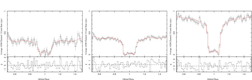
Figure 2.— Folded orbital profiles of the three ASM energy channels, from left to right 1.5–3, 3–5 and 5–12 keV. Both the bounceback and complex orbital modulation are more prominent in the lower energy channels.

We had originally thought to search for improvements on the Wojdowski et al. ephemeris by detecting a drift in the zero point of orbital phase (even relative to the known orbital period derivative from that work) over the 11 years of ASM data we analyzed, but found that any possible drift in the ephemeris was well within the observational errors of the ASM. The Wojdowski et al. (1998) ephemeris remains accurate.

Using the folded lightcurve, we were able to observe several features of the orbital profile. The most interesting of these features is a “bounceback” phenomenon occurring during the eclipse. Because we are observing the system at high inclination, we expect to have few to no counts during the eclipse phases, when the companion star obscures the line of sight between the satellite and the neutron star-disk system. Surprisingly, we observe the low counts expected on either side of the eclipse, but witness a small rise and fall of counts during the mid-eclipse phases. We will henceforth refer to this region of recovering count rate as the “bounceback.” Another interesting feature is a complex modulation, modeled below as sinusoidal, that occurs throughout the signal profile, and that is very visible during the non-eclipse phases.

We were able to obtain a fit to describe these features of the orbital profile using a ten-parameter empirical function. Our final model was obtained as follows. We modeled the bounceback feature in the center of the eclipse with a parabola. Allowing a free parameter for the magnitude of the curvature, which could range to any real value (positive or negative), we noted that the curvature was fit to positive values in all channels. Eclipse ingress and egress were modeled by linear functions, dropping from/rising to a constant value outside of eclipse. We multiplied the entire function by a sine wave plus a constant to account for the modulation observed in the profile, and subtracted a Gaussian from the center to account for a broader component of the eclipse, possibly due to partial obscuration of potentially extended X-ray emission by the companion star and/or accretion stream. The center of the Gaussian and parabola were fixed at 1, while the sinewave frequency was fixed at an integer or half-integer multiple of the inverse orbital period. We attempted the fit with several different integer and half-integer values and used the frequency with the lowest $\chi^{2}$ in our final fit function. It is interesting to note that the best fit was obtained modeling the modulation with a sine wave of frequency 4 (in units of the inverse orbital period), implying a complex disk warp structure.

Aside from the amplitude of the constant, amplitude and phase of the sine wave, and area and standard deviation of the Gaussian, free parameters also included widths for each of the regions: the eclipse, the ingress, and the egress. The folded data, fit and residuals are plotted in Fig. 1, and the parameters are given in Table 1. This model, as well as other non-standard models used for fitting in this paper, were written by the authors and can be made available upon request.

Once a successful model was obtained we were able to utilize it to fit orbital profiles to each of the individual energy channels of the ASM data (1.5–3, 3–5, and 5–12 keV) and compare the normalizations of features of the system in different energy ranges. Fig. 2 shows profiles and fits in each of these three energy channels, and the fit parameters are also presented in Table 1. In general we found that the lightcurve count rate was dominated by the high energy portion of the spectrum. As expected we also found more modulation in the low energy channels than in the high, likely due to preferential absorption of low energy X-rays, and also possibly due to the relative sizes of the sources of high and low energy X-rays.

Due to count rate uncertainties, it is not initially clear whether or not the bounceback and sinusoidal variation are significant, real features of the orbital profile. In order to further explore the significance of the bounceback, we performed fits of the orbital profile without the parabolic term, resulting in a $\Delta\chi^{2}$ from the fits to the full model described above of 14.1 in the summed channel fit and 1.0, 2.0 and 10.0 in fits of the first, second and third channels respectively. We also performed the orbital profile fits without the sinusoidal modulation, which resulted in a $\Delta\chi^{2}$ of 13.2 in the summed channel fit and 5.4, 7.9 and 2.3 in the fits of the first second and third channels respectively from the $\chi^{2}$-values obtained using the full model. The statistics are not good enough to allow study of the bounceback or the sinusoidal modulation in individual periods. The bounceback is not clearly exhibited in averaging of most short portions of the lightcurve (i.e., only a few orbital periods) but can only be found with the statistics provided by long averaging times. A more thorough understanding of the bounceback would require better statistics than presently available from the ASM data.

Table 1Orbital Profile: Constant*((1.0+Sinewave)*Orbit+Gauss)

ASM	$\chi^{2}_{red}$	Constant	Sinewave		Orbit					Gauss
Channel	(50 DoF)		Norm	Phase	Lwidth	Rwidth	Cwidth	Height	PNorm	Area	Sigma
1+2+3	1.00	$1.74^{+0.02}_{-0.02}$	$0.036^{+0.016}_{-0.014}$	$0.72^{+0.07}_{-0.06}$	$0.100^{+0.001}_{-0.005}$	$0.103^{+0.005}_{-0.003}$	$0.134^{+0.001}_{-0.001}$	$0.77^{+0.02}_{-0.01}$	$0.10^{+0.03}_{-0.03}$	$-6.4^{+0.4}_{-0.4}$	$0.18^{+0.01}_{-0.02}$
1	0.95	$0.40^{+0.05}_{-0.07}$	$0.063^{+0.038}_{-0.047}$	$0.68^{+0.07}_{-0.06}$	$0.117^{+0.017}_{-0.015}$	$0.112^{+0.013}_{-0.019}$	$0.122^{+0.878}_{-0.025}$	$0.73^{+0.21}_{-0.33}$	$0.17^{+0.17}_{-0.47}$	$-17.5^{+7.5}_{-2.5}$	$0.41^{+0.25}_{-0.21}$
2	0.78	$0.39^{+.04}_{-.01}$	$0.048^{+0.026}_{-0.027}$	$0.78^{+0.09}_{-0.09}$	$0.100^{+0.006}_{-0.015}$	$0.106^{+0.007}_{-0.018}$	$0.140^{+0.860}_{-0.009}$	$0.87^{+0.11}_{-0.18}$	$0.12^{+0.14}_{-0.09}$	$-4.9^{+1.8}_{-2.3}$	$0.17^{+0.17}_{-0.06}$
3	1.14	$0.86^{+0.03}_{-0.01}$	$0.018^{+0.018}_{-0.018}$	$0.74^{+0.26}_{-0.74}$	$0.095^{+0.002}_{-0.004}$	$0.100^{+0.006}_{-0.001}$	$0.133^{+0.007}_{-0.005}$	$0.74^{+0.06}_{-0.08}$	$0.09^{+0.07}_{-0.07}$	$-6.3^{+1.2}_{-2.1}$	$0.17^{+0.06}_{-0.04}$

Note. — ORBIT function parameters: Lwidth=width of the eclipse ingress, Cwidth=width of the eclipse from low point on the left of the bounceback to low point on the right of the bounceback, Rwidth=width of eclipse egress. Height=Distance from lowest point in the eclipse to the constant in non-eclipse phases. PNorm=Height of the parabola fit in the bounceback (center of the eclipse) region. In Lwidth and Rwidth regions the profile was modeled with a linear function and in the Cwidth region the profile was modelled as a parabola. Center of Orbit model and Gauss were frozen at phase=1 and the sinewave frequency was frozen at f=4 (Orbital Period)^-1. Error bars are 90% confidence levels.

Figure 3.— Top: The orbital-folded color lightcurve, exhibiting overall hard X-ray dominated emission with softer X-ray emission in the bounceback region. Error bars are are $1\,\sigma$ error bars. Bottom: The same folded lightcurve as above; however, each energy channel lightcurve was systematically shifted upward by 0.05 cps.

In order to get a more quantitative idea of the energy distribution of the emission, we created a folded color lightcurve, where we defined the color, $C$, as

$$C=\frac{{\rm ch}1-{\rm ch}3}{{\rm ch}1+{\rm ch}3}$$ (1)

Here ${\rm ch}1$ is the count rate measured in ASM channel one, and ${\rm ch}3$ is the count rate measured in channel three. Thus if the emission at a certain phase is dominated by hard X-rays, then the value of the color will be negative, and if the emission is dominated by soft X-rays the color will be positive. The orbital phase-dependent color lightcurve (with 40 phase bins) is plotted in Fig. 3.

Overall the color lightcurve demonstrates that the source is relatively monochromatic and dominated, as observed in the channel fits, by hard X-ray emission. We did find that at the edges of the eclipse, where the source was being partially obscured by the companion star, that the X-ray emission possibly becomes much harder. This might be attributable to soft X-ray absorption from the outer atmosphere of the companion star; however, this region of the lightcurve is also where the average ${\rm ch}1$ lightcurve dips below 0. If we apply a systematic shift upward of 0.05 cps to each of the lightcurves, this hardening disappears, although the hardening remains a possibility within the uncertainties. On the other hand, the bounceback emission, in contrast to the emission in the rest of the orbital cycle, clearly becomes softer.

4. Defining the Super-Orbital Ephemeris

The inherent noise of the lightcurve and the highly variable nature of the super-orbital cycle length provided somewhat of a challenge as far as the definition of the super-orbital ephemeris (super- orbital phase to date correlation) was concerned. Here we wish to consider only variations on the longer super-orbital time scale, and not those produced by the orbital variations. We therefore removed points that fell within the eclipse of the neutron star by the companion from the lightcurve. Using our orbital fold, discussed in the previous section, we determined the orbital phases of the eclipse to lie between 0.85 and 1.15 (Fig. 1), and used the Wojdowski et al. (1998) ephemeris to calculate the time ranges during which these phases would occur. We then removed all ASM data points that fell within those ranges.

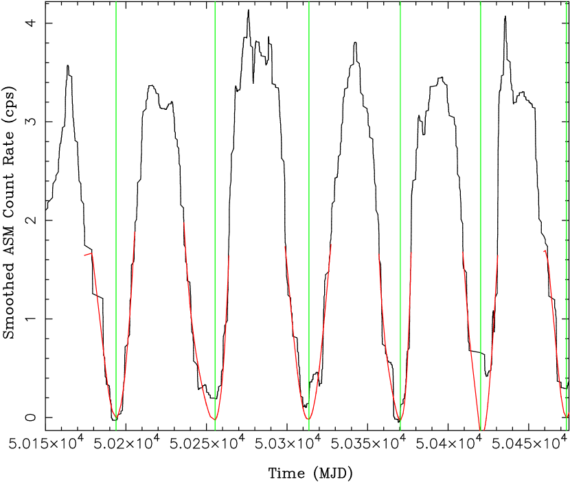
Figure 4.— SMCX-1 lightcurve between MJD 50150 and 50475, smoothed with a Gaussian filter. Fourth order polynomial fits in the minimum regions are superimposed. Minima of fits taken as the zero phase points for the super orbital period are denoted by vertical lines.

Using the lightcurve with the eclipse phases removed, the ASM lightcurve remains intrinsically noisy. For example, the peaks of each super-orbital cycle have a number of prominent dips (see Fig. 4), which appear to be akin to the “pre-eclipse dips” seen in the long term X-ray lightcurves of Her X-1 (Shakura et al. 1998; Stelzer et al. 1999; Klochkov et al. 2006). To further reduce the inherent noise in the ASM lightcurves of SMC X-1, we applied a simple Gaussian Smoothing to the unbinned ASM data via an FFT with a smoothing scale of 16 data bins ($\sim 2.5$ days on average). We defined low count regions by selecting regions of the lightcurve that were below a cutoff count value ($\leq$1.675 cps), and that were wide enough ($\geq$ 7 days) to assure that they were not residual noise fluctuations from the lightcurve. We then fit fourth order polynomials to each of the low count regions using the ISIS function array_fit, choosing a uniform weighting of the data points (see §2). We completed the definition of the super-orbital ephemeris by defining the minima of the polynomials in the low count regions as points of zero phase. This procedure is illustrated in Fig. 4, which shows a portion of the smoothed lightcurve with the polynomials and minima (zero-phase points) superimposed.

Table 2Super-Orbital Zero Phase Times and Lengths

Cycle Number	Start Time	Length	Cycle Number	Start Time	Length	Cycle Number	Start Time	Length
	(MJD)	(Days)		(MJD)	(Days)		(MJD)	(Days)
1	50193.8	61.6	25	51420.4	59.6	49	52824.5	48.6
2	50255.4	58.2	26	51479.9	69.7	50	52873.2	48.6
3	50313.6	56.5	27	51549.6	61.0	51	52921.8	47.8
4	50370.1	50.0	28	51610.6	63.0	52	52969.6	61.4
5	50420.1	53.2	29	51673.6	70.1	53	53031.0	52.5
6	50473.4	46.8	30	51743.7	57.1	54	53083.5	52.7
7	50520.2	52.0	31	51800.8	56.8	55	53136.2	54.0
8	50572.2	45.2	32	51857.5	48.8	56	53190.1	62.3
9	50617.4	47.3	33	51906.3	58.6	57	53252.4	59.6
10	50664.7	40.3	34	51964.9	54.8	58	53312.0	61.2
11	50705.0	43.0	35	52019.7	66.7	59	53373.2	46.5
12	50747.9	49.9	36	52086.4	48.8	60	53419.7	66.6
13	50797.9	39.6	37	52135.2	59.7	61	53486.3	62.7
14	50837.5	50.7	38	52194.9	50.6	62	53548.9	59.6
15	50888.2	44.3	39	52245.4	64.8	63	53608.5	62.2
16	50932.4	49.4	40	52310.3	62.3	64	53670.7	54.8
17	50981.9	45.2	41	52372.5	46.8	65	53725.5	54.6
18	51027.0	65.7	42	52419.4	56.6	66	53780.1	54.4
19	51092.7	52.6	43	52476.0	72.1	67	53834.5	44.4
20	51145.3	57.9	44	52548.1	50.5	68	53878.9	47.1
21	51203.2	58.5	45	52598.5	49.1	69	53926.0	47.8
22	51261.8	52.3	46	52647.6	44.1	70	53973.8	42.2
23	51314.0	58.5	47	52691.7	71.9	71	54016.0	39.0
24	51372.5	47.8	48	52763.6	60.9	$\cdots$	$\cdots$	$\cdots$

Note. — We estimate our methods for determining zero phase of the super-orbital cycles yields an uncertainty of about 2 days, which gives a corresponding uncertainty of $2\sqrt{2}$ days in the determination of the super-orbital cycle lengths.

Figure 5.— The time evolution of super-orbital cycle length. Error bars represent the uncertainty in cycle length due to the uncertainty in the determination of super-orbital zero phase times. The oscillatory structure superimposed on the long-term trend has previously been attributed to multiple warp modes in the disk (Clarkson et al. 2003).

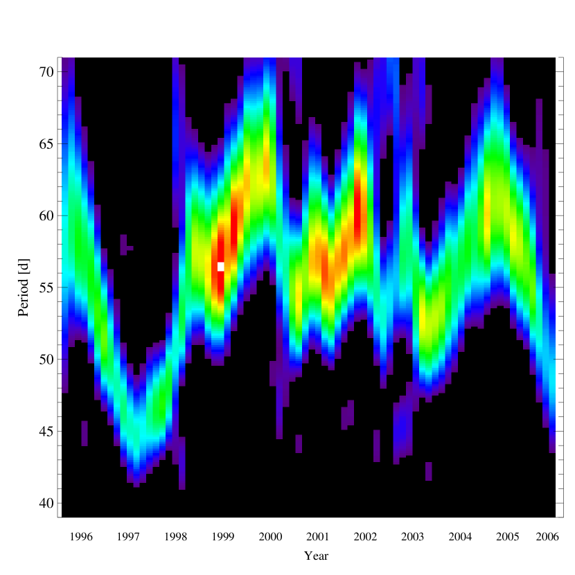
Figure 6.— Dynamical Lomb-Scargle periodogram for the entire ASM lightcurve of SMC X-1. The periodogram is calculated in 315 day intervals, slid 50 days each bin. (See Wilms et al. 2001.)

With the ephemeris defined as in Fig. 4, we were able to extract the start and stop time of each super-orbital cycle. We estimate, based upon multiple trials with variants of our zero-phase search routines (weighted averages, binned routines, to define the lightcurve, and several different functional forms to fit the minima) that our cycle start times have an accuracy of $\pm 2$ days. To search for possible patterns, we plotted the length of each super-orbital cycle versus the average date during that cycle. This plot is shown in Fig. 5. There appears to be a somewhat oscillatory trend, superimposed on a much longer time scale pattern. The longer term trends, especially the short (40–50 day) super-orbital cycles near the beginning of the ASM lightcurve, are likely what have been identified as multiple warp modes in the disk (i.e., Clarkson et al. 2003). Specifically, if we apply a sliding Lomb-Scargle periodogram to the ASM data (exactly as we have previously shown with ASM lightcurves of LMC X-3; Wilms et al. 2001), the rather ragged pattern of Fig. 5 appears more as a smooth evolution of super-orbital period, as shown in Fig. 6. Comparing to Fig. 5, however, we see that the smoothness of this trend is partly an artifact of the averaging process, and that a sliding Lomb-Scargle periodogram by itself is unrevealing for the fine detail of the evolution of this source.

We studied the distribution of these varying cycle lengths by creating a histogram of their values. The number of bins in the histogram was chosen because it produced the most easily seen pattern, but does not significantly change the results of the analysis. For example, doubling the number of bins does not change the shape of the distribution, except to add more noise to the overall trend. We found in this case that the distribution has a distinct double-peaked pattern, similar to other systems of this type. Specifically, such systems as Cyg X-2, LMC X-3, Cyg X-3 and Her X-1 show doubly peaked distributions for histograms of wait times between successive minima (Boyd & Smale 2004). It is possible that the SMC X-1 system is similarly oscillating (somewhat randomly) between two extreme periods. The profile of super-orbital cycle lengths is shown in Fig. 7.

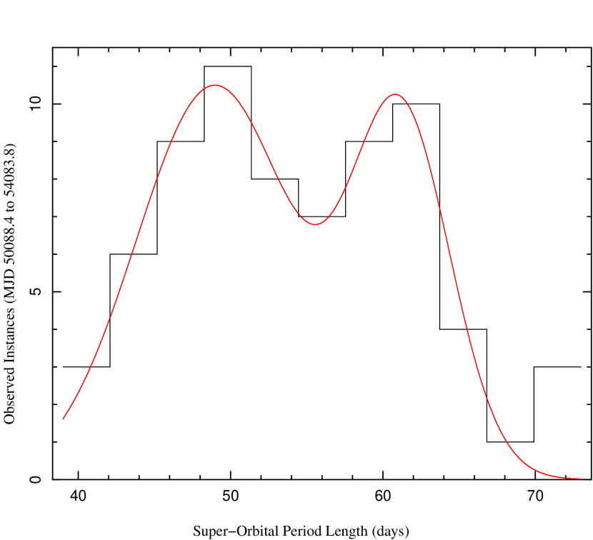
Figure 7.— Histogram distribution of super-orbital cycle lengths with bimodal (sum of two Gaussians) fit superimposed. The fit shown in this figure was used in the simulations described in §6.2.

Once we had defined the ephemeris, we attempted to find some correlation between the length of the super-orbital cycles and the X-ray flux from the system. Towards this end, for each super-orbital cycle we binned the rates into a histogram and attempted fits with several different functional forms; none of these were successful for all of the super-orbital cycles. This was due both to the large variance in the shapes of each super-orbital variation (including the aforementioned dips), as well as the lack of data for some portions of the lightcurve. Instead, we performed five point spline fits on each of the super-orbital cycles. From the spline fits we extracted the minimum, peak and mean flux during each super-orbital cycle and plotted each of those values against both the super-orbital cycle length, and the length minus its mean value of approximately 54.4 days. We were not able to find any correlations between super-orbital cycle length and flux with this method, nor by working on a coarser time scale, i.e., by averaging over five consecutive super-orbital cycles and searching for correlations between the same variables.

5. Folding on the Super-Orbital Period

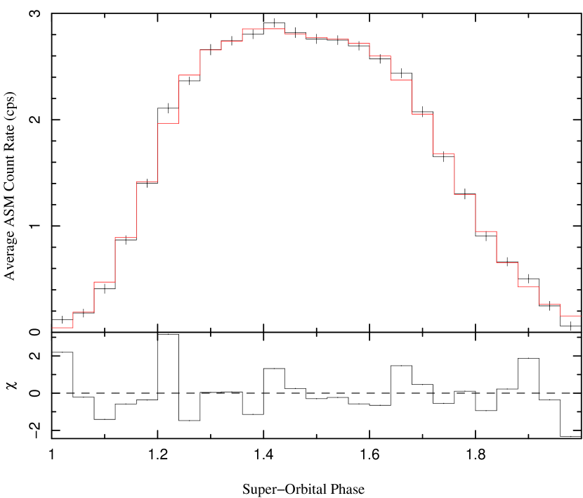
Figure 8.— Lightcurve Folded on super orbital period with fit of two superimposed Weibull functions.

With the super-orbital ephemeris defined, we were able to assign a super-orbital phase to each point on the lightcurve and proceed to fold the data over all super-orbital cycles. We chose to average the ASM lightcurve in 25 phase bins of the super-orbital cycles, and show the results in Fig. 8. It is interesting to note the asymmetry between the rise and fall of the curve, with the leading edge (super-orbital eclipse egress) exhibiting a much sharper rise than the falling edge’s decline. The best fit to this profile was obtained with the sum of two scaled Weibull functions (i.e., $\propto x^{\gamma}\exp[-(x/\beta)^{\alpha}]$; see Appendix B of Nowak et al. 1999 for historical references and description of the uses of this distribution function). We elected to use Weibull functions because their asymmetry can reasonably describe the asymmetry of the folded lightcurve. We used the sum of two curves as this matched the broadly peaked nature of the folded profile much better than did a single function. This was also suggested by the shape of the individual super-orbital cycle profiles, many of which were dramatically double peaked. Fit results are presented in Table 3.

Table 3Two Weibull Function Fits to Lightcurves Folded on Super-Orbital Cycle

ASM	$\chi^{2}_{red}$	Norm1	Peak1	$\alpha_{1}$	$\beta_{1}$	Norm2	Peak2	$\alpha_{2}$	$\beta_{2}$
Channel	(17 DoF)
1+2+3	1.95	$0.39^{+0.08}_{-0.01}$	$1.28^{+0.01}_{-0.00}$	$2.34^{+0.21}_{-0.02}$	$0.26^{+0.02}_{-0.00}$	$1.30^{+0.09}_{-0.10}$	$1.57^{+0.01}_{-0.00}$	$4.76^{+0.09}_{-0.55}$	$0.88^{+0.09}_{-0.10}$
1	2.41	$0.04^{+0.05}_{-0.02}$	$1.24^{+0.03}_{-0.03}$	$2.1^{+3.3}_{-0.8}$	$0.16^{+0.17}_{-0.07}$	$0.28^{+0.03}_{-0.07}$	$1.52^{+0.04}_{-0.03}$	$3.25^{+1.81}_{-0.03}$	$0.63^{+0.33}_{-0.23}$
2	2.07	$0.12^{+0.13}_{-0.03}$	$1.30^{+0.03}_{-0.01}$	$2.5^{+0.7}_{-0.4}$	$0.29^{+0.06}_{-0.05}$	$0.27^{+0.02}_{-0.03}$	$1.59^{+0.01}_{-0.00}$	$6.1^{+3.9}_{-1.9}$	$0.99^{+0.31}_{-0.48}$
3	1.61	$0.15^{+0.04}_{-0.01}$	$1.27^{+0.01}_{-0.01}$	$2.03^{+0.15}_{-0.05}$	$0.20^{+0.03}_{-0.01}$	$0.69^{+0.00}_{-0.40}$	$1.54^{+0.02}_{-0.01}$	$4.5^{+0.9}_{-0.5}$	$0.86^{+0.09}_{-0.09}$

Note. — Weibull functions had the form Norm${}_{1}(x-x_{0})\exp[-((x-x_{0})/\beta_{1})^{\alpha_{1}}]$, etc., where $x_{0}$ was determined by fixing the location of the function maximum to Peak₁. Error bars are 90% confidence levels.

Figure 9.— Color diagram for super-orbital profile. Emission is relatively monochromatic and dominated by hard X-rays. In lower intensity regions the emission is harder than in high intensity regions, which is in contrast to the eclipse emission in the average orbital profile.

As in our analysis of the orbital profile, using the data from the individual ASM energy channels we were able to create a super-orbital profile for each of the three energy channels. We fit each of these profiles with the same functional form used to fit the total profile. Fit results for the individual channels are also presented in Table 3. As expected from our analysis of the orbital profiles we once again found that the profile was dominated by high energy emission. Similar to our analysis of the average energy profile of the orbital variation, we created a color lightcurve for the super-orbital profile by plotting the color versus super-orbital phase, again using the definition of eq. (1). We present these results in Fig. 9. Once again we can see that the emission is fairly monochromatic, with two exceptions. Near phase 0.9 of the super-orbital period, there is weak evidence for a softening. More clear, however, is that near phase 0 of the super-orbital cycle (i.e., the low count rate region in which the neutron star is likely eclipsed by the disk) the emission appears to become harder, although the color values in this region have relatively large uncertainty. This is in marked contrast to the “bounceback” region of the orbital period fold, where the emission became softer. As in our color plot for the orbital profile, we have examined the same plot with a systematic shift upwards of 0.05 cps in all channels, however, in this case it does not significantly change the result.

6. Joint Orbital and Super-Orbital Profiles

6.1. Two Dimensional Phase Folds

To better understand the link between the orbital and super-orbital variations in SMC X-1, we created a two dimensional fold of the SMC X-1 lightcurve. Once we had defined an ephemeris for both the orbital and the super-orbital variations (as discussed in §3 and §4, respectively) we were able to assign every point on the lightcurve both an orbital and a super-orbital phase. We then created a grid of histogram bins with orbital phase on one axis and super-orbital phase on the other, and sorted the data points into that grid, averaging the intensity measurements in each bin. The result was the two dimensional histogram shown in Fig. 10. While we can observe the asymmetry noted in the super-orbital profile in this histogram, it does not contain sufficient statistics to give specific insight as to the evolution of orbital profile features at different super-orbital phases and vice versa. The choice of binning is made for maximum clarity. Unfortunately, current statistics are not sufficient such that finer binning would provide more information.

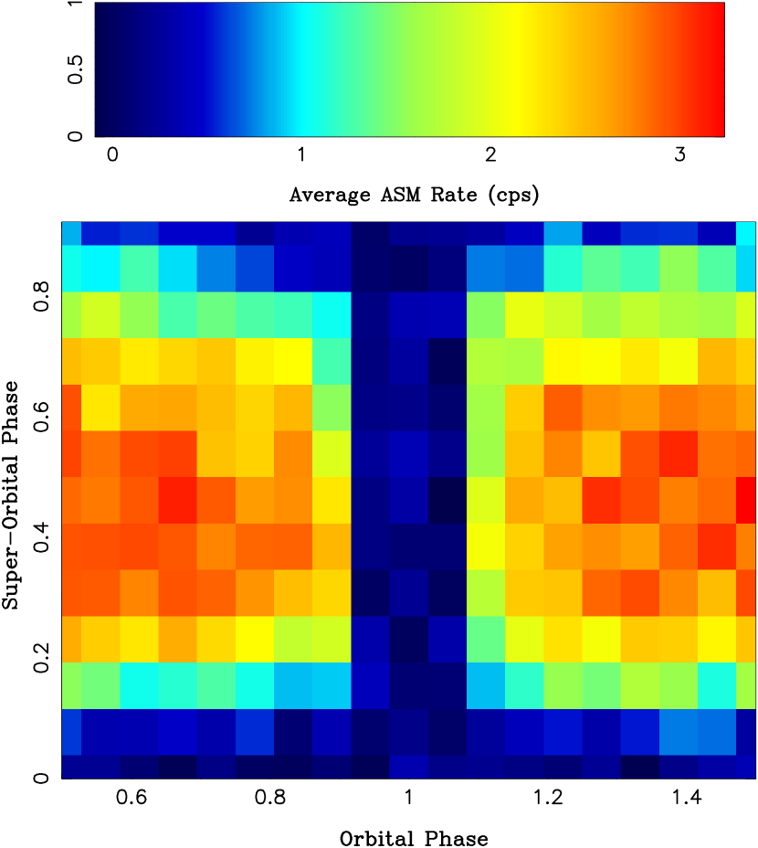
Figure 10.— Two dimensional folded lightcurve. Variation in orbital phase is plotted along the $x$-axis while super-orbital phase is plotted along the $y$-axis. The top panel shows the color scale.

To gain another visualization of the form of the orbital profile at different super-orbital phases, we also created several orbital profiles, each containing only points of the lightcurve in a small range of super-orbital phase, and plotted these profiles on a single set of axes. We present these orbital phase histograms in Fig. 11. Here again we find that we have insufficient statistics to demonstrate any definitive trends in the shape of the orbital profile dependent upon super-orbital phase. Further study of this system with better statistics (e.g., with a series of pointed X-ray observations) are likely necessary to witness any trends.

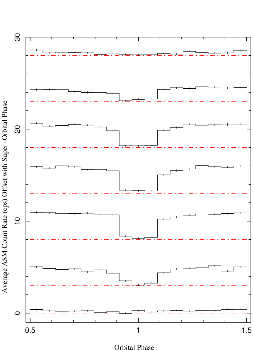
Figure 11.— Lightcurve folded on orbital period for specific ranges of super orbital phase, demonstrating the correlation between the two. Statistics are not good enough to enable identification and analysis of the bounceback feature in these folds.

6.2. Searching for Dependencies upon Orbital Period

In accordance with patterns seen in other sources, e.g., Her X-1 where the ‘turn on’ of the super-orbital cycle is tied to a half integer multiple of the orbital period (Staubert et al. 1983; Klochkov et al. 2006) or Cyg X-2 where the time between successive minima is an integer multiple of the orbital period (Boyd & Smale 2004), we searched for a correlation between the orbital period length and the super-orbital cycle lengths. We used a set of $\sim$3500 values between one quarter of the orbital period and one half of the longest observed super-orbital cycle to search for a value that divided most evenly into all of the super-orbital cycle lengths. For any given member of the set, we tested its relation to the super-orbital cycle lengths by dividing each of the 71 observed cycle lengths by that value, and summing the non-integer remainders of each of the 71 quotients. A value that fit relatively evenly into the set of super-orbital cycle lengths was one that exhibited a minimum value of the sum of non-integer parts. We found 16 values that exhibited minima in this formula, which we define as a point for which the sum of non-integer parts was $\leq$31. (The maximum value of the sum of the remainders was $\sim$43.6, while the mean of the sum was $\sim$36.2.) Of the 16 minima we found 7 that had some integer or quarter-integer relation to the orbital period, i.e., approximately 0.25, 0.5, 1, 2, 3, 5 and 6 times the orbital period length. The other 9 values that exhibited minima had no obvious relation to the orbital period length.

To test the significance of these observed values, we created a histogram of the sum of non-integer parts in order to study its distribution. The small value of this sum that we had obtained for 0.25, 0.5, 1, 2, 3, 5 and 6 times the orbital period length appeared rare, but not necessarily unusually so; therefore, we performed a Monte Carlo simulation to determine their significance. We first fit a bimodal (sum of two Gaussians) distribution to the super-orbital cycle length data shown in Fig. 7, from which we could randomly choose super-orbital period lengths. A single simulation consisted of randomly choosing 71 super-orbital cycle lengths from this distribution, and then performing the same analysis as done for the actual data. Specifically, the main goal was to create a histogram of the sum of non-integer parts from the quotients of each of the 3500 trial values with the chosen set of super-orbital cycle lengths. We performed $10^{6}$ such simulations and averaged all of the resulting histograms to obtain a theoretical distribution.

From this simulated distribution we could estimate the likelihood of obtaining the sums of non-integer remainders with values less than or equal to those that had been found for the quarter-integer and integer multiples of the orbital period. We found these probabilities to be $\approx$4.2%, 0.1%, 4.2%, 3.6%, 0.6%, 4.2% and 2.5% for the members of the set that were 0.25, 0.5, 1, 2, 3, 5 and 6 times the orbital period length, respectively. From these simulations we concluded that while these values appear to have interesting relations to the orbital period, and their corresponding sums of non-integer remainders are somewhat rare, they are not rare enough to point conclusively towards a relationship to the orbital period. Further study of this correlation – either via ASM observations with a longer baseline, or via pointed observations that can more accurately determine the start and stop times of each super-orbital period – may prove useful in determining if there truly is a relationship between the super-orbital cycle and orbital period lengths.

7. Summary

In our analysis of the ASM lightcurve of SMC X-1 we have observed several interesting features of both the orbital and super-orbital profiles. By using the ephemeris provided in Wojdowski et al. (1998), we were able to fold $\sim$11 years of data on orbital period to obtain an average orbital profile. The main results of this analysis are as follows.

• The lightcurve is characterized by complex modulation during the persistent emission (here modeled as a sinusoid, but which could possibly fit another model within the uncertainty), with a broad, asymmetric eclipse.

• We were able to witness a count rate bounceback phenomenon when averaging over large numbers of orbital cycles, which consists of a small rise and fall in counts during orbital mid-eclipse phases.

• The emission becomes somewhat softer during the eclipse/bounceback, while the persistent emission is fairly monochromatic.

Despite several pointed observations during orbital eclipse, in both low and high states of the super-orbital period, the bounceback has not been previously seen (Woo et al. 1995; Wojdowski et al. 1998). We did not have sufficient statistics to observe the dependence of this phenomenon on the super-orbital cycle, it is therefore possible that the bounceback is only present in certain super-orbital phases, or that its presence is only intermittent. Given the relatively few pointed observations of SMC X-1 during eclipse, it is possible prior pointed observations have simply not observed the state in which the bounceback is most prominent.

The softening during the eclipse might be akin to that seen in so-called Accretion Disk Corona (ADC) sources (White & Holt 1982). Such sources show broad, partial eclipses, with deeper eclipses in the hard X-ray (for example, see the lightcurves of X1822$-$371, Heinz & Nowak 2001). One model of these sources has a very spatially extended corona scattering X-ray from the central source into our line of sight; however, X-rays traveling through the atmosphere just above the midplane of the disk are preferentially absorbed in the soft X-rays (White & Holt 1982). Thus, the eclipse of the base of this extended corona is preferentially blocking harder X-rays, and leads to an overall softening of the spectrum. However, if such is occurring in SMC X-1, this does not explain the “bounceback” of the lightcurve. Perhaps additional scattering into our line of sight at orbital phase 0, from the atmosphere of the companion, rather than just an ADC, must also be invoked to explain the bounceback.

The super-orbital variation in SMC X-1 is not as easily dealt with as the orbital variation because of the complicated nature of the super-orbital ephemeris. The super-orbital cycle length is highly variable and Lomb-Scargle techniques alone are not sufficient to define its structure (Wen et al. 2006). In our analysis we were able to obtain a super-orbital ephemeris from the ASM data by modeling the locations of zero phase for each of 71 cycles. From that ephemeris we were able to extract an average super-orbital profile, as well as information about trends in the super-orbital cycle length. Our main results are as follows:

• In general we observe an asymmetry in the average super-orbital profile, most notable in a sharper rise in the low state egress than fall in the low state ingress.

• In contrast to the trend in the orbital profile, where we see softer emission during low count states, we find that emission appears to harden during low states in the super-orbital profile.

• We have found the lengths of the super-orbital cycles in SMC X-1 to be bimodally distributed, in agreement with Boyd & Smale (2004), and have also found suggestive, although not definitive, evidence that the variation in length is driven by some internal clock, the fundamental period of which is related to the orbital period as observed in Her X-1 and Cyg X-2. (Boyd & Smale 2004).

• In contrast to findings in analysis of Her X-1 (Still & Boyd 2004), we have been unable to find any correlation between the super-orbital cycle length, and X-ray flux.

• In contrast to Clarkson et al. (2003), who report a smooth evolution of the super-orbital cycle length, we observe sharp variations, often with large changes in length between adjacent super-orbital cycles.

This latter result is especially evident in observed super-orbital cycles 41 through 44 (MJD 52372.5 to 52598.5), in which the cycle duration rises from $\sim$47 days in cycle 41 to $\sim$72 days in cycle 43, and falls back to $\sim$50 days in cycle 44. Likewise between super-orbital cycles 46 through 49 (MJD 52647.6 to 52873.2) there is a rise from $\sim$44 days to $\sim$72 days in cycles 46 and 47, and a fall back to $\sim$49 days in cycle 49. Clarkson et al. (2003) also theorizes that the evolution of super-orbital cycle length is possibly sinusoidal. The lack of a regular, sinusoidal pattern in our data can easily be seen in Figs. 5 and 6.

In our spectral analysis of 71 super-orbital cycles we were able to observe a clear super-orbital profile in the first channel (1.2–3 keV), of an amplitude similar to that of the modulation in the second channel (3–5 keV; cf. Clarkson et al. 2003, who report little or no variation below 3 keV).

The most likely reason for the discrepancies between our analysis and that of Clarkson et al. (2003) is the extended length of the lightcurve we were able to analyze (about twice the length of that used in Clarkson et al. 2003) and our more precise definition of the edges of each individual period. The smoothing of super-orbital period length variation they observed is most likely at least partially an artifact of their use of a sliding Lomb-Scargle periodogram, and is similar to that we observed in Fig. 6.

The question then arises as to why SMC X-1 shows such extreme variations in its super-oribtal cycle length, while sources such as Her X-1 and LMC X-4 do not. Several tentative suggestions have been made based upon radiatively driven warp models. In such models, the driving force of the warp is the flux from the central source, which scales as $R^{-2}$, being absorbed and reradiated from the outer disk, whose intercepting area scales as $R^{2}$, thereby yielding a torque that increases linearly with distance. Disks can therefore become unstable to radiative driving of a warp if they are large enough (and the accretion efficiency is high enough; Pringle 1996), which is a function of the system’s orbital period and secondary to primary mass ratio. Numerical simulations (Wijers & Pringle 1999) and analytic estimates (Ogilvie & Dubus 2001) indicate that the Her X-1 system is just large enough to have a stable warp. The analytic models, however, also indicate that the, rather complex in terms of their eigenvalue behavior, underlying equations only admit stable warp solutions for a finite range of disk sizes (Ogilvie & Dubus 2001). Estimates are that SMC X-1 may be near the upper limit of system sizes that are unstable to warping, and therefore may be more likely to exhibit chaotic warp modes. Our results are certainly consistent with that expectation.

Within the framework of a radiatively driven warp, the existence and stability of the warp modes are also dependent upon the radius at which matter is injected into the disk (Wijers & Pringle 1999; Ogilvie & Dubus 2001). Being more heavily wind-fed, this may be another way in which SMC X-1 differs from Her X-1. Perhaps variations in the wind speed of the SMC X-1 secondary, leading to variations of the disk circularization radius (equated with the mass injection radius in the majority of theoretical models) may account for the varying cycle lengths. An ASM study like the one presented here, coupled with spectroscopic observations of the secondary’s wind, may be an avenue for exploring such a possibility.

The above speculations, however, do not account for the possibility of a fundamental “underlying clock” for the SMC X-1 super-orbital cycles. In their analysis of several X-ray binary systems Boyd & Smale (2004) find many systems for which the super-orbital excursion lengths are random integer multiples of some fundamental period, (Cyg X-2, LMC X-3 and Cyg X-3). They also find, when plotting the lightcurves of the systems in $X,\dot{X}$ phase space, that each of these sources demonstrates circulation in the phase space about two rotation centers, creating a bimodal distribution in the length of super-orbital variations. SMC X-1 shows similar characteristics.

Wijers & Pringle (1999) speculated that for sufficiently large amplitude warps, the effective mass injection radius (i.e., where the incoming accretion flow interacts with and circularizes into the inclined disk) could greatly fluctuate from one super-orbital cycle to the next, causing fluctuations in cycle duration that become tied to the orbital period. An avenue for exploring this possibility may be to model individual cycles of the ASM lightcurve, to see if one can discern a changing warp amplitude with each cycle. The fact, however, that we did not find a dependence of cycle duration upon mean, minimum, or peak ASM flux, may argue against this possibility.

To summarize, using the ASM lightcurve, we have defined a super-orbital ephemeris for SMC X-1 for 1995-2006. It will now be possible to put pointed observations during this period in the context of both the orbital ephemeris from Wojdowski et al. (1998) and the super-orbital ephemeris from this work. We have exploited the spectral information from the three channels of the ASM as much as possible and extracted information from the spectrum in both the orbital and super-orbital profiles, to guide both further observations, as well as theories, e.g., of disk warping, which currently do not describe behavior as complex as that seen here in SMC X-1. It is also now necessary to perform multiple pointed observations in order to observe a variety of super-orbital and orbital phase combinations and gather better statistics than provided by the data analyzed in this study. It might then be possible to analyze the super-orbital evolution of orbital profile features, including the bounceback. With pointed observations we might also be able to better analyze the super-orbital ingress and egress and the spectral variation in the emission, to obtain more insight into the structure of the HMXB SMC X-1 and other similar systems.

References

- Boyd & Smale (2004) Boyd, P. T. & Smale, A. P. 2004, ApJ, 612, 1006
- Caproni et al. (2006) Caproni, A., Livio, M., Abraham, Z., & Mosquera Cuesta, H. J. 2006, ApJ, 653, 112
- Clarkson et al. (2003) Clarkson, W. I., Charles, P. A., Coe, M. J., Laycock, S., Tout, M. D., & Wilson, C. A. 2003, MNRAS, 339, 447
- Gruber & Rothschild (1984) Gruber, D. E. & Rothschild, R. E. 1984, ApJ, 283, 546
- Heinz & Nowak (2001) Heinz, S. & Nowak, M. A. 2001, MNRAS, 320, 249
- Houck & Denicola (2000) Houck, J. C. & Denicola, L. A. 2000, in ASP Conf. Ser. 216: Astronomical Data Analysis Software and Systems IX, Vol. 9, 591
- Katz (1973) Katz, J. I. 1973, Nature, 246, 87
- Klochkov et al. (2006) Klochkov, D., Shakura, N., Postnov, K., Staubert, R., Wilms, J., & Ketsaris, N. 2006, PAZH, in press
- Leong et al. (1971) Leong, C., Kellogg, E., Gursky, H., Tananbaum, H., & Giacconi, R. 1971, ApJ, 170, L67
- Levine et al. (1996) Levine, A. M., Bradt, H., Cui, W., Jernigan, J. G., Morgan, E. H., Remillard, R., Shirey, R. E., & Smith, D. A. 1996, ApJ, 469, L33
- Liller (1973) Liller, W. 1973, ApJ, 184, L37
- Lomb (1976) Lomb, N. R. 1976, Ap&SS, 39, 447
- Lucke et al. (1976) Lucke, R., Yentis, D., Friedman, H., Fritz, G., & Shulman, S. 1976, ApJ, 206, L25
- Maloney et al. (1996) Maloney, P. R., Begelman, M. C., & Pringle, J. E. 1996, ApJ, 472, 582
- Nowak et al. (1999) Nowak, M. A., Wilms, J., Vaughan, B. A., Dove, J., & Begelman, M. C. 1999, ApJ, 515, 726
- Ogilvie & Dubus (2001) Ogilvie, G. I. & Dubus, G. 2001, MNRAS, 320, 485
- Petterson (1977) Petterson, J. A. 1977, ApJ, 214, 550
- Pringle (1996) Pringle, J. E. 1996, MNRAS, 281, 357
- Scargle (1982) Scargle, J. D. 1982, ApJ, 263, 835
- Schreier et al. (1972) Schreier, E., Giacconi, R., Gursky, H., Kellogg, E., & Tananbaum, H. 1972, ApJ, 178, L71
- Shakura et al. (1998) Shakura, N. I., Ketsaris, N. A., Prokhorov, M. E., & Postnov, K. A. 1998, MNRAS, 300, 992
- Staubert et al. (1983) Staubert, R., Bezler, M., & Kendziorra, E. 1983, A&A, 117, 215
- Stelzer et al. (1999) Stelzer, B., Wilms, J., Staubert, R., Gruber, D., & Rothschild, R. 1999, A&A, 342, 736
- Still & Boyd (2004) Still, M. & Boyd, P. 2004, ApJ, 606, L135
- Tananbaum et al. (1972) Tananbaum, H., Gursky, H., Kellogg, E. M., Levinson, R., Schreier, E., & Giaconi, R. 1972, ApJ, 174, L143
- Webster et al. (1972) Webster, B. L., Martin, W. L., Feast, M. W., & Andrews, P. J. 1972, Nature, 240, 183
- Wen et al. (2006) Wen, L., Levine, A. M., Corbet, R. H. D., & Bradt, H. V. 2006, ApJS, 163, 372
- White & Holt (1982) White, N. E. & Holt, S. S. 1982, ApJ, 257, 318
- Wijers & Pringle (1999) Wijers, R. A. M. J. & Pringle, J. E. 1999, MNRAS, 308, 207
- Wilms et al. (2001) Wilms, J., Nowak, M. A., Pottschmidt, K., Heindl, W. A., Dove, J. B., & Begelman, M. C. 2001, MNRAS, 320, 316
- Wojdowski et al. (1998) Wojdowski, P., Clark, G. W., Levine, A. M., Woo, J. W., & Zhang, S. N. 1998, ApJ, 502, 253
- Woo et al. (1995) Woo, J. W., Clark, G. W., Blondin, J. M., Kallman, T. R., & Nagase, F. 1995, ApJ, 445, 896