Survey Requirements for Accurate and Precise Photometric Redshifts for Type Ia Supernovae

Abstract

In this paper we advance the simple analytic photometric redshift estimator for Type Ia supernovae (SNe Ia) proposed by Wang (2007), and use it to study simulated SN Ia data. We find that better than 0.5% accuracy in $z_{\rm phot}$ (with $\sigma[(z_{\rm phot}-z_{\rm spec})/(1+z_{\rm spec})]<0.005$) is possible for SNe Ia with well sampled lightcurves in three observed passbands ($riz$) with a signal-to-noise ratio of 25 at peak brightness, if the extinction by dust is negligible. The corresponding bias in $z_{\rm phot}$ (the mean of $z_{\rm phot}-z_{\rm spec}$) is $5.4\times 10^{-4}$. If dust extinction is taken into consideration in the $riz$ observer-frame lightcurves, the accuracy in $z_{\rm phot}$ deteriorates to 4.4%, with a bias in $z_{\rm phot}$ of $8.0\times 10^{-3}$. Adding the $g$ band lightcurve improves the accuracy in $z_{\rm phot}$ to 2.5%, and reduces the bias in $z_{\rm phot}$ to $-1.5\times 10^{-3}$. Our results have significant implications for the design of future photometric surveys of SNe Ia from both ground and space telescopes. Accurate and precise photometric redshifts boost the cosmological utility of such surveys.

1 Introduction

The discovery of cosmic acceleration (Riess et al., 1998; Perlmutter et al., 1999) was made using Type Ia supernovae (SNe Ia) as cosmological standard candles (Phillips, 1993; Riess, Press, & Kirshner, 1995). The unknown reason for the observed cosmic acceleration has been dubbed “dark energy”. Obtaining the spectroscopic redshifts of SNe Ia is the most costly aspect of supernova surveys. Large photometric surveys of SNe Ia have been planned to help illuminate the nature of dark energy. Obtaining accurate and precise photometric redshifts (photo-$z$’s) will be key in maximizing the cosmological utility of such surveys (Huterer et al., 2004).

In this paper, we advance the simple analytic photometric redshift estimator for Type Ia supernovae (SNe Ia) proposed by Wang (2007), and use it to study simulated SN Ia data. In order to derive unbiased and accurate photo-$z$’s, it will be important to develop a variety of different techniques to cross-check sensitivities to various systematic uncertainties and correctly calculating the covariance between distance modulus and photo-$z$ when fitting for cosmological parameters.

We present our method in Sec. 2 and the results in Sec. 3. We discuss and summarize in Sec. 4.

2 The Method

2.1 The analytic photo-$z$ estimator

The analytic photo-$z$ estimator for SNe Ia proposed by Wang (2007) is empirical, model independent (no templates used), and uses observables that reflect the properties of SNe Ia as calibrated standard candles. It was developed using the SN Ia data released by the Supernova Legacy Survey (Astier et al., 2006).

This estimator uses the fluxes in $griz$ (or $riz$) at the epoch of $i$ maximum flux to make an effective K-correction to the $i$ flux. The first estimate of redshift is given by

$$z_{\rm phot}^{0}=c_{1}+c_{2}g_{f}+c_{3}r_{f}+c_{4}i_{f}+c_{5}z_{f}+c_{6}i_{f}^{2}+c_{7}i_{f}^{3}$$ (1)

where $g_{f}=2.5\log(f_{g})$, $r_{f}=2.5\log(f_{r})$, $i_{f}=2.5\log(f_{i})$, and $z_{f}=2.5\log(f_{z})$, and $f_{g}$, $f_{r}$, $f_{i}$, $f_{z}$ are fluxes in counts, normalized to some fiducial zeropoint, in $griz$ at the epoch of $i$ maximum flux.

Next, it calibrates each SN Ia in its estimated rest-frame using

$$\Delta i_{15}=2.5\log(f_{i}^{15d}/f_{i}),$$ (2)

where $f_{i}^{15d}$ is the $i$ band flux at 15 days after the $i$ flux maximum in the estimated rest-frame, corresponding to the epoch of $\Delta t^{15d}=15(1+z_{\rm phot}^{0})$ days after the epoch of $i$ flux maximum.

The final estimate for the photometric redshift is given by

$$z_{\rm phot}=\sum_{i=1}^{8}c_{i}\,p_{i},$$ (3)

where the data vector ${\mbox{\bf p}}=\{1,g_{f},r_{f},i_{f},z_{f},i_{f}^{2},i_{f}^{3},\Delta i_{15}\}$. The coefficients $c_{i}$ (i=1,2,…,8) are found by using a training set of SNe Ia with $griz$ (or $riz$, for which $c_{2}=0$) lightcurves and measured spectroscopic redshifts. We use the jackknife technique (Lupton, 1993) to estimate the mean and the covariance matrix of $c_{i}$ (see Sec. 3).

2.2 Simulation of data

SN Ia lightcurves for training and testing were simulated using the templates and various routines from MLCS2k2 (Jha et al., 2007). We created two sets of $griz$ lightcurves using the MLCS2k2 “final” templates at random redshifts in the range $0.001\leq z\leq 1$ with S/N=25 at peak and $\Delta$, the parameter that MLCS2k2 uses to describe the variation in the SN Ia lightcurves, fixed to $0$. The luminosity distance $\mu$, is calculated from the redshift assuming a flat cosmology with $\Omega_{M}=0.3$, $h=0.65$ and $w=-1$. The particular choice of cosmology will not affect the photo-$z$ estimator as long as the training and testing lightcurves are consistent with each other.

The first training set consists of 100 lightcurves and was simulated with no host extinction. The corresponding blind test set contains 1000 lightcurves similar to those in the training set.

The second training set consists of 200 lightcurves, and has $A_{V}$ drawn at random from the “default” distribution, an exponential decay with argument $0.46$ mag and zero for $A_{V}<0$ mag, following Jha et al. (2007). The particular form of this exponential tail is derived from the observation (Lira, 1995) that SNe Ia have a common color at $\sim 40$ days past peak. We assume the extinction law to be $R_{V}=3.1$. We used a larger training set of 200 simulated lightcurves for training to compensate for the larger variation in the data caused by including extinction. The corresponding blind test set contains 1000 lightcurves similar to those in the training set.

The actual training sets and blind test sets used are slightly smaller than described above, because only SNe Ia with $riz$ lightcurves, i.e. $z\leq 0.95$, are used in this paper. We use the training sets to derive the photo-$z$ coefficients and their covariance matrix (see Eq. 3 and Sec. 3), and the blind test sets to evaluate the performance of the photo-$z$ estimator.

3 Results

We use a slightly modified version of the jackknife technique (Lupton, 1993) to estimate the mean and the covariance matrix of $c_{i}$. From the training set containing $N$ SNe Ia, we extract $N$ subsamples each containing $N-1$ SNe Ia by omitting one SN Ia. The coefficients $c_{i}^{(s)}$ (i=1,2,…,8) for the $s$-th subsample are found by a maximum likelihood analysis matching the predictions of Eq. 3 with the spectroscopic redshifts.

The mean of the coefficients $c_{i}$ (i=1,2,…,8) are given by

$$\langle c_{i}\rangle=\frac{1}{N}\sum_{s=1}^{N}c_{i}^{(s)}.$$ (4)

Note that this is related to the usual “bias-corrected jackknife estimate” for $c_{i}$, $c_{i}^{J}$, as follows:

$$c_{i}^{J}\equiv c_{i}^{N}+(N-1)\left(c_{i}^{N}-\langle c_{i}\rangle\right),$$ (5)

where $c_{i}^{N}$ are estimated from the entire training set (with $N$ SNe Ia). We found that for small training sets (with $N<20$) that include SNe Ia at $z\sim 0$, $c_{i}^{J}$ give biased estimates of $c_{i}$ by giving too much weight to the SN Ia with the smallest redshift. For training sets not including nearby SNe Ia, $\langle c_{i}\rangle$ and $c_{i}^{J}$ are approximately equal. We have chosen to use $\langle c_{i}\rangle$ from Eq. 4 as the mean estimates for $c_{i}$ to avoid biased $z_{\rm phot}$ for SNe Ia at $z$ close to zero.

The covariance matrix of $c_{i}$ (i=1,2,…,8) are given by

$${\rm Cov}(c_{i},c_{j})=\frac{N-1}{N}\sum_{s=1}^{N}\left(c_{i}^{(s)}-\langle c_{i}\rangle\right)\,\left(c_{j}^{(s)}-\langle c_{j}\rangle\right)$$ (6)

Since $z_{\rm phot}=\sum c_{i}p_{i}$, $\Delta z_{\rm phot}=\sum p_{i}\Delta c_{i}$, since the uncertainty in $z_{\rm phot}$ is dominated by the uncertainty in $c_{i}$. Therefore estimated error in $z_{\rm phot}$ is

$${\rm d}z_{\rm phot}=\left\{\sum_{i=1}^{8}\sum_{j=1}^{8}[p_{i}]\,{\rm Cov}(c_{i},c_{j})[p_{j}]\right\}^{1/2},$$ (7)

where ${p_{i}}$ and ${p_{j}}$ (i,j=1,2,…8) are the $i$-th and $j$-th components of the data vector ${\mbox{\bf p}}=\{1,g_{f},r_{f},i_{f},z_{f},i_{f}^{2},i_{f}^{3},\Delta i_{15}\}$.

In applying the photo-$z$ estimator to simulated data, we find that applying it to the entire data set leads to substructure in the estimated $z_{\rm phot}$. Therefore, we divide the training set into three $i$ maximum flux ranges (corresponding to three roughly equal redshift intervals), and applying the photo-$z$ estimator to each flux range.

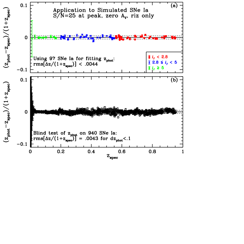
Fig. 1 shows the resultant performance of the photo-$z$ estimator for simulated SN Ia lightcurves in $riz$, with S/N=25 at peak brightness, and zero extinction due to dust. The top panel shows the training set of 97 SNe Ia, with different point types and color denoting different flux ranges. The $c_{i}$’s derived from the training set are used to predict $z_{\rm phot}$ for a blind-test set of 940 SNe Ia (divided into the same flux ranges as the training set), with the results shown in the bottom panel of Fig. 1.

The results for the blind-test set closely mimic that of the training set. Since the data are very sparse at $z<0.02$ due to the small size of the training set, the estimated uncertainty on $z_{\rm phot}$, d$z_{\rm phot}$, becomes large for nearby SNe Ia. Since d$z_{\rm phot}$ is a reliable indicator of the accuracy of $z_{\rm phot}$, we can use d$z_{\rm phot}$ to exclude the SNe Ia with estimated $z_{\rm phot}$ not suitable for inclusion in the cosmological data set.

We find that d$z_{\rm phot}<0.1$ only excludes 9 out of the 940 SNe Ia in the blind-test set, all at $z<0.02$. For the culled blind-test set of 931 SNe Ia (d$z_{\rm phot}<0.1$), $\sigma[(z_{\rm phot}-z_{\rm spec})/(1+z_{\rm spec})]=0.0043$. The corresponding bias in $z_{\rm phot}$ (the mean of $z_{\rm phot}-z_{\rm spec}$) is $5.4\times 10^{-4}$ overall and is $[0.48,0.79,1.5,-0.81]\times 10^{-3}$ in the 4 redshift bins bounded by $[0,0.25,0.5,0.75,1]$.

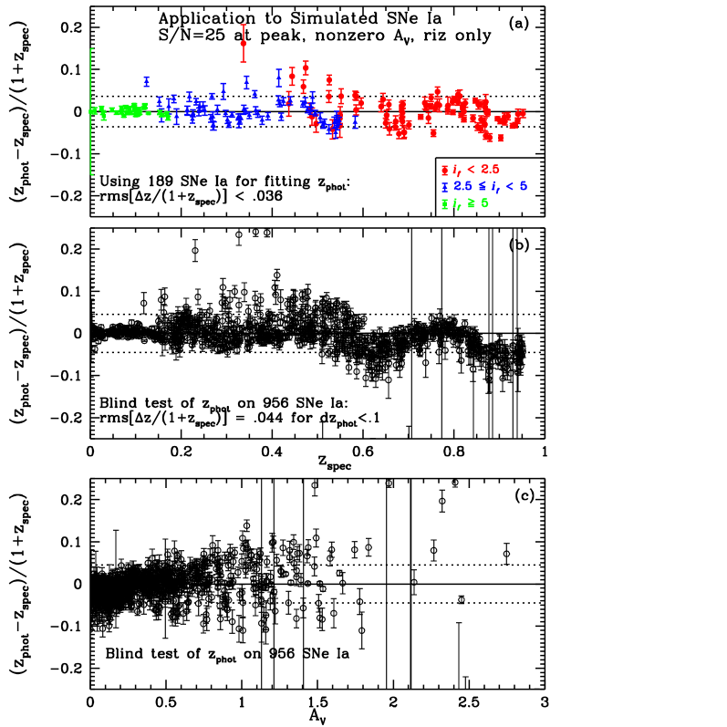
Fig. 2 shows the performance of the photo-$z$ estimator for simulated SN Ia lightcurves in $riz$, with S/N=25 at peak brightness, and extinction due to dust parameterized by $A_{V}$. Again, we cull the blind-test set by requiring that d$z_{\rm phot}<0.1$; this excludes 16 out of the 956 SNe Ia, most of which are highly extinguished or have very low $z$. The inclusion of dust extinction leads to a deteriorated accuracy in $z_{\rm phot}$ of 4.4%. The corresponding bias in $z_{\rm phot}$ is $8.0\times 10^{-3}$ overall and is $[-9.3,-22.,25.,53.]\times 10^{-3}$ in the 4 redshift bins bounded by $[0,0.25,0.5,0.75,1]$.

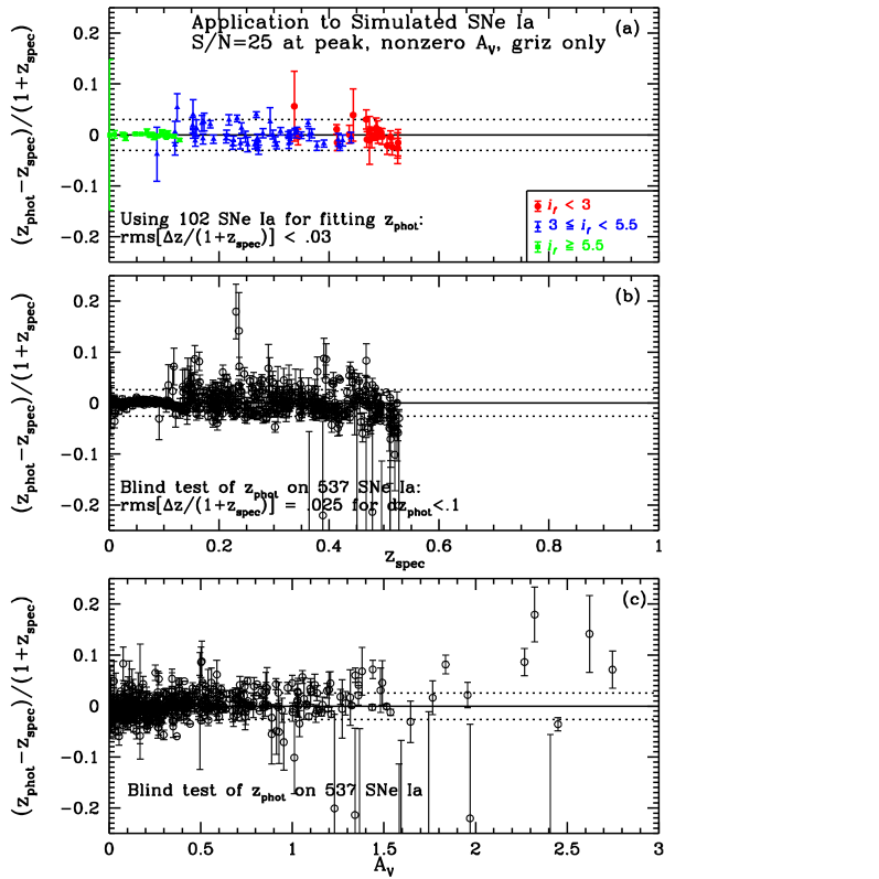
Fig. 3 is similar to Fig. 2, but only the subsets of data (both the training set and the blind-test set) with $g$ band lightcurves are included. Note that the $i$ maximum flux ranges in Fig. 3 are similar to Fig. 2, but slightly adjusted to make sure that the sub sample with the smallest fluxes contains enough SNe Ia. The SNe Ia at $z>0.54$ in our simulated data set do not have $g$ band lightcurves, as these require rest-frame lightcurve templates bluer than $u$ band, which are not yet readily available.

Imposing d$z_{\rm phot}<0.1$ excludes 12 out of the 537 SNe Ia, most of which are highly extinguished or have very low $z$. Adding the $g$ band lightcurves improve the accuracy in $z_{\rm phot}$ to 2.5%. The corresponding bias in $z_{\rm phot}$ is reduced to $-1.5\times 10^{-3}$ overall and is $[-6.0,3.2]\times 10^{-3}$ in the 2 redshift bins bounded by $[0,0.266,0.532]$.

4 Discussion and Summary

Accurate and precise photo-$z$’s will be critical for enabling cosmology with future large SNe Ia photometric surveys (Huterer et al., 2004). In this paper, we have advanced the empirical and analytic photo-$z$ estimator proposed by Wang (2007) and used it to study simulated data in order to derive the survey requirements for accurate and precise photo-$z$’s for SNe Ia from large photometric surveys. Future work will explore the critically-important question of the degree of covariance between the redshift determined using this method and the distance modulus determined by using a luminosity distance fitter since it is these two parameters that form the basis for the cosmological measurements with SNe Ia.

We apply the photo-$z$ estimator to $riz$ data divided into $i$ maximum flux ranges that roughly correspond to equal redshift intervals (see Fig. 1 and Fig. 2). We use d$z_{\rm phot}<0.1$ as a quality measurement to cull the blind-test set. This cut only excludes $<2$% of the SNe Ia, most of which are highly extinguished or are at very low $z$. To derive accurate cosmological constraints, it is optimal to combine the very large set of SNe Ia with well estimated photo-$z$’s with a small spectroscopic sample of SNe Ia at very low $z$ expected from ongoing nearby surveys (Huterer et al., 2004). SNe Ia at $z<0.025$ are currently excluded from SN Ia cosmological analyses even for spectroscopic data, because peculiar velocities due to cosmic large scale structure modifies the Hubble diagram of nearby standard candles (Wang, Spergel, & Turner, 1998), and have the largest impact on the nearest SNe Ia (see, e.g., Zehavi et al. (1998); Cooray & Caldwell (2006); Hui & Greene (2006); Conley et al. (2007)).

We find that determining $z_{\rm phot}$’s with better than 0.5% accuracy (RMS[$\Delta z_{\rm phot}/(1+z_{\rm spec})]$ = 0.0043%) and negligible bias ($\langle z_{\rm phot}-z_{\rm spec}\rangle=5.4\times 10^{-4}$) is possible if dust extinction can be neglected, for SNe Ia with well sampled lightcurves in $riz$ and S/N=25 at peak brightness. The inclusion of dust extinction leads to a drastic deterioration of the accuracy of $z_{\rm phot}$ (RMS[$\Delta z_{\rm phot}/(1+z_{\rm spec})]$ = 4.4%, and $\langle z_{\rm phot}-z_{\rm spec}\rangle=8.0\times 10^{-3}$). Adding the $g$ band lightcurve significantly improves the accuracy and precision of $z_{\rm phot}$ with RMS[$\Delta z_{\rm phot}/(1+z_{\rm spec})$] = 2.5%, and $\langle z_{\rm phot}-z_{\rm spec}\rangle=-1.5\times 10^{-3}$.

Future supernova surveys can easily obtain the multi-band photometry of a huge number of supernovae (Wang, 2000; Wang et al., 2004; Phillips et al., 2006). We only considered $griz$ photometry in this paper, due to the limitation of currently available SN Ia lightcurve templates. The addition of photometry at longer wavelengths should provide more dramatic improvement on the accuracy and precision of $z_{\rm phot}$ since extinction decreases with wavelength, and SNe Ia are better standard candles in the near IR (Krisciunas, Phillips, & Suntzeff, 2004). In future work, we will study simulated SN Ia data over the entire wavelength range of relevance to future observations, and examine the impact of realistic survey and observational parameters on the precision and accuracy of our photo-$z$ estimator.

Our results are encouraging for the prospect of using photometric surveys to constrain cosmology, such as those planned for the Advanced Liquid-mirror Probe for Astrophysics, Cosmology and Asteroids (ALPACA); Pan-STARRS; the Dark Energy Survey (DES); and the Large Synoptic Survey Telescope (LSST).

Acknowledgments We thank the Aspen Center for Physics for hospitality where part of the work was done. We are grateful to Alex Kim for useful discussions. YW is supported in part by NSF CAREER grant AST-0094335. MWV is supported in part by NSF AST-057475.

Figure 1: The analytic photo-$z$ estimator applied to simulated SN Ia lightcurves in $riz$, with S/N=25 at peak brightness, and zero extinction due to dust.

Figure 2: The analytic photo-$z$ estimator applied to simulated SN Ia lightcurves in $riz$, with S/N=25 at peak brightness, and dust extinction parameterized by $A_{V}$. Dust extinction leads to deterioration in the accuracy of $z_{\rm phot}$. The y-axis range is the same as in Fig. 3.

Figure 3: The analytic photo-$z$ estimator applied to simulated SN Ia lightcurves in $griz$, with S/N=25 at peak brightness, and dust extinction parameterized by $A_{V}$. Adding the $g$ band lightcurves improves the accuracy of $z_{\rm phot}$. The y-axis range is the same as in Fig. 2.

References

- Astier et al. (2006) Astier, P., et al. 2006, A & A 447, 31-48 (2006)
- Conley et al. (2007) Conley, A., et al. 2007, arXiv:0705.0367v2, ApJL, in press
- Cooray & Caldwell (2006) Cooray, A.; Caldwell, R.R. 2006, Phys.Rev.D73, 103002
- Guy et al. (2007) Guy, J., et. al. 2007, A & A, in press, arXiv:astro-ph/0701828v1
- Hui & Greene (2006) Hui, L.; & Greene, P.B. 2006, Phys. Rev. D73, 123526
- Huterer et al. (2004) Huterer, D.; Kim, A.; Krauss, L.M.; Broderick, T. 2004, ApJ, 615, 595
- Jha et al. (2007) Jha, S.; Reiss, A. G.; Kirshner, R. P. 2007, ApJ, 659, 122 arXiv:astro-ph/0612666
- Krisciunas, Phillips, & Suntzeff (2004) Krisciunas, K.; Phillips, M.M.; Suntzeff, N.B. 2004, ApJ, 602, L81
- Lira (1995) Lira, P. 1995, Master’s thesis, University of Chile
- Lupton (1993) Lupton, R., 1993, “Statistics in Theory and Practice”, Princeton University Press
- Perlmutter et al. (1999) Perlmutter, S. et al., 1999, ApJ, 517, 565
- Phillips (1993) Phillips, M.M. 1993, ApJ, 413, L105
- Phillips et al. (2006) Phillips, M. M.; Garnavich, P.; Wang, Y. et al. 2006, Proc. of SPIE, Volume 6265, 626529, arXiv:astro-ph/0606691v1
- Riess, Press, & Kirshner (1995) Riess, A.G., Press, W.H., and Kirshner, R.P. 1995, ApJ, 438, L17
- Riess et al. (1998) Riess, A. G, et al., 1998, Astron. J., 116, 1009
- Wang (2000) Wang, Y. 2000, ApJ 531, 676
- Wang, Bahcall, & Turner (1998) Wang, Y.; Bahcall, N.; Turner, E. L., 1998, AJ, 116, 2081
- Wang, Spergel, & Turner (1998) Wang, Y.; Spergel, D.N.; & Turner, E.L. 1998, ApJ, 498, 1
- Wang et al. (2004) Wang, Y., et al. 2004 (the JEDI Collaboration), BAAS, v36, n5, 1560. See also http://jedi.nhn.ou.edu/.
- Wang (2007) Wang, Y. 2007, ApJ, 654, L123
- Zehavi et al. (1998) Zehavi, I.; Riess, A.G.; Kirshner, R.P.; & Dekel, A. 1998, ApJ, 503, 483