Goal-oriented Atomistic-Continuum Adaptivity for the Quasicontinuum Approximation

Abstract.

We give a goal-oriented a posteriori error estimator for the atomistic-continuum modeling error in the quasicontinuum method, and we use this estimator to design an adaptive algorithm to compute a quantity of interest to a given tolerance by using a nearly minimal number of atomistic degrees of freedom. We present computational results that demonstrate the effectiveness of our algorithm for a periodic array of dislocations described by a Frenkel-Kontorova type model.

1. Introduction

Multiscale methods offer the potential to solve complex problems by utilizing a fine-scale model only in regions that require increased accuracy. However, it is usually not known a priori which region requires the increased accuracy, and an adaptive algorithm is needed to compute a given quantity of interest to a given tolerance with nearly optimal computational efficiency.

The quasicontinuum (QC) method [9, 10, 11, 4] is a multiscale computational method for crystals that retains sufficient accuracy of the atomistic model by utilizing a strain energy density obtained from the atomistic model by the Cauchy-Born rule in regions where the deformation is nearly uniform. The atomistic model is needed to accurately model the material behavior in regions of highly non-uniform deformations around defects such as dislocations and cracks.

The approximation error within the quasicontinuum method can be decomposed into the modeling error which occurs when replacing the atomistic model by a continuum model, and the coarsening error which arises from reducing the number of degrees of freedom within the continuum region. This paper purely focuses on the estimation of the modeling error. The optimal strategy to determine the mesh size in the continuum region will be studied in a forthcoming paper.

The development of goal-oriented error estimators for mesh coarsening in the quasicontinuum method has been given in [7, 6], and goal-oriented error estimators for atomistic-continuum modeling have recently been given in [2]. In all these works, the error is measured in terms of a user-definable quantity of interest instead of a global norm. Goal-oriented error estimation in general is based on duality techniques and has already been used for a variety of applications such as mesh refinement in finite element methods [1, 3] and control of the modeling error in homogenization [8].

In [2], an a posteriori error estimator for the modeling error in the quasicontinuum method has been developed, analyzed, and applied to a one-dimensional Frenkel-Kontorova model of crystallographic defects [5]. In this paper, we summarize this approach and adapt it to a different setting. Instead of clamped boundary conditions, we use periodic boundary conditions here which are physically more realistic and allow for more succinct formulas. Moreover, an asymmetric quantity of interest is used here rather than the symmetric one studied in [2] to give further insight into the behavior of the error estimator.

The one-dimensional periodic Frenkel-Kontorova model chosen here allows for an easy study of the error estimator and keeps the formulas short, but still exhibits enough of the features of multidimensional problems for a realistic study of the error estimator. In addition to the nearest-neighbor harmonic interactions between the atoms in the classical Frenkel-Kontorova model, we add next-nearest-neighbor harmonic interactions to obtain a non-trivial quasicontinuum approximation.

We describe the atomistic model and its quasicontinuum approximation in Section 2, and we formulate the error estimator in Section 3. We then develop in Section 3 an algorithm which employs the error estimator for an adaptive strategy, and we conclude by exhibiting and interpreting the results of our numerical experiments.

2. Atomistic Model and Quasicontinuum Model

As an application for the method of error estimation described in this paper, we study a periodic array of dislocations in a single crystal. We employ a Frenkel-Kontorova type model [5] to give a simplified one-dimensional description of these typically two-dimensional or three-dimensional phenomena. To model the elastic interactions, we consider $2M$ atoms in a periodic chain that interact by Hookean nearest-neighbor and next-nearest-neighbor springs. The dislocation is modeled by the interaction with a substrate which gives rise to a misfit energy, see Figure 1.

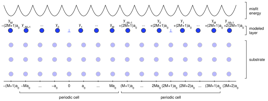
Figure 1. Frenkel-Kontorova model. The wells depict the misfit energy caused by the substrate.

The vector $\mathbf{y}=(y_{-M+1},\dots,y_{M})\in{\mathbb{R}}^{2M}$ describes the positions of $2M$ atoms which generate the positions of an infinite chain of atoms by the relation

$$y_{i+2M}=y_{i}+(2M+1)a_{0}\quad\text{for }i=-\infty,\dots,\infty,$$ (2.1)

where $a_{0}$ denotes the lattice constant. The relation (2.1) gives an average strain of $(2M+1)/2M$ due to a periodic array of dislocations that stretch the chain by one lattice constant every $2M$ atoms.

The total energy $\mathcal{E}^{a}$ for this atomistic system reads

$$\mathcal{E}^{a}(\mathbf{y})=\mathcal{E}^{a,e}(\mathbf{y})+\mathcal{E}^{a,m}(\mathbf{y})$$ (2.2)

with elastic energy given by (recall (2.1))

$$\begin{split}\mathcal{E}^{a,e}(\mathbf{y})&={\textstyle\frac{1}{2}}k_{1}\sum_{i=-M+1}^{M}(y_{i+1}-y_{i}-a_{0})^{2}+{\textstyle\frac{1}{2}}k_{2}\sum_{i=-M+2}^{M+1}(y_{i+1}-y_{i-1}-2a_{0})^{2}\\ &={\textstyle\frac{1}{2}}k_{1}\Bigg{[}\sum_{i=-M+1}^{M-1}(y_{i+1}-y_{i}-a_{0})^{2}+(y_{-M+1}-y_{M}+2Ma_{0})^{2}\Bigg{]}\\ &\quad+{\textstyle\frac{1}{2}}k_{2}\Bigg{[}\sum_{i=-M+2}^{M-1}(y_{i+1}-y_{i-1}-2a_{0})^{2}+(y_{-M+1}-y_{M-1}+(2M-1)a_{0})^{2}\\ &\hskip 180.67499pt+(y_{-M+2}-y_{M}+(2M-1)a_{0})^{2}\Bigg{]}\end{split}$$ (2.3)

and misfit energy given by

$$\mathcal{E}^{a,m}(\mathbf{y}) ={\textstyle\frac{1}{2}}k_{0}\sum_{i=-M+1}^{M}\left(y_{i}-a_{0}\left\lfloor\frac{y_{i}}{a_{0}}+\frac{1}{2}\right\rfloor\right)^{2}.$$ (2.4)

Here $k_{0}$, $k_{1}$ and $k_{2}$ denote the elastic constants. In the misfit energy, $\lfloor x\rfloor$ denotes the largest integer smaller than or equal to $x.$ We can obtain the following more symmetric form of the elastic energy (2.3) by realizing that the forces of constraint corresponding to the strain (2.1) move the equilibrium spacing of the chain to $\frac{2M+1}{2M}a_{0}:$

$$\begin{split}\mathcal{E}^{a,e}(\mathbf{y})&={\textstyle\frac{1}{2}}k_{1}\left[\sum_{i=-M+1}^{M}\Big{(}y_{i+1}-y_{i}-{\textstyle\frac{2M+1}{2M}}\big{(}\left(\left(i+1\right)\text{ mod }2M\right)-i\big{)}a_{0}\Big{)}^{2}+{\textstyle\frac{1}{2M}}a_{0}^{2}\right]\\ \qquad&+{\textstyle\frac{1}{2}}k_{2}\left[\sum_{i=-M+1}^{M}\Big{(}y_{i+2}-y_{i}-{\textstyle\frac{2M+1}{2M}}\big{(}\left(\left(i+2\right)\text{ mod }2M\right)-i\big{)}a_{0}\Big{)}^{2}+{\textstyle\frac{2}{M}}a_{0}^{2}\right]\end{split}$$ (2.5)

where all atom indices are understood modulo $2M$, and $i\text{ mod }2M$ denotes $i$ modulo $2M$ within the interval $-M+1,\ldots,M$. In the following, we neglect the constant terms since they do not have any effect when finding energy minimizers later.

We consider a single vacancy between the atoms $y_{0}$ and $y_{1}$. If we assume that the $M$ leftmost atoms $y_{i}$ for $-M+1\leq i\leq 0$ are situated in the interval $\left(\left(i-\frac{3}{2}\right)a_{0},\left(i-\frac{1}{2}\right)a_{0}\right)$ and that the $M$ rightmost atoms $y_{i}$ for $1\leq i\leq M$ are situated in the interval $\left(\left(i-\frac{1}{2}\right)a_{0},\left(i+\frac{1}{2}\right)a_{0}\right)$, then the misfit energy can be expressed more simply as

$$\mathcal{E}^{a,m}(\mathbf{y}) ={\textstyle\frac{1}{2}}k_{0}\sum_{i=-M+1}^{M}\left(y_{i}-b_{i}\right)^{2}\qquad\text{with}\qquad b_{i}=\begin{cases}(i-1)a_{0}&\text{for }i\leq 0,\\ ia_{0}&\text{for }i\geq 1.\end{cases}$$ (2.6)

To reduce the work in computing (2.2), we employ the quasicontinuum method [9, 10, 11] which has been successfully used for many applications. The quasicontinuum method consists of two steps: the passage to a continuum energy within the continuum region of the chain, and a subsequent coarsening in the continuum region to reduce the number of degrees of freedom.

In the first step, we replace the atomistic energy of all atoms from the continuum region by a continuum energy. To this end, we split the total energy into atom-wise contributions:

$$\mathcal{E}^{a}(\mathbf{y})=\sum_{i=-M+1}^{M}\mathcal{E}^{a,i}(\mathbf{y})$$ (2.7)

with

$$\begin{split}\mathcal{E}^{a,i}(\mathbf{y})=\quad{\textstyle\frac{1}{4}}k_{1}\Big{[}\quad&\left(y_{i}-y_{i-1}-{\textstyle\frac{2M+1}{2M}}\big{(}i-\left(\left(i-1\right)\text{ mod }2M\right)\big{)}a_{0}\right)^{2}\\ +&\left(y_{i+1}-y_{i}-{\textstyle\frac{2M+1}{2M}}\big{(}\left(\left(i+1\right)\text{ mod }2M\right)-i\big{)}a_{0}\right)^{2}\Big{]}\\ +{\textstyle\frac{1}{4}}k_{2}\Big{[}\quad&\left(y_{i}-y_{i-2}-{\textstyle\frac{2M+1}{2M}}\big{(}i-\left(\left(i-2\right)\text{ mod }2M\right)\big{)}a_{0}\right)^{2}\\ +&\left(y_{i+2}-y_{i}-{\textstyle\frac{2M+1}{2M}}\big{(}\left(\left(i+2\right)\text{ mod }2M\right)-i\big{)}a_{0}\right)^{2}\Big{]}\\ +{\textstyle\frac{1}{2}}k_{0}(y_{i}&-b_{i})^{2}.\end{split}$$ (2.8)

The corresponding continuum energy can be derived following [2] to be

$$\begin{split}\mathcal{E}^{c,i}(\mathbf{y})=\quad\left({\textstyle\frac{1}{4}}k_{1}+k_{2}\right)\Big{[}\quad&\left(y_{i}-y_{i-1}-{\textstyle\frac{2M+1}{2M}}\big{(}i-\left(\left(i-1\right)\text{ mod }2M\right)\big{)}a_{0}\right)^{2}\\ +&\left(y_{i+1}-y_{i}-{\textstyle\frac{2M+1}{2M}}\big{(}\left(\left(i+1\right)\text{ mod }2M\right)-i\big{)}a_{0}\right)^{2}\Big{]}\\ +{\textstyle\frac{1}{2}}k_{0}(y_{i}&-b_{i})^{2}.\end{split}$$ (2.9)

If

$$\delta_{i}^{a}=\begin{cases}1&\text{if atom $i$ is modeled atomistically,}\\ 0&\text{if atom $i$ is modeled as continuum,}\end{cases}\qquad\text{and}\qquad\delta_{i}^{c}=1-\delta_{i}^{a},$$ (2.10)

then

$$\mathcal{E}^{ac}(\mathbf{y})=\sum_{i=-M+1}^{M}\left[\delta^{a}_{i}\mathcal{E}^{a,i}(\mathbf{y})+\delta^{c}_{i}\mathcal{E}^{c,i}(\mathbf{y})\right]$$ (2.11)

denotes the mixed atomistic-continuum energy.

In the second step of the quasicontinuum approximation, the chain is coarsened in the continuum region by choosing representative atoms, more briefly called repatoms. The chain is then fully modeled in terms of the repatoms. The missing atoms are implicitly reconstructed by linear interpolation according to the Cauchy-Born hypothesis. The lengthy expression of the resulting quasicontinuum energy

$$\mathcal{E}^{qc}(\mathbf{y})$$ (2.12)

is not needed in this paper since we focus on the estimation of the modeling error. Hence we refer to [2] for the formula and its derivation. The error arising from coarsening will be studied in a forthcoming paper.

For the subsequent argumentation, it is useful to rewrite the energies in matrix notation. We have

$$\begin{split}\mathcal{E}^{a}(\mathbf{y})&={\textstyle\frac{1}{2}}(\mathbf{y}-\mathbf{a}^{a})^{T}D^{T}E^{a}D(\mathbf{y}-\mathbf{a}^{a})+{\textstyle\frac{1}{2}}(\mathbf{y}-\mathbf{b}^{a})^{T}K^{a}(\mathbf{y}-\mathbf{b}^{a}),\\ \mathcal{E}^{ac}(\mathbf{y})&={\textstyle\frac{1}{2}}(\mathbf{y}-\mathbf{a}^{a})^{T}D^{T}E^{ac}D(\mathbf{y}-\mathbf{a}^{a})+{\textstyle\frac{1}{2}}(\mathbf{y}-\mathbf{b}^{a})^{T}K^{a}(\mathbf{y}-\mathbf{b}^{a}),\end{split}$$ (2.13)

where the $2M\times 2M$ matrices are given by

$$\begin{array}[]{ll}D_{i,i}=-1,&D_{i,i+1}=1,\\ (E^{a})_{i,i}=k_{1}+2k_{2},&(E^{a})_{i,i+1}=(E^{a})_{i+1,i}=k_{2},\\ \lx@intercol(E^{ac})_{i,i}={\textstyle\frac{1}{2}}k_{1}\left(\delta^{a}_{i}+\delta^{a}_{i+1}\right)+{\textstyle\frac{1}{2}}k_{2}\left(\delta^{a}_{i-1}+\delta^{a}_{i}+\delta^{a}_{i+1}+\delta^{a}_{i+2}\right)+\left({\textstyle\frac{1}{2}}k_{1}+2k_{2}\right)\left(\delta^{c}_{i}+\delta^{c}_{i+1}\right),\hfil\lx@intercol\\ \lx@intercol(E^{ac})_{i,i+1}=(E^{ac})_{i+1,i}={\textstyle\frac{1}{2}}k_{2}\left(\delta^{a}_{i}+\delta^{a}_{i+2}\right),\hfil\lx@intercol\\ (K^{a})_{i,i}=k_{0},\end{array}$$ (2.14)

with $i=-M+1,\ldots,M$ and all indices to be understood modulo $2M$ as before. The vectors $\mathbf{a}^{a}\in{\mathbb{R}}^{2M}$ and $\mathbf{b}^{a}\in{\mathbb{R}}^{2M}$ are defined as

$$\begin{split}\mathbf{a}^{a}&=\begin{bmatrix}(-M+1){\textstyle\frac{2M+1}{2M}}a_{0}&(-M+2){\textstyle\frac{2M+1}{2M}}a_{0}&\cdots&(M-1){\textstyle\frac{2M+1}{2M}}a_{0}&M{\textstyle\frac{2M+1}{2M}}a_{0}\end{bmatrix}^{T},\\ \mathbf{b}^{a}&=\begin{bmatrix}b_{-M+1}&b_{-M+2}&\cdots&b_{M-1}&b_{M}\end{bmatrix}^{T}.\end{split}$$ (2.15)

We require that the elastic moduli satisfy $k_{1}+2k_{2}>2|k_{2}|$ to ensure that $E^{a}$ is positive definite and that the misfit modulus $k_{0}>0$ to ensure that $K^{a}$ is positive definite.

We are interested in finding energy minimizing configurations $\mathbf{y}^{a}$, $\mathbf{y}^{ac}$, and $\mathbf{y}^{qc}$ of $\mathcal{E}^{a}$, $\mathcal{E}^{ac}$, and $\mathcal{E}^{qc}$, respectively. The minimizers $\mathbf{y}^{a}$ and $\mathbf{y}^{ac}$ satisfy the linear equations

$$\begin{split}M^{a}\mathbf{y}^{a}&=\mathbf{f}^{a},\\ M^{ac}\mathbf{y}^{ac}&=\mathbf{f}^{ac},\end{split}$$ (2.16)

where

$$M^{a} :=D^{T}E^{a}D+K^{a}, \hskip 56.9055pt\mathbf{f}^{a} :=D^{T}E^{a}D\mathbf{a}^{a}+K^{a}\mathbf{b}^{a},$$ (2.17)

$$M^{ac} :=D^{T}E^{ac}D+K^{a}, \mathbf{f}^{ac} :=D^{T}E^{ac}D\mathbf{a}^{a}+K^{a}\mathbf{b}^{a}.$$

We refer to (2.16) as the primal problems. Note that the minimizers are uniquely determined due to the convexity of the energy.

3. Error Estimation

In the preceding section, we described how the quasicontinuum method gives an approximation $\mathbf{y}^{ac}$ of the atomistic solution $\mathbf{y}^{a}$ by passing from the fully atomistic model to a mixed atomistic-continuum formulation, and then we briefly mentioned how a further approximation, $\mathbf{y}^{qc}$, can be obtained by coarsening in the continuum region.

Instead of measuring the error in some global norm, we measure the error of a quantity of interest denoted by $Q(\mathbf{y})$ for some function $Q:{\mathbb{R}}^{2M}\to{\mathbb{R}}$. We assume that $Q$ is linear and thus has a representation

$$Q(\mathbf{y})=\mathbf{q}^{T}\mathbf{y}$$ (3.1)

for some vector $\mathbf{q}\in{\mathbb{R}}^{2M}$. We then have the splitting

$$|Q(\mathbf{y}^{a})-Q(\mathbf{y}^{qc})|=|Q(\mathbf{y}^{a}-\mathbf{y}^{ac})+Q(\mathbf{y}^{ac}-\mathbf{y}^{qc})|\leq|Q(\mathbf{y}^{a}-\mathbf{y}^{ac})|+|Q(\mathbf{y}^{ac}-\mathbf{y}^{qc})|$$ (3.2)

of the total error into the modeling error, $|Q(\mathbf{y}^{a}-\mathbf{y}^{ac})|$, and the coarsening error, $|Q(\mathbf{y}^{ac}-\mathbf{y}^{qc})|$, everything in terms of the quantity of interest. In this paper, we restrict ourselves to the estimation of the modeling error. The coarsening error will be analyzed in a forthcoming paper.

An important tool for the error estimation in terms of a quantity of interest are the dual problems for the influence or generalized Green’s functions $\mathbf{g}^{a}$ and $\mathbf{g}^{ac}$ given by

$$\begin{split}M^{a}\mathbf{g}^{a}&=\mathbf{q},\\ M^{ac}\mathbf{g}^{ac}&=\mathbf{q}.\end{split}$$ (3.3)

The matrices $M^{a}$ and $M^{ac}$ are symmetric since they stem from an energy, and we thus do not need to use their transpose for the dual problems.

We denote the errors and the residuals, both for the deformation $\mathbf{y}^{a}$ and the influence function $\mathbf{g}^{a},$ by

$$\mathbf{e} :=\mathbf{y}^{a}-\mathbf{y}^{ac}, \hskip 56.9055ptR(\mathbf{y}) :=M^{a}\left(\mathbf{y}^{a}-\mathbf{y}\right)=\mathbf{f}^{a}-M^{a}\mathbf{y},$$ (3.4)

$$\hat{\mathbf{e}} :=\mathbf{g}^{a}-\mathbf{g}^{ac}, \hat{R}(\mathbf{g}) :=M^{a}\left(\mathbf{g}^{a}-\mathbf{g}\right)=\mathbf{q}-M^{a}\mathbf{g}.$$

Then we have the basic identity for the error of the quantity of interest

$$\begin{split}Q(\mathbf{y}^{a})-Q(\mathbf{y}^{ac})&=\mathbf{q}^{T}\mathbf{e}=\mathbf{g}^{aT}M^{a}\mathbf{e}=(\mathbf{g}^{ac}+\hat{\mathbf{e}})^{T}M^{a}\mathbf{e}\\ &=\mathbf{g}^{acT}R(\mathbf{y}^{ac})+\hat{\mathbf{e}}^{T}M^{a}\mathbf{e}.\end{split}$$ (3.5)

The quantities $\mathbf{y}^{ac}$ and $\mathbf{g}^{ac}$ are considered to be computable since the continuum degrees of freedom give local interactions, whereas $\mathbf{y}^{a}$ and $\mathbf{g}^{a}$ are not considered to be computable since they require a full atomistic computation. Thus the first term $\mathbf{g}^{acT}R(\mathbf{y}^{ac})$ is easily computable, and the challenge is to estimate $\hat{\mathbf{e}}^{T}M^{a}\mathbf{e}$. Let us note that in applications to mesh refinement for linear finite elements, the residual term vanishes due to Galerkin orthogonality, whereas in other applications it can be dominant over the second term.

We utilize two error estimators derived in [2] and briefly summarized here. Our first error estimator is based on the generalized parallelogram identity

$$\hat{\mathbf{e}}^{T}M^{a}\mathbf{e}=\textstyle\frac{1}{4}\|\sigma\mathbf{e}+\sigma^{-1}\hat{\mathbf{e}}\|_{M^{a}}^{2}-\frac{1}{4}\|\sigma\mathbf{e}-\sigma^{-1}\hat{\mathbf{e}}\|_{M^{a}}^{2}$$ (3.6)

for all $\sigma\neq 0$, where the $M^{a}$-norm of some vector $\mathbf{z}$ is defined by $\|\mathbf{z}\|_{M^{a}}:=(\mathbf{z}^{T}M^{a}\mathbf{z})^{1/2}$. We define the computable bounds

$$\eta_{\text{low}}^{\pm}\leq\|\sigma\mathbf{e}\pm\sigma^{-1}\hat{\mathbf{e}}\|_{M^{a}}\leq\eta_{\text{upp}}^{\pm}$$ (3.7)

by

$$\eta_{\text{upp}}^{\pm} :=\big{\|}PD\big{[}\sigma(\mathbf{y}^{ac}-\mathbf{a}^{a})\pm\sigma^{-1}\mathbf{g}^{ac}\big{]}\big{\|}_{E^{a}},$$ (3.8)

$$\eta_{\text{low}}^{\pm} :=\frac{\left|(\mathbf{y}^{ac}+\theta^{\pm}\mathbf{g}^{ac})^{T}\mathbf{r}^{\pm}\right|}{\|\mathbf{y}^{ac}+\theta^{\pm}\mathbf{g}^{ac}\|_{M^{a}}}$$

where

$$P :=I-(E^{a})^{-1}E^{ac},$$ (3.9)

$$\mathbf{r}^{\pm} :=\sigma R(\mathbf{y}^{ac})\pm\sigma^{-1}\hat{R}(\mathbf{g}^{ac}).$$

Optimization of the bounds with respect to $\sigma$ and $\theta$ leads in [2] to the following choice of the parameters:

$$\begin{split}\sigma&:=\sqrt{\frac{\|PD\mathbf{g}^{ac}\|_{E^{a}}}{\|PD(\mathbf{y}^{ac}-\mathbf{a}^{a})\|_{E^{a}}}},\\ \theta^{\pm}&:=\frac{\mathbf{r}^{\pm T}\mathbf{y}^{ac}\;\mathbf{g}^{acT}M^{a}\mathbf{y}^{ac}-\mathbf{r}^{\pm T}\mathbf{g}^{ac}\;\|\mathbf{y}^{ac}\|_{M^{a}}^{2}}{\mathbf{r}^{\pm T}\mathbf{g}^{ac}\;\mathbf{g}^{acT}M^{a}\mathbf{y}^{ac}-\mathbf{r}^{\pm T}\mathbf{y}^{ac}\;\|\mathbf{g}^{ac}\|_{M^{a}}^{2}}.\end{split}$$ (3.10)

Theorem 3.1.

We have that

$$\left|Q(\mathbf{y}^{a})-Q(\mathbf{y}^{ac})\right|\leq\eta_{1},$$ (3.11)

where the computable error estimator $\eta_{1}$ is defined as

$$\textstyle\eta_{1}:=\max\left(\left|\mathbf{g}^{acT}R(\mathbf{y}^{ac})+\frac{1}{4}(\eta_{\text{low}}^{+})^{2}-\frac{1}{4}(\eta_{\text{upp}}^{-})^{2}\right|,\left|\mathbf{g}^{acT}R(\mathbf{y}^{ac})+\frac{1}{4}(\eta_{\text{upp}}^{+})^{2}-\frac{1}{4}(\eta_{\text{low}}^{-})^{2}\right|\right).$$ (3.12)

We also developed the following weaker estimator in [2] using the Cauchy-Schwarz inequality in place of the parallelogram identity in (3.6). We note that this estimator can be decomposed among the degrees of freedom and can thus be utilized in adaptive atomistic-continuum modeling decisions.

Theorem 3.2.

We have that

$$\left|Q(\mathbf{y}^{a})-Q(\mathbf{y}^{ac})\right|\leq\eta_{2}\leq\sum_{i=-M+1}^{M}\eta_{2,i}^{at}+\sum_{i=-M+1}^{M}\eta_{2,i}^{el}$$ (3.13)

where the computable global error estimator $\eta_{2}$ and the computable local error estimators $\eta_{2,i}^{at}$ and $\eta_{2,i}^{el}$, associated with atoms and elements, respectively, are defined as

$$\eta_{2}$$

(3.14)

4. Numerics

Now we use the two a posteriori error estimators given in Section 3 to formulate an algorithm which adaptively decides between atomistic and continuum modeling. Finally, we present and discuss the numerical results for the periodic array of dislocations described by the Frenkel-Kontorova model.

The error estimator $\eta_{1}$ gives a better estimate of the error because $\eta_{2}$ involves additional inequalities. However, $\eta_{2}$ allows for an atom-wise decomposition, whereas $\eta_{1}$ does not. This is due to the fact that $(\eta_{low}^{\pm})^{2}$ in the definition of $\eta_{1}$ is equal to the square of a sum of atom-wise components and not the sum of the square of these components. We can thus let $\eta_{1}$ decide whether a given global tolerance $\tau_{gl}$ is already achieved or not and use the decomposition of $\eta_{2}$ to decide where the atomistic model is needed for a better approximation. In this way, we combine the better efficiency of $\eta_{1}$ with the error localization of $\eta_{2}$.

We start with a fully continuum model. We then switch to the atomistic model wherever the local error exceeds an atom-wise error tolerance $\tau_{at}$. While decreasing $\tau_{at}$, the algorithm adaptively tags larger and larger regions atomistic until the estimate for the goal-oriented error finally reaches $\tau_{gl}$. The complete algorithm reads:

1. Choose $\tau_{gl}$. Model all atoms as a continuum. Set $\tau_{at}\leftarrow\tau_{gl}$.

2. Solve primal problem (2.16) for $\mathbf{y}^{ac}$ and dual problem (3.3) for $\mathbf{g}^{ac}$.

3. Compute error estimator $\eta_{1}$ from (3.12).

4. If $\eta_{1}\leq\tau_{gl},$ then stop.

5. Compute local error estimators $\eta_{2,i}^{at}$ and $\eta_{2,i}^{el}$ from (3.14).

6. Set $\tau_{at}\leftarrow\frac{\tau_{at}}{\tau_{div}}$.

7. Make all atoms $i$ atomistic ($\delta^{a}_{i}=1$ and $\delta^{c}_{i}=0$) for which

   $$\eta_{2,i}^{tot}:=\eta_{2,i}^{at}+{\textstyle\frac{1}{2}}\big{(}\eta_{2,i-1}^{el}+\eta_{2,i}^{el}\big{)}\geq\tau_{at}.$$ (4.1)

8. Go to (2).

The factor $\tau_{div}>1$ describes the rate at which the atom-wise tolerance $\tau_{at}$ is decreased during the adaptive process. We found that $\tau_{div}=10$ gives an efficient method for this problem.

Now we come to the results for the Frenkel-Kontorova dislocation model for a periodic chain of 1000 atoms, that is $M=500$. The elastic constants are set to be $k_{0}=1$ and $k_{1}=k_{2}=2$. To define the quantity of interest, we choose the average displacement of atoms $11\ldots 30$. This leads to

$$\mathbf{q}=(q_{i})_{i=-M+1,\ldots,M},\qquad q_{i}=1\quad\text{for }11\leq i\leq 30,\qquad q_{i}=0\quad\text{otherwise.}$$ (4.2)

The global tolerance is chosen to be $\tau_{gl}=10^{-10}$.

iteration	atomistic region	$\tau_{at}$	$\eta_{1}$
1	none	1.000000e-10	6.860546e-03
2	$-26\>\ldots\>55$	1.000000e-11	1.238016e-07
3	$-30\>\ldots\>60$	1.000000e-12	2.600112e-08
4	$-34\>\ldots\>66$	1.000000e-13	3.922946e-09
5	$-38\>\ldots\>73$	1.000000e-14	4.104868e-10
6	$-43\>\ldots\>80$	1.000000e-15	4.105166e-11

Table 1. Convergence of the algorithm for $\tau_{gl}=10^{-10}$.

Table 1 shows how the successive adaptive determination of the atomistic-continuum modeling proceeds. After six iterations, the atom-wise tolerance is small enough so that $\eta_{1}\leq\tau_{gl}$, that is the desired accuracy has been achieved.

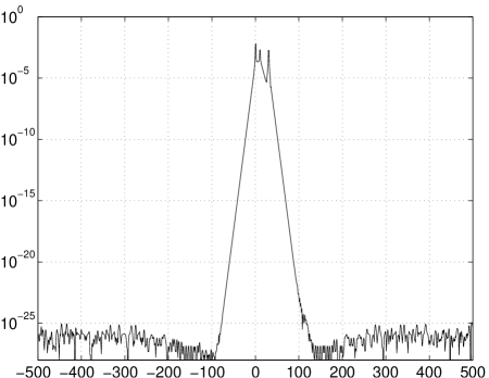
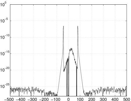
Figure 2. Decomposition of the error estimator $\eta_{2,i}^{tot}$ for iteration 1 (left, fully continuum model) and for iteration 6 (right, atomistic region $-43\ldots 80$).

Figure 2 shows the decomposition $\eta_{2,i}^{tot}$ of the error estimator $\eta_{2}$ for the fully continuum model in iteration 1 of the adaption process. One can clearly read off from the graph that the error is large near the dislocation between atoms 0 and 1 and near atoms 11 and 30, and that it decays exponentially away from these points. We note the slight nonsymmetry of the atomistic-continuum modeling due to using a goal function which averages over atoms $11\ldots 30$ to the right of the dislocation, but not to its left. The graph on the right shows the decomposition of $\eta_{2}$ in the final iteration 6 with an atomistic region given by indices $-43\dots 80$. It exhibits the same nonsymmetry, but the error is considerably smaller with peaks at the boundary between the atomistic region and the continuum region. In both diagrams, the fluctuations come from the limited relative machine precision of about $10^{-16}$.

atomistic
region			$|Q(\mathbf{y}^{a}-\mathbf{y}^{ac})|$	$\eta_{1}$	$\displaystyle\frac{\eta_{1}}{|Q(\mathbf{y}^{a}-\mathbf{y}^{ac})|}$	$\eta_{2}$	$\displaystyle\frac{\eta_{2}}{|Q(\mathbf{y}^{a}-\mathbf{y}^{ac})|}$
none			1.416421e-03	6.860545e-03	4.843577	1.231314e-02	8.693133
-4	$\>\>\ldots\>\>$	10	1.863104e-03	6.107510e-03	3.278136	1.049800e-02	5.634680
-9	$\>\>\ldots\>\>$	20	1.000572e-05	3.358722e-04	33.56803	6.621488e-04	66.17705
-14	$\>\>\ldots\>\>$	30	1.430363e-04	3.187552e-04	2.228492	5.140285e-04	3.593694
-19	$\>\>\ldots\>\>$	40	1.675490e-05	2.626711e-05	1.567727	3.691344e-05	2.203142
-24	$\>\>\ldots\>\>$	50	7.361419e-07	1.190138e-06	1.616723	1.693910e-06	2.301065
-29	$\>\>\ldots\>\>$	60	3.139276e-08	5.157753e-08	1.642975	7.388556e-08	2.353586
-34	$\>\>\ldots\>\>$	70	1.146997e-09	2.001550e-09	1.745035	2.934377e-09	2.558312

Table 2. Efficiency of the error estimators, $\eta_{1}/|Q(\mathbf{y}^{a}-\mathbf{y}^{ac})|$ and $\eta_{2}/|Q(\mathbf{y}^{a}-\mathbf{y}^{ac})|$.

Finally, Table 2 shows the efficiency of the error estimators $\eta_{1}$ and $\eta_{2}$ for different atomistic regions. $|Q(\mathbf{y}^{a}-\mathbf{y}^{ac})|$ gives the actual error which can be computed for this relatively small problem. In real applications, it is of course not available. One can clearly see that $\eta_{1}$ gives a better estimate than $\eta_{2}$, which numerically confirms our conjecture that $\eta_{1}$ is a better estimator than $\eta_{2}$. An unusually high value for the efficiency occurs when the atomistic-continuum boundary sweeps through the region where the quantity of interest is measured. After this, the efficiencies converge to decent values around 1.7 and 2.5 for $\eta_{1}$ and $\eta_{2}$, respectively. We note that for clamped boundary conditions and a symmetric quantity of interest, better efficiencies of 1.4 and 2, respectively, have been obtained [2].

References

[1]M. Ainsworth and J. T. Oden, A Posteriori Error Estimation in Finite
Element Analysis, Wiley, New York, 2000.
[2]M. Arndt and M. Luskin, Error estimation and atomistic-continuum
adaptivity for the quasicontinuum approximation of a Frenkel-Kontorova
model, 2007, arXiv:0704.1924.
[3]W. Bangerth and R. Rannacher, Adaptive Finite Element Methods for
Differential Equations, Lectures in Mathematics, ETH Zürich, Birkhäuser,
Basel, 2003.
[4]M. Dobson and M. Luskin, Analysis of a force-based quasicontinuum
approximation, 2006, arXiv:math.NA/0611543.
[5]M. Marder, Condensed Matter Physics, John Wiley & Sons, 2000.
[6]J. T. Oden, S. Prudhomme, and P. Bauman, Error control for molecular
statics problems, Int. J. Multiscale Comput. Eng., 4 (2006), pp. 647–662.
[7]J. T. Oden, S. Prudhomme, A. Romkes, and P. Bauman, Multiscale
modeling of physical phenomena: Adaptive control of models, SIAM J. Sci.
Comput., 28 (2006), pp. 2359–2389.
[8]J. T. Oden and K. S. Vemaganti, Estimation of local modeling error
and goal-oriented adaptive modeling of heterogeneous materials: Part I:
Error estimates and adaptive algorithms, J. Comput. Phys., 164 (2000),
pp. 22–47.
[9]E. B. Tadmor, R. Miller, R. Phillips, and M. Ortiz, Nanoindentation
and incipient plasticity, J. Mater. Res., 14 (1999), pp. 2233–2250.
[10]E. B. Tadmor, M. Ortiz, and R. Phillips, Quasicontinuum analysis of
defects in solids, Philos. Mag. A, 73 (1996), pp. 1529–1563.
[11]E. B. Tadmor, R. Phillips, and M. Ortiz, Mixed atomistic and
continuum models of deformation in solids, Langmuir, 12 (1996),
pp. 4529–4534.