Local three-nucleon interaction from chiral effective field theory

Abstract

The three-nucleon (NNN) interaction derived within the chiral effective field theory at the next-to-next-to-leading order (N²LO) is regulated with a function depending on the magnitude of the momentum transfer. The regulated NNN interaction is then local in the coordinate space, which is advantages for some many-body techniques. Matrix elements of the local chiral NNN interaction are evaluated in a three-nucleon basis. Using the ab initio no-core shell model (NCSM) the NNN matrix elements are employed in ³H and ⁴He bound-state calculations.

I Introduction

Interactions among nucleons are governed by quantum chromodynamics (QCD). In the low-energy regime relevant to nuclear structure, QCD is non-perturbative, and, therefore, hard to solve. Thus, theory has been forced to resort to models for the interaction, which have limited physical basis. New theoretical developments, however, allow us connect QCD with low-energy nuclear physics. The chiral effective field theory ($\chi$EFT) Weinberg provides a promising bridge. Beginning with the pionic or the nucleon-pion system bernard95 one works consistently with systems of increasing nucleon number ORK94 ; Bira ; bedaque02a . One makes use of spontaneous breaking of chiral symmetry to systematically expand the strong interaction in terms of a generic small momentum and takes the explicit breaking of chiral symmetry into account by expanding in the pion mass. Thereby, the NN interaction, the NNN interaction and also $\pi$N scattering are related to each other. At the same time, the pion mass dependence of the interaction is known, which will enable a connection to lattice QCD calculations in the future Beane06 . Nuclear interactions are non-perturbative, because diagrams with purely nucleonic intermediate states are enhanced Weinberg . Therefore, the chiral perturbation expansion is performed for the potential (note, however, the discussion in Refs. NTK05 ; Birse ; EM06 that points out some potential inconsitencies of this approach). Solving the Schrödinger equation for this potential then automatically sums diagrams with purely nucleonic intermediate states to all orders. The $\chi$EFT predicts, along with the NN interaction at the leading order, an NNN interaction at the 3rd order (next-to-next-to-leading order or N²LO) Weinberg ; vanKolck:1994 ; Epelbaum:2002 , and even an NNNN interaction at the 4th order (N³LO) Epelbaum06 . The details of QCD dynamics are contained in parameters, low-energy constants (LECs), not fixed by the symmetry. These parameters can be constrained by experiment. At present, high-quality NN potentials have been determined at order N³LO N3LO . A crucial feature of $\chi$EFT is the consistency between the NN, NNN and NNNN parts. As a consequence, at N²LO and N³LO, except for two LECs, assigned to two NNN diagrams, the potential is fully constrained by the parameters defining the NN interaction.

It is of great interest and also a challenge to apply the chiral interactions in nuclear structure and nuclear reaction calculations. In a recent work Navratil:2007 , the presently available NN potential at N³LO N3LO and the NNN interaction at N²LO vanKolck:1994 ; Epelbaum:2002 have been applied to the calculation of various properties of $s$- and $p$-shell nuclei, using the ab initio no-core shell model (NCSM) NCSMC12 ; NO03 , up to now the only approach able to handle the nonlocal $\chi$EFT NN potentials for systems beyond $A=4$. In that study, a preferred choice of the two NNN LECs, $c_{D}$ and $c_{E}$, was found and the fundamental importance of the $\chi$EFT NNN interaction was demonstrated for reproducing the structure of mid-$p$-shell nuclei. In a subsequent study, the same Hamiltonian was used to calculate microscopically the photo-absorption cross section of ⁴He Quaglioni:2007 .

The approach of Ref. Navratil:2007 differs in two aspects from the first NCSM application of the $\chi$EFT NN+NNN interactions in Ref. Nogga06 , which presents a detailed investigation of ⁷Li. First, a regulator depending on the momentum transfer in the NNN terms was introduced which results in a local $\chi$EFT NNN interaction. Second, the ⁴He binding energy was not used exclusively as the second constraint on the $c_{D}$ and $c_{E}$ LECs.

A local NNN interaction is advantages for some few- and many-body approaches because it is simpler to use. At the same time, it is known that details of the NNN interaction are important for nuclear structure applications. For example, the Urbana IX UIX and the Tucson-Melbourne TM ; TMp ; TMprime99 NNN interactions perform differently in mid-$p$-shell nuclei Pieper:04 ; GFMC_exc_6_8 ; NO03 although their differences appear to be minor. In the Green’s function Monte Carlo (GFMC) calculations with the AV18 NN potential AV18 , the best results for $p$-shell nuclei up to $A=10$ are found using the Illinois NNN interaction that augments the Urbana IX by a two-pion term from the Tucson-Melbourne NNN interaction and by three-pion terms that in the $\chi$EFT appear beyond the N³LO GFMC_IL ; GFMC_9_10 . Contrary to the Illinois NNN interaction, the $\chi$EFT NNN interaction features the above mentioned consistency with the accompanying NN interaction. Still, interestingly, we found that the nonlocal $\chi$EFT NNN interaction used in Ref. Nogga06 and the local $\chi$EFT NNN interaction employed in Ref. Navratil:2007 differ to some extent in their description of mid-$p$-shell nuclei with the latter giving results in a better agreement with experiment. Therefore, it is important to pay attention to the details of the NNN interaction and test different possibilities.

It is the purpose of this paper to elaborate on the details of the local $\chi$EFT NNN interaction used in Refs. Navratil:2007 ; Quaglioni:2007 and present its matrix elements in the three-nucleon basis. Technical details of dealing with NNN interactions were investigated in many papers CG81 ; Friar88 ; CP93 ; Huber97 ; Huber01 ; Barnea04 ; Adam04 . A new feature in the present work is the use of $\chi$EFT contact interactions and a focus on the application within the ab initio NCSM. In particular, we demonstrate the binding-energy convergence of the three-nucleon and four-nucleon systems with the $\chi$EFT NN+NNN interactions using the ab initio NCSM. In Sect. II, the local $\chi$EFT NNN interaction is discussed and compared to the nonlocal version of Ref. Epelbaum:2002 . Its three-nucleon matrix elements are given term by term. In Sect. III, the ³H and ⁴He binding energy and radius calculation results using the N³LO $\chi$EFT NN interaction of Ref. N3LO and the local $\chi$EFT NNN interaction are given. Conclusions are drawn in Sect. IV.

II Local $\chi$EFT NNN interaction at N²LO

The NNN interaction appearing at the third order (N²LO) of the $\chi$EFT comprises of three parts: (i) The two-pion exchange, (ii) the one-pion exchange plus contact and the three-nucleon contact. In this section, we discuss all the parts in detail and present the three-nucleon matrix elements of all the terms. For the two parts that contain the contact interactions, we also discuss in detail the impact of different regularization schemes.

II.1 Three-nucleon coordinates

We use the following definitions of the Jacobi coordinates

$$\vec{\xi}_{1} = \frac{1}{\sqrt{2}}(\vec{r}_{1}-\vec{r}_{2})\;,$$ (1)

$$\vec{\xi}_{2} = \sqrt{\frac{2}{3}}\left(\frac{1}{2}(\vec{r}_{1}+\vec{r}_{2})-\vec{r}_{3}\right)\;,$$ (2)

and associated momenta

$$\vec{\pi}_{1} = \frac{1}{\sqrt{2}}(\vec{p}_{1}-\vec{p}_{2})\;,$$ (3)

$$\vec{\pi}_{2} = \sqrt{\frac{2}{3}}\left(\frac{1}{2}(\vec{p}_{1}+\vec{p}_{2})-\vec{p}_{3}\right)\;.$$ (4)

We also define the momenta transferred by nucleon 2 and nucleon 3:

$$\vec{Q} = \vec{p}_{2}^{\prime}-\vec{p}_{2}=-\frac{1}{\sqrt{2}}(\vec{\pi}_{1}^{\prime}-\vec{\pi}_{1})+\frac{1}{\sqrt{6}}(\vec{\pi}_{2}^{\prime}-\vec{\pi}_{2})\;,$$ (5)

$$\vec{Q}^{\prime} = \vec{p}_{3}^{\prime}-\vec{p}_{3}=-\sqrt{\frac{2}{3}}(\vec{\pi}_{2}^{\prime}-\vec{\pi}_{2})\;,$$ (6)

where the primed coordinates refer to the initial momentum and the unprimed to the final momentum of the nucleon.

II.2 General structure of three-nucleon interaction and its matrix element

The NNN interaction is symmetric under permutation of the three nucleon indexes. It can be written as a sum of three pieces related by particle permutations:

$$W=W_{1}+W_{2}+W_{3}$$ (7)

To obtain its matrix element in an antisymmetrized three-nucleon basis we need to consider just a single term, e.g. $W_{1}$. In this paper, we use the basis of harmonic oscillator (HO) wave functions. However, most of the expressions have general validity. Following notation of Ref. TIHO:2000 , a general matrix element can be written as

$$\langle NiJT|W|N^{\prime}i^{\prime}JT\rangle=3\langle NiJT|W_{1}|N^{\prime}i^{\prime}JT\rangle = 3\sum\langle nlsjt,{\cal NLJ}||NiJT\rangle\langle n^{\prime}l^{\prime}s^{\prime}j^{\prime}t^{\prime},{\cal N^{\prime}L^{\prime}J^{\prime}}||N^{\prime}i^{\prime}JT\rangle$$ (8)

$$\times\langle(nlsjt,{\cal NLJ})JT|W_{1}|(n^{\prime}l^{\prime}s^{\prime}j^{\prime}t^{\prime},{\cal N^{\prime}L^{\prime}J^{\prime}})JT\rangle\;,$$

where $|NiJT\rangle$ is an antisymmetrized three-nucleon state with $N=2n+l+2{\cal N}+{\cal L}$, $i$ an additional quantum number and $J$ and $T$ the total angular momentum and total isospin, respectively. The parity of the state is $(-1)^{N}$. The state $|(nlsjt,{\cal NLJ})JT\rangle$ is a product of the HO wave functions $\langle\vec{\xi}_{1}|nl\rangle$ and $\langle\vec{\xi}_{2}|{\cal NL}\rangle$ associated with the coordinates (1) and (2), respectively. This state is antisymmetrized only with respect to the exchange of nucleons 1 and 2, i.e. $(-1)^{l+s+t}=-1$. The coefficient of fractional parentage $\langle nlsjt,{\cal NLJ}||NiJT\rangle$ is calculated according to Ref. TIHO:2000 .

II.3 N²LO three-nucleon interaction contact term

We start our discussion with the most trivial part of the $\chi$EFT N²LO NNN interaction, the three-nucleon contact term

$$W_{1}^{\rm cont} = E\vec{\tau}_{2}\cdot\vec{\tau}_{3}\delta(\vec{r}_{1}-\vec{r}_{2})\delta(\vec{r}_{3}-\vec{r}_{1})=E\vec{\tau}_{2}\cdot\vec{\tau}_{3}\frac{1}{(2\pi)^{6}}\frac{1}{(\sqrt{3})^{3}}\int{\rm d}\vec{\pi}_{1}{\rm d}\vec{\pi}_{2}{\rm d}\vec{\pi}_{1}^{\prime}{\rm d}\vec{\pi}_{2}^{\prime}|\vec{\pi}_{1}\vec{\pi}_{2}\rangle\langle\vec{\pi}_{1}^{\prime}\vec{\pi}_{2}^{\prime}|\;,$$ (9)

with $E=\frac{c_{E}}{F_{\pi}^{4}\Lambda_{\chi}}$ where $\Lambda_{\chi}$ is the chiral symmetry breaking scale of the order of the $\rho$ meson mass and $F_{\pi}=92.4$ MeV is the weak pion decay constant. The $c_{E}$ is a low-energy constant (LEC) from the chiral Lagrangian of order one. The corresponding diagram is shown in Fig. 1.

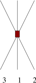
Figure 1: Contact interaction NNN term of the N²LO $\chi$EFT.

This term was regulated in Ref. Epelbaum:2002 by a regulator dependent on the sum of Jacobi momenta squared:

$$W_{1}^{\rm cont,ENGKMW} = E\vec{\tau}_{2}\cdot\vec{\tau}_{3}\frac{1}{(2\pi)^{6}}\frac{1}{(\sqrt{3})^{3}}\int{\rm d}\vec{\pi}_{1}{\rm d}\vec{\pi}_{2}{\rm d}\vec{\pi}_{1}^{\prime}{\rm d}\vec{\pi}_{2}^{\prime}|\vec{\pi}_{1}\vec{\pi}_{2}\rangle F(\textstyle{\frac{1}{2}(\pi_{1}^{2}+\pi_{2}^{2})};\Lambda)F(\textstyle{\frac{1}{2}}(\pi_{1}^{\prime 2}+\pi_{2}^{\prime 2});\Lambda)\langle\vec{\pi}_{1}^{\prime}\vec{\pi}_{2}^{\prime}|\;,$$ (10)

with the regulator function

$$F(q^{2};\Lambda)=\exp(-q^{4}/\Lambda^{4})$$ (11)

with the limit $F(q^{2};\Lambda\rightarrow\infty)=1$. This was in particular convenient as the calculations were performed in momentum space.

Alternatively, let us consider a regulator dependent on momentum transfer:

$$W_{1}^{\rm cont,Q} = E\vec{\tau}_{2}\cdot\vec{\tau}_{3}\frac{1}{(2\pi)^{6}}\frac{1}{(\sqrt{3})^{3}}\int{\rm d}\vec{\pi}_{1}{\rm d}\vec{\pi}_{2}{\rm d}\vec{\pi}_{1}^{\prime}{\rm d}\vec{\pi}_{2}^{\prime}|\vec{\pi}_{1}\vec{\pi}_{2}\rangle F(\vec{Q}^{2};\Lambda)F(\vec{Q}^{\prime 2};\Lambda)\langle\vec{\pi}_{1}^{\prime}\vec{\pi}_{2}^{\prime}|$$ (12)

$$= E\vec{\tau}_{2}\cdot\vec{\tau}_{3}\int{\rm d}\vec{\xi}_{1}{\rm d}\vec{\xi}_{2}|\vec{\xi}_{1}\vec{\xi}_{2}\rangle Z_{0}(\textstyle{\sqrt{2}}\xi_{1};\Lambda)Z_{0}(|\textstyle{\frac{1}{\sqrt{2}}}\vec{\xi}_{1}+\textstyle{\sqrt{\frac{3}{2}}}\vec{\xi}_{2}|;\Lambda)\langle\vec{\xi}_{1}\vec{\xi}_{2}|\;,$$

where we introduced the function

$$Z_{0}(r;\Lambda)=\frac{1}{2\pi^{2}}\int{\rm d}qq^{2}j_{0}(qr)F(q^{2};\Lambda)\;.$$ (13)

This results in an interaction local in coordinate space because of the dependence of the regulator function on differences of initial and final Jacobi momenta. An interaction local in coordinate space may be more convenient for some methods. In fact, most of the NNN interactions used in few-body calculations, such as the Tucson-Melbourne (TM^′) TMp ; TMprime99 , Urbana IX (UIX) UIX or Illinois 2 (IL2) GFMC_IL , are local in coordinate space.

The two alternatively regulated contact interactions lead to different three-nucleon matrix elements. The interaction (10) gives

$$\langle(nlsjt,{\cal NLJ})JT|W_{1}^{\rm cont,ENGKMW}|(n^{\prime}l^{\prime}s^{\prime}j^{\prime}t^{\prime},{\cal N^{\prime}L^{\prime}J^{\prime}})JT\rangle$$ (19)

$$= E\frac{1}{2\sqrt{3}\pi^{4}}\delta_{l0}\delta_{{\cal L}0}\delta_{l^{\prime}0}\delta_{{\cal L}^{\prime}0}\delta_{ss^{\prime}}\delta_{sj}\delta_{s^{\prime}j^{\prime}}\delta_{{\cal J}\frac{1}{2}}\delta_{{\cal J}^{\prime}\frac{1}{2}}\hat{t}\hat{t}^{\prime}(-1)^{t+t^{\prime}+T+\textstyle{\frac{1}{2}}}\left\{\begin{array}[]{ccc}t&t^{\prime}&1\\ \textstyle{\frac{1}{2}}&\textstyle{\frac{1}{2}}&\textstyle{\frac{1}{2}}\end{array}\right\}\left\{\begin{array}[]{ccc}t&t^{\prime}&1\\ \textstyle{\frac{1}{2}}&\textstyle{\frac{1}{2}}&T\end{array}\right\}$$

$$\times\int{\rm d}\pi_{1}{\rm d}\pi_{2}\pi_{1}^{2}\pi_{2}^{2}(-1)^{(n+{\cal N})}R_{n0}(\pi_{1},\textstyle{\frac{1}{b}})R_{{\cal N}0}(\pi_{2},\textstyle{\frac{1}{b}})F(\textstyle{\frac{1}{2}(\pi_{1}^{2}+\pi_{2}^{2})};\Lambda)$$

$$\times\int{\rm d}\pi_{1}^{\prime}{\rm d}\pi_{2}^{\prime}\pi_{1}^{\prime 2}\pi_{2}^{\prime 2}(-1)^{(n^{\prime}+{\cal N}^{\prime})}R_{n^{\prime}0}(\pi^{\prime}_{1},\textstyle{\frac{1}{b}})R_{{\cal N}^{\prime}0}(\pi^{\prime}_{2},\textstyle{\frac{1}{b}})F(\textstyle{\frac{1}{2}}(\pi_{1}^{\prime 2}+\pi_{2}^{\prime 2});\Lambda)\;,$$

while the interaction (12) results in the following matrix element:

$$\langle(nlsjt,{\cal NLJ})JT|W_{1}^{\rm cont,Q}|(n^{\prime}l^{\prime}s^{\prime}j^{\prime}t^{\prime},{\cal N^{\prime}L^{\prime}J^{\prime}})JT\rangle$$ (32)

$$= E6\delta_{ss^{\prime}}\hat{t}\hat{t}^{\prime}(-1)^{t+t^{\prime}+T+\textstyle{\frac{1}{2}}}\left\{\begin{array}[]{ccc}t&t^{\prime}&1\\ \textstyle{\frac{1}{2}}&\textstyle{\frac{1}{2}}&\textstyle{\frac{1}{2}}\end{array}\right\}\left\{\begin{array}[]{ccc}t&t^{\prime}&1\\ \textstyle{\frac{1}{2}}&\textstyle{\frac{1}{2}}&T\end{array}\right\}\hat{j}\hat{j}^{\prime}\hat{\cal J}\hat{\cal J}^{\prime}\hat{l}^{\prime}\hat{\cal L}^{\prime}(-1)^{J-\textstyle{\frac{1}{2}}+{\cal J}^{\prime}-{\cal J}+l+{\cal L}+s}$$

$$\times\sum_{X}(-1)^{X}\hat{X}^{2}\left\{\begin{array}[]{ccc}l^{\prime}&l&X\\ j&j^{\prime}&s\end{array}\right\}\left\{\begin{array}[]{ccc}j&j^{\prime}&X\\ {\cal J}^{\prime}&{\cal J}&J\end{array}\right\}\left\{\begin{array}[]{ccc}{\cal J}^{\prime}&{\cal J}&X\\ {\cal L}&{\cal L}^{\prime}&\textstyle{\frac{1}{2}}\end{array}\right\}(l^{\prime}0X0|l0)({\cal L}^{\prime}0X0|{\cal L}0)$$

$$\times\int{\rm d}\xi_{1}{\rm d}\xi_{2}\xi_{1}^{2}\xi_{2}^{2}R_{nl}(\xi_{1},\textstyle{b})R_{{\cal N}{\cal L}}(\xi_{2},\textstyle{b})R_{n^{\prime}l^{\prime}}(\xi_{1},\textstyle{b})R_{{\cal N}^{\prime}{\cal L}^{\prime}}(\xi_{2},\textstyle{b})Z_{0}(\textstyle{\sqrt{2}}\xi_{1};\Lambda)Z_{0,X}(\sqrt{\textstyle{\frac{1}{2}}}\xi_{1},\sqrt{\textstyle{\frac{3}{2}}}\xi_{2};\Lambda)\;.$$

In the above expressions, we have introduced the radial HO wave functions $R_{nl}$ with the oscillator parameter $b$ and, further, a new function

$$Z_{0,X}(r_{1},r_{2};\Lambda)=\frac{1}{2\pi^{2}}\int{\rm d}qq^{2}j_{X}(qr_{1})j_{X}(qr_{2})F(q^{2};\Lambda)\;.$$ (33)

We also introduced the customary abriviation $\hat{l}=\sqrt{2l+1}$. It should be noted that the two differently regulated contact interaction have different tensorial structure. One would perhaps expect that matrix elements of a local interaction will be easier to calculate. This is not the case for the discussed contact interaction. From Eq. (19) we can see that the term (10) acts only in $S$-waves. On the other hand, the local interaction (12) acts in higher partial waves as well as seen from Eq. (32). We display this schematically in Fig. 2 by breaking the symmetry of the pure contact interaction diagram (Fig. 1) and showing the finite range of the momentum transfer regulated interaction.

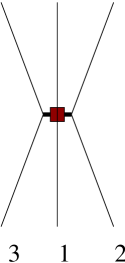
Figure 2: Contact interaction NNN term of the N²LO $\chi$EFT regulated by a function depending on momentum transfer.

Using $F(q^{2};\Lambda\rightarrow\infty)=1$, $Z_{0}(r,\Lambda\rightarrow\infty)=\frac{1}{4\pi r^{2}}\delta(r)$ and $Z_{0,X}(r_{1},r_{2};\Lambda\rightarrow\infty)=\frac{1}{4\pi r_{1}^{2}}\delta(r_{1}-r_{2})$, it is straightforward to verify that in the limit $\Lambda\rightarrow\infty$ both expressions (19) and (32) lead to the same result. For completeness, let us note that in Ref. Epelbaum:2002 a matrix element of $\vec{\tau}_{1}\cdot\vec{\tau}_{2}$ was calculated, i.e. $\langle\vec{\tau}_{1}\cdot\vec{\tau}_{2}\rangle=6\delta_{tt^{\prime}}(-1)^{t-1}\left\{\begin{array}[]{ccc}\textstyle{\frac{1}{2}}&\textstyle{\frac{1}{2}}&t\\ \textstyle{\frac{1}{2}}&\textstyle{\frac{1}{2}}&1\end{array}\right\}$, instead of $\vec{\tau}_{2}\cdot\vec{\tau}_{3}$ as we do in Eq. (19). Either choice lead to identical matrix element in the three-nucleon antisymmetrized basis (8). This is not the case once we regulate with the momentum transfer. Our choice in (12) results in the same isospin-coordinate structure as that obtained in Ref. vanKolck:1994 .

II.4 Transformation of the momentum part of the NNN interaction

A general NNN interaction term is a product of isospin, spin and momentum parts. In this subsection, we manipulate the momentum part. We only consider the case of the regulator function $F(q^{2},\Lambda)$ depending on transfered momentum. The momentum part of a general term $W_{1}$ can be schematically written as

$$g_{K_{1}}(|\vec{Q}|;\Lambda)g_{K_{2}}(|\vec{Q}^{\prime}|;\Lambda)(Y_{K_{1}}(\hat{Q})Y_{K_{2}}(\hat{Q}^{\prime}))^{(K)}\;,$$ (34)

with $K_{1}+K_{2}$ even and with $\vec{Q}$ and $\vec{Q}^{\prime}$ defined by Eqs. (3) and (4), respectively. For coordinates and momenta, $\hat{Q}$ denotes the angular part of the vector $\vec{Q}$. A transformation of (34) to coordinate space leads to a local interaction

$$\frac{1}{(2\pi)^{6}}\frac{1}{(\sqrt{3})^{3}}\int{\rm d}\vec{\pi}_{1}{\rm d}\vec{\pi}_{2}{\rm d}\vec{\pi}_{1}^{\prime}{\rm d}\vec{\pi}_{2}^{\prime}|\vec{\pi}_{1}\vec{\pi}_{2}\rangle g_{K_{1}}(|\vec{Q}|;\Lambda)g_{K_{2}}(|\vec{Q}^{\prime}|;\Lambda)(Y_{K_{1}}(\hat{Q})Y_{K_{2}}(\hat{Q}^{\prime}))^{(K)}\langle\vec{\pi}_{1}^{\prime}\vec{\pi}_{2}^{\prime}|$$ (35)

$$= i^{K_{1}+K_{2}}\int{\rm d}\vec{\xi}_{1}{\rm d}\vec{\xi}_{2}|\vec{\xi}_{1}\vec{\xi}_{2}\rangle f_{K_{1}}(\sqrt{2}\xi_{1};\Lambda)f_{K_{2}}(|\textstyle{\frac{1}{\sqrt{2}}}\vec{\xi}_{1}+\textstyle{\sqrt{\frac{3}{2}}}\vec{\xi}_{2}|;\Lambda)(Y_{K_{1}}(\hat{\xi}_{1})Y_{K_{2}}(\widehat{\textstyle{\frac{1}{\sqrt{2}}}\vec{\xi}_{1}+\textstyle{\sqrt{\frac{3}{2}}}\vec{\xi}_{2}}))^{(K)}\langle\vec{\xi}_{1}\vec{\xi}_{2}|\;.$$

Using (1) and (2), we note that $\sqrt{2}\vec{\xi}_{1}=\vec{r}_{1}-\vec{r}_{2}$ and $\textstyle{\frac{1}{\sqrt{2}}}\vec{\xi}_{1}+\textstyle{\sqrt{\frac{3}{2}}}\vec{\xi}_{2}=\vec{r}_{1}-\vec{r}_{3}$. In the above equation, we have introduced a new function using the relation

$$i^{K}f_{K}(r;\Lambda)Y_{Kk}(\hat{r})=\frac{1}{(2\pi)^{3}}\int{\rm d}\vec{q}\;\;{\rm e}^{i\vec{q}\cdot\vec{r}}g_{K}(q;\Lambda)Y_{Kk}(\hat{q})\;,$$ (36)

which implies

$$f_{K}(r;\Lambda)=\frac{1}{2\pi^{2}}\int{\rm d}qq^{2}j_{K}(qr)g_{K}(q;\Lambda)\;.$$ (37)

We manipulate Eq. (35) first by utilizing the spherical harmonics relation

$$Y_{K_{2}k_{2}}(\widehat{\vec{r}_{1}+\vec{r}_{2}})=\sum_{K_{3}=0}^{K_{2}}\frac{\sqrt{4\pi}}{\hat{K}_{3}}\left[\binom{2K_{2}+1}{2K_{3}}\right]^{\textstyle{\frac{1}{2}}}r_{1}^{K_{3}}r_{2}^{K_{2}-K_{3}}|\vec{r}_{1}+\vec{r}_{2}|^{-K_{2}}(Y_{K_{3}}(\hat{r}_{1})Y_{K_{2}-K_{3}}(\hat{r}_{2}))^{K_{2}}_{k_{2}}\;,$$ (38)

and, second, by the following expansion involving the functions depending on $|\textstyle{\frac{1}{\sqrt{2}}}\vec{\xi}_{1}+\textstyle{\sqrt{\frac{3}{2}}}\vec{\xi}_{2}|$:

$$f_{K_{2}}(|\vec{r}_{1}+\vec{r}_{2}|;\Lambda)|\vec{r}_{1}+\vec{r}_{2}|^{-K_{2}}=4\pi\sum_{XM_{X}}f_{K_{2},X}(r_{1},r_{2};\Lambda)(-1)^{X}Y^{*}_{XM_{X}}(\hat{r}_{1})Y_{XM_{X}}(\hat{r}_{2})\;,$$ (39)

with the function $f_{K_{2},X}(r_{1},r_{2};\Lambda)$ given by

$$f_{K_{2},X}(r_{1},r_{2};\Lambda)=\frac{2}{\pi}\int{\rm d}qq^{2}j_{X}(qr_{1})j_{X}(qr_{2})\int{\rm d}rr^{2}j_{0}(qr)\frac{f_{K_{2}}(r;\Lambda)}{r^{K_{2}}}\;,$$ (40)

or, equivalently, by

$$f_{K_{2},X}(r_{1},r_{2};\Lambda)=\textstyle{\frac{1}{2}}\int_{-1}^{1}{\rm d}uP_{X}(u)\frac{f_{K_{2}}(\sqrt{r_{1}^{2}+r_{2}^{2}-2r_{1}r_{2}u};\Lambda)}{(r_{1}^{2}+r_{2}^{2}-2r_{1}r_{2}u)^{K_{2}}}\;.$$ (41)

Using (38) and (39), the term (35) is re-written in the form

$$= i^{K_{1}+K_{2}}\int{\rm d}\vec{\xi}_{1}{\rm d}\vec{\xi}_{2}|\vec{\xi}_{1}\vec{\xi}_{2}\rangle f_{K_{1}}(\sqrt{2}\xi_{1};\Lambda)\sum_{K_{3}=0}^{K_{2}}\sum_{XYZV}\left[\binom{2K_{2}+1}{2K_{3}}\right]^{\textstyle{\frac{1}{2}}}(\textstyle{\frac{1}{\sqrt{2}}}\xi_{1})^{K_{3}}(\textstyle{\sqrt{\frac{3}{2}}}\xi_{2})^{K_{2}-K_{3}}f_{K_{2},X}(\textstyle{\frac{1}{\sqrt{2}}}\xi_{1},\textstyle{\sqrt{\frac{3}{2}}}\xi_{2};\Lambda)$$ (47)

$$\times\hat{X}^{2}\widehat{K_{2}-K_{3}}\hat{K}_{1}\hat{K}_{2}\hat{Y}(-1)^{K_{1}+Y+Z+K}\left\{\begin{array}[]{ccc}K_{1}&Y&V\\ Z&K&K_{2}\end{array}\right\}\left\{\begin{array}[]{ccc}Y&X&K_{3}\\ K_{2}-K_{3}&K_{2}&Z\end{array}\right\}$$

$$\times(X0K_{3}0|Y0)(X0K_{2}-K_{3}0|Z0)(Y0K_{1}0|V0)(Y_{V}(\hat{\xi}_{1})Y_{Z}(\hat{\xi}_{2}))^{(K)}_{k}\langle\vec{\xi}_{1}\vec{\xi}_{2}|\;,$$

which is convenient for matrix element calculations.

II.5 One-pion-exchange plus contact N²LO NNN term

We are now in a position to discuss the one-pion exchange plus contact term that appears at the N²LO. Following Ref. Epelbaum:2002 , we can write the $W_{1}$ term contribution as

$$W_{1}^{\rm 1\pi\_cont} = -D\frac{1}{(2\pi)^{6}}\frac{g_{\rm A}}{8F_{\pi}^{2}}\vec{\tau}_{2}\cdot\vec{\tau}_{3}\left[\frac{1}{\vec{Q}^{\prime 2}+M_{\pi}^{2}}\vec{\sigma}_{2}\cdot\vec{Q}^{\prime}\vec{\sigma}_{3}\cdot\vec{Q}^{\prime}+\frac{1}{\vec{Q}^{2}+M_{\pi}^{2}}\vec{\sigma}_{2}\cdot\vec{Q}\vec{\sigma}_{3}\cdot\vec{Q}\right]\;,$$ (48)

with $D=\frac{c_{D}}{F_{\pi}^{2}\Lambda_{\chi}}$, where $c_{D}$ is a LEC from the chiral Lagrangian of order one. A diagramatic depiction of the second term in the parenthesis is presented in Fig. 3. The first term corresponds to the exchange of $2\leftrightarrow 3$.

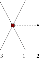
Figure 3: One-pion exchage plus contact NNN interaction term of the N²LO $\chi$EFT.

Using the regulator dependent on the sum of Jacobi momenta squared of Ref. Epelbaum:2002 , this term can be cast in the form

$$W_{1}^{\rm 1\pi\_cont,{\rm ENGKMW}} = -D\frac{1}{(2\pi)^{6}}\frac{g_{\rm A}}{8F_{\pi}^{2}}\frac{1}{(\sqrt{3})^{3}}\int{\rm d}\vec{\pi}_{1}{\rm d}\vec{\pi}_{2}{\rm d}\vec{\pi}_{1}^{\prime}{\rm d}\vec{\pi}_{2}^{\prime}|\vec{\pi}_{1}\vec{\pi}_{2}\rangle F(\textstyle{\frac{1}{2}(\pi_{1}^{2}+\pi_{2}^{2})};\Lambda)$$ (49)

$$\times\vec{\tau}_{2}\cdot\vec{\tau}_{3}\left[\frac{1}{\vec{Q}^{\prime 2}+M_{\pi}^{2}}\vec{\sigma}_{2}\cdot\vec{Q}^{\prime}\vec{\sigma}_{3}\cdot\vec{Q}^{\prime}+\frac{1}{\vec{Q}^{2}+M_{\pi}^{2}}\vec{\sigma}_{2}\cdot\vec{Q}\vec{\sigma}_{3}\cdot\vec{Q}\right]F(\textstyle{\frac{1}{2}}(\pi_{1}^{\prime 2}+\pi_{2}^{\prime 2});\Lambda)\langle\vec{\pi}_{1}^{\prime}\vec{\pi}_{2}^{\prime}|\;.$$

On the other hand, with a regulator dependent on momentum transfer, we get

$$W_{1}^{\rm 1\pi\_cont,{\rm Q}} = -D\frac{1}{(2\pi)^{6}}\frac{g_{\rm A}}{8F_{\pi}^{2}}\frac{1}{(\sqrt{3})^{3}}\int{\rm d}\vec{\pi}_{1}{\rm d}\vec{\pi}_{2}{\rm d}\vec{\pi}_{1}^{\prime}{\rm d}\vec{\pi}_{2}^{\prime}|\vec{\pi}_{1}\vec{\pi}_{2}\rangle F(\vec{Q}^{2};\Lambda)$$ (50)

$$\times\vec{\tau}_{2}\cdot\vec{\tau}_{3}\left[\frac{1}{\vec{Q}^{\prime 2}+M_{\pi}^{2}}\vec{\sigma}_{2}\cdot\vec{Q}^{\prime}\vec{\sigma}_{3}\cdot\vec{Q}^{\prime}+\frac{1}{\vec{Q}^{2}+M_{\pi}^{2}}\vec{\sigma}_{2}\cdot\vec{Q}\vec{\sigma}_{3}\cdot\vec{Q}\right]F(\vec{Q}^{\prime 2};\Lambda)\langle\vec{\pi}_{1}^{\prime}\vec{\pi}_{2}^{\prime}|\;,$$

which leads to a term local in coordinate space. We depict the second term in the parenthesis of (50) schematically in Fig. 4. The first term corresponds to the exchange of $2\leftrightarrow 3$. This choice of regulation results in spin-isopin-coordinate structure that also appears in NNN terms obtained in Ref. vanKolck:1994 . We note that a somewhat different spin-isopin structure was used for pion-range-short-range NNN terms in Refs. Huber01 and Adam04 . In Ref. Huber01 in particular, the $\vec{\sigma}$ and $\vec{\tau}$ operators were associated with the active nucleon 1, i.e.

$$W_{1}^{\rm 1\pi\_cont,{\rm Q}_{\sigma_{1}}} = -D\frac{1}{(2\pi)^{6}}\frac{g_{\rm A}}{8F_{\pi}^{2}}\frac{1}{(\sqrt{3})^{3}}\int{\rm d}\vec{\pi}_{1}{\rm d}\vec{\pi}_{2}{\rm d}\vec{\pi}_{1}^{\prime}{\rm d}\vec{\pi}_{2}^{\prime}|\vec{\pi}_{1}\vec{\pi}_{2}\rangle F(\vec{Q}^{2};\Lambda)$$ (51)

$$\times\left[\vec{\tau}_{1}\cdot\vec{\tau}_{3}\frac{1}{\vec{Q}^{\prime 2}+M_{\pi}^{2}}\vec{\sigma}_{1}\cdot\vec{Q}^{\prime}\vec{\sigma}_{3}\cdot\vec{Q}^{\prime}+\vec{\tau}_{1}\cdot\vec{\tau}_{2}\frac{1}{\vec{Q}^{2}+M_{\pi}^{2}}\vec{\sigma}_{1}\cdot\vec{Q}\vec{\sigma}_{2}\cdot\vec{Q}\right]F(\vec{Q}^{\prime 2};\Lambda)\langle\vec{\pi}_{1}^{\prime}\vec{\pi}_{2}^{\prime}|\;,$$

This change does not alter the matrix element of (49) in the antisymmetrized three-nucleon basis. It will lead to a difference in the matrix element of (50). However, the dependence on the regulator is a higher order effect than the $\chi$EFT expansion order used to derive the NNN interaction. Therefore, these differences should have only minor overall effect. In fact, we confirmed in nuclear structure calculations such as those described in Ref. Navratil:2007 that impact of the choice (49) or (50) is small in particular when the natural LECs values are used ($|c_{D}|\approx 1$). However, a more significant impact of the choice of the regulator in particular on spin-orbit force sensitive observables is observed in the case of the two-pion-exchange terms as discussed in the Introduction.

Figure 4: One-pion exchage plus contact NNN interaction term of the N²LO $\chi$EFT regulated by a function depending on momentum transfer.

Due to the antisymmetry of the three-nucleon wave functions in (8), it is sufficient to consider just one term of the two in parenthesis in (49) and (50) and multiply the result by two. Using the first term, the matrix element of (49) with the regulator dependent on the sum of Jacobi momenta squared is obtained in the form

$$\langle(nlsjt,{\cal NLJ})JT|W_{1}^{\rm 1\pi\_cont,{\rm ENGKMW}}|(n^{\prime}l^{\prime}s^{\prime}j^{\prime}t^{\prime},{\cal N^{\prime}L^{\prime}J^{\prime}})JT\rangle$$ (68)

$$= -D\frac{g_{\rm A}}{F_{\pi}^{2}}\frac{1}{2\sqrt{3}\pi^{4}}\delta_{l0}\delta_{l^{\prime}0}\delta_{sj}\delta_{s^{\prime}j^{\prime}}\hat{t}\hat{t}^{\prime}\left\{\begin{array}[]{ccc}t&t^{\prime}&1\\ \textstyle{\frac{1}{2}}&\textstyle{\frac{1}{2}}&\textstyle{\frac{1}{2}}\end{array}\right\}\left\{\begin{array}[]{ccc}t&t^{\prime}&1\\ \textstyle{\frac{1}{2}}&\textstyle{\frac{1}{2}}&T\end{array}\right\}(-1)^{(n+{\cal N}+n^{\prime}+{\cal N}^{\prime})+({\cal L}+{\cal L}^{\prime})/2}$$

$$\times\hat{j}\hat{j}^{\prime}\hat{\cal J}\hat{\cal J}^{\prime}(-1)^{J-{\cal J}+T+\textstyle{\frac{1}{2}}}\left\{\begin{array}[]{ccc}j&j^{\prime}&1\\ \textstyle{\frac{1}{2}}&\textstyle{\frac{1}{2}}&\textstyle{\frac{1}{2}}\end{array}\right\}\left\{\begin{array}[]{ccc}j&j^{\prime}&1\\ {\cal J}^{\prime}&{\cal J}&J\end{array}\right\}\sum_{K=0,2}\hat{K}(1010|K0)\left\{\begin{array}[]{ccc}{\cal J}&{\cal L}&\textstyle{\frac{1}{2}}\\ {\cal J}^{\prime}&{\cal L}^{\prime}&\textstyle{\frac{1}{2}}\\ 1&K&1\end{array}\right\}$$

$$\times\sum_{K_{1}=0}^{K}\widehat{K-K_{1}}\left[\binom{2K+1}{2K_{1}}\right]^{\textstyle{\frac{1}{2}}}(-1)^{{\cal L}+K_{1}}\sum_{X}\hat{X}\hat{\cal L}^{\prime}(K_{1}0X0|{\cal L}0)({\cal L}^{\prime}0K-K_{1}0|X0)\left\{\begin{array}[]{ccc}{\cal L}^{\prime}&K-K_{1}&X\\ K_{1}&{\cal L}&K\end{array}\right\}$$

$$\times\int{\rm d}\pi_{1}{\rm d}\pi_{2}{\rm d}\pi_{1}^{\prime}{\rm d}\pi_{2}^{\prime}\pi_{1}^{2}\pi_{2}^{2}\pi_{1}^{\prime 2}\pi_{2}^{\prime 2}R_{n0}(\pi_{1},\textstyle{\frac{1}{b}})R_{{\cal NL}}(\pi_{2},\textstyle{\frac{1}{b}})F(\textstyle{\frac{1}{2}(\pi_{1}^{2}+\pi_{2}^{2})};\Lambda)$$

$$\times R_{n^{\prime}0}(\pi^{\prime}_{1},\textstyle{\frac{1}{b}})R_{{\cal N}^{\prime}{\cal L}^{\prime}}(\pi^{\prime}_{2},\textstyle{\frac{1}{b}})F(\textstyle{\frac{1}{2}}(\pi_{1}^{\prime 2}+\pi_{2}^{\prime 2});\Lambda)\pi_{2}^{K_{1}}\pi_{2}^{\prime K-K_{1}}g_{K,X}(\pi_{2},\pi_{2}^{\prime})\;,$$

where we introduced the function

$$g_{K,X}(p,p^{\prime})=\frac{2}{\pi}\int{\rm d}qq^{2}drr^{2}\frac{q^{2-K}}{\textstyle{\frac{2}{3}}q^{2}+M_{\pi}^{2}}j_{0}(qr)j_{X}(pr)j_{X}(p^{\prime}r)\;,$$ (69)

which can be alternatively evaluated through

$$g_{K,X}(p,p^{\prime})=\textstyle{\frac{1}{2}}\int_{-1}^{1}{\rm d}uP_{X}(u)\frac{\sqrt{p^{2}+p^{\prime 2}-2pp^{\prime}u}^{2-K}}{\textstyle{\frac{2}{3}}(p^{2}+p^{\prime 2}-2pp^{\prime}u)^{2}+M_{\pi}^{2}}\;.$$ (70)

The matrix element (68) was first derived in Ref. Epelbaum:2002 .

For the one-pion exchange plus contact term (50) with the regulator dependent on momentum transfer, we present the matrix element obtained using both terms in the parenthesis of (50). Due to the three-nucleon wave function antisymmetry, both contributions lead to the same result for (8). One can take the advantage of this feature and use the alternative calculations to check the correctness of the numerical code. First, we take the first part of (50) and get

$$\langle(nlsjt,{\cal NLJ})JT|W_{1}^{\rm 1\pi\_cont,{\rm Q}}|(n^{\prime}l^{\prime}s^{\prime}j^{\prime}t^{\prime},{\cal N^{\prime}L^{\prime}J^{\prime}})JT\rangle$$ (92)

$$= -D\frac{9g_{\rm A}}{F_{\pi}^{2}}\hat{t}\hat{t}^{\prime}(-1)^{t+t^{\prime}+T+\textstyle{\frac{1}{2}}}\left\{\begin{array}[]{ccc}t&t^{\prime}&1\\ \textstyle{\frac{1}{2}}&\textstyle{\frac{1}{2}}&\textstyle{\frac{1}{2}}\end{array}\right\}\left\{\begin{array}[]{ccc}t&t^{\prime}&1\\ \textstyle{\frac{1}{2}}&\textstyle{\frac{1}{2}}&T\end{array}\right\}\hat{j}\hat{j}^{\prime}\hat{\cal J}\hat{\cal J}^{\prime}(-1)^{J-{\cal J}+s+j^{\prime}}\left\{\begin{array}[]{ccc}s&s^{\prime}&1\\ \textstyle{\frac{1}{2}}&\textstyle{\frac{1}{2}}&\textstyle{\frac{1}{2}}\end{array}\right\}$$

$$\times\sum_{K=0,2}\hat{K}(-1)^{(K/2)}(1010|K0)\sum_{K_{2},K_{3}}\hat{K}_{2}\hat{K}_{3}\hat{l}^{\prime}\hat{\cal L}^{\prime}(l^{\prime}0K_{2}0|l0)({\cal L}^{\prime}0K_{3}0|{\cal L}0)$$

$$\times\sum_{Z}\hat{Z}^{2}\left\{\begin{array}[]{ccc}l&s&j\\ l^{\prime}&s^{\prime}&j^{\prime}\\ K_{2}&1&Z\end{array}\right\}\left\{\begin{array}[]{ccc}{\cal L}&\textstyle{\frac{1}{2}}&{\cal J}\\ {\cal L}^{\prime}&\textstyle{\frac{1}{2}}&{\cal J}^{\prime}\\ K_{3}&1&Z\end{array}\right\}\left\{\begin{array}[]{ccc}j&j^{\prime}&Z\\ {\cal J}^{\prime}&{\cal J}&J\end{array}\right\}\left\{\begin{array}[]{ccc}K_{2}&1&Z\\ 1&K_{3}&K\end{array}\right\}$$

$$\times\sum_{K_{1}=0}^{K}\widehat{K-K_{1}}\left[\binom{2K+1}{2K_{1}}\right]^{\textstyle{\frac{1}{2}}}(-1)^{K_{1}}\sum_{X}(-1)^{X}\hat{X}^{2}(K_{1}0X0|K_{2}0)(K-K_{1}0X0|K_{3}0)\left\{\begin{array}[]{ccc}K_{1}&X&K_{2}\\ K_{3}&K&K-K_{1}\end{array}\right\}$$

$$\times\int{\rm d}\xi_{1}{\rm d}\xi_{2}\xi_{1}^{2}\xi_{2}^{2}R_{nl}(\xi_{1},\textstyle{b})R_{{\cal N}{\cal L}}(\xi_{2},\textstyle{b})R_{n^{\prime}l^{\prime}}(\xi_{1},\textstyle{b})R_{{\cal N}^{\prime}{\cal L}^{\prime}}(\xi_{2},\textstyle{b})$$

$$\times(\sqrt{\textstyle{\frac{1}{2}}}\xi_{1})^{K_{1}}(\sqrt{\textstyle{\frac{3}{2}}}\xi_{2})^{K-K_{1}}Z_{0}(\textstyle{\sqrt{2}}\xi_{1};\Lambda)f_{K,X}(\sqrt{\textstyle{\frac{1}{2}}}\xi_{1},\sqrt{\textstyle{\frac{3}{2}}}\xi_{2};\Lambda)\;,$$

with the functions

$$f_{0,X}(r_{1},r_{2};\Lambda)=\frac{1}{2\pi^{2}}\int{\rm d}qq^{2}j_{X}(qr_{1})j_{X}(qr_{2})\frac{q^{2}F(q^{2};\Lambda)}{q^{2}+M_{\pi}^{2}}\;,$$ (93)

and

$$f_{2,X}(r_{1},r_{2};\Lambda)=\frac{1}{4\pi^{2}}\int_{0}^{\infty}{\rm d}qq^{2}j_{X}(qr_{1})j_{X}(qr_{2})\int_{q}^{\infty}{\rm d}kk(k^{2}-q^{2})\frac{F(k^{2};\Lambda)}{k^{2}+M_{\pi}^{2}}\;,$$ (94)

which are special cases of (40). An alternative way of evaluating (94) is

$$f_{2,X}(r_{1},r_{2};\Lambda)=\textstyle{\frac{1}{2}}\int_{-1}^{1}{\rm d}uP_{X}(u)\frac{f_{2}(\sqrt{r_{1}^{2}+r_{2}^{2}-2r_{1}r_{2}u};\Lambda)}{r_{1}^{2}+r_{2}^{2}-2r_{1}r_{2}u}\;,$$ (95)

with

$$f_{2}(r;\Lambda)=\frac{1}{2\pi^{2}}\int{\rm d}qq^{2}j_{2}(qr)\frac{q^{2}F(q^{2};\Lambda)}{q^{2}+M_{\pi}^{2}}\;.$$ (96)

We note that (95) is numerically more efficient than (94).

Next, we take the second part of (50), which results in a simpler expression for one-pion-exchange plus contact N²LO three-nucleon matrix element in non-antisymmetrized basis:

$$\langle(nlsjt,{\cal NLJ})JT|W_{1}^{\rm 1\pi\_cont,{\rm Q}}|(n^{\prime}l^{\prime}s^{\prime}j^{\prime}t^{\prime},{\cal N^{\prime}L^{\prime}J^{\prime}})JT\rangle$$ (115)

$$= -D\frac{9g_{\rm A}}{F_{\pi}^{2}}\hat{t}\hat{t}^{\prime}(-1)^{t+t^{\prime}+T+\textstyle{\frac{1}{2}}}\left\{\begin{array}[]{ccc}t&t^{\prime}&1\\ \textstyle{\frac{1}{2}}&\textstyle{\frac{1}{2}}&\textstyle{\frac{1}{2}}\end{array}\right\}\left\{\begin{array}[]{ccc}t&t^{\prime}&1\\ \textstyle{\frac{1}{2}}&\textstyle{\frac{1}{2}}&T\end{array}\right\}\hat{j}\hat{j}^{\prime}\hat{\cal J}\hat{\cal J}^{\prime}\hat{s}\hat{s}^{\prime}(-1)^{J-{\cal J}+s+j^{\prime}}\left\{\begin{array}[]{ccc}s&s^{\prime}&1\\ \textstyle{\frac{1}{2}}&\textstyle{\frac{1}{2}}&\textstyle{\frac{1}{2}}\end{array}\right\}\hat{l}^{\prime}\hat{\cal L}^{\prime}$$

$$\times\sum_{K=0,2}\hat{K}(-1)^{(K/2)}(1010|K0)\sum_{V}(-1)^{V}\hat{V}(V0l^{\prime}0|l0)\sum_{X}\hat{X}^{2}(X0K0|V0)(X0{\cal L}^{\prime}0|{\cal L}0)$$

$$\times\sum_{Z}\hat{Z}^{2}\left\{\begin{array}[]{ccc}l&s&j\\ l^{\prime}&s^{\prime}&j^{\prime}\\ V&1&Z\end{array}\right\}\left\{\begin{array}[]{ccc}{\cal L}&\textstyle{\frac{1}{2}}&{\cal J}\\ {\cal L}^{\prime}&\textstyle{\frac{1}{2}}&{\cal J}^{\prime}\\ X&1&Z\end{array}\right\}\left\{\begin{array}[]{ccc}j&j^{\prime}&Z\\ {\cal J}^{\prime}&{\cal J}&J\end{array}\right\}\left\{\begin{array}[]{ccc}V&1&Z\\ 1&X&K\end{array}\right\}$$

$$\times\int{\rm d}\xi_{1}{\rm d}\xi_{2}\xi_{1}^{2}\xi_{2}^{2}R_{nl}(\xi_{1},\textstyle{b})R_{{\cal N}{\cal L}}(\xi_{2},\textstyle{b})R_{n^{\prime}l^{\prime}}(\xi_{1},\textstyle{b})R_{{\cal N}^{\prime}{\cal L}^{\prime}}(\xi_{2},\textstyle{b})f_{K}(\textstyle{\sqrt{2}}\xi_{1};\Lambda)Z_{0,X}(\sqrt{\textstyle{\frac{1}{2}}}\xi_{1},\sqrt{\textstyle{\frac{3}{2}}}\xi_{2};\Lambda)\;,$$

with

$$f_{K}(r;\Lambda)=\frac{1}{2\pi^{2}}\int{\rm d}qq^{2}j_{K}(qr)\frac{q^{2}F(q^{2};\Lambda)}{q^{2}+M_{\pi}^{2}}\;,$$ (116)

which is a special case of (37) and $Z_{0,X}(r_{1},r_{2};\Lambda)$ given by Eq. (33). Both (92) and (115) are already multiplied by two in anticipation of the three-nucleon antisymmetry in the final matrix element (8).

For completeness, we also present the matrix element of the second part of (51):

$$\langle(nlsjt,{\cal NLJ})JT|W_{1}^{\rm 1\pi\_cont,{\rm Q}_{\sigma_{1}}}|(n^{\prime}l^{\prime}s^{\prime}j^{\prime}t^{\prime},{\cal N^{\prime}L^{\prime}J^{\prime}})JT\rangle$$ (132)

$$= -D\frac{9g_{\rm A}}{F_{\pi}^{2}}\delta_{tt^{\prime}}(-1)^{t-1}\left\{\begin{array}[]{ccc}\textstyle{\frac{1}{2}}&\textstyle{\frac{1}{2}}&t\\ \textstyle{\frac{1}{2}}&\textstyle{\frac{1}{2}}&1\end{array}\right\}\hat{j}\hat{j}^{\prime}\hat{\cal J}\hat{\cal J}^{\prime}\hat{s}\hat{s}^{\prime}\hat{l}^{\prime}\hat{\cal L}^{\prime}(-1)^{s+s^{\prime}+j^{\prime}+J+{\cal L}+{\cal J}+{\cal J}^{\prime}+\textstyle{\frac{1}{2}}}$$

$$\times\sum_{K=0,2}\hat{K}(-1)^{(K/2)}(1010|K0)\left\{\begin{array}[]{ccc}s&s^{\prime}&K\\ \textstyle{\frac{1}{2}}&\textstyle{\frac{1}{2}}&1\\ \textstyle{\frac{1}{2}}&\textstyle{\frac{1}{2}}&1\end{array}\right\}\sum_{V}\hat{V}(V0l^{\prime}0|l0)\sum_{X}\hat{X}^{2}(X0K0|V0)(X0{\cal L}^{\prime}0|{\cal L}0)$$

$$\times\left\{\begin{array}[]{ccc}l&s&j\\ l^{\prime}&s^{\prime}&j^{\prime}\\ V&K&X\end{array}\right\}\left\{\begin{array}[]{ccc}{\cal J}&X&{\cal J}^{\prime}\\ j^{\prime}&J&j\end{array}\right\}\left\{\begin{array}[]{ccc}{\cal J}&X&{\cal J}^{\prime}\\ {\cal L}^{\prime}&\textstyle{\frac{1}{2}}&{\cal L}\end{array}\right\}$$

$$\times\int{\rm d}\xi_{1}{\rm d}\xi_{2}\xi_{1}^{2}\xi_{2}^{2}R_{nl}(\xi_{1},\textstyle{b})R_{{\cal N}{\cal L}}(\xi_{2},\textstyle{b})R_{n^{\prime}l^{\prime}}(\xi_{1},\textstyle{b})R_{{\cal N}^{\prime}{\cal L}^{\prime}}(\xi_{2},\textstyle{b})f_{K}(\textstyle{\sqrt{2}}\xi_{1};\Lambda)Z_{0,X}(\sqrt{\textstyle{\frac{1}{2}}}\xi_{1},\sqrt{\textstyle{\frac{3}{2}}}\xi_{2};\Lambda)\;,$$

which is still simpler than (115). Again, this matrix element is already multiplied by two in anticipation of the three-nucleon antisymmetry in the final matrix element (8). The matrix element of the (two-times the) first part of (51) is given by (92) multiplied by $(-1)^{t+t^{\prime}+s+s^{\prime}}$. Due to the three-nucleon wave function antisymmetry, this contribution leads to the same result for (8) as does (115), which can be taken advantage of in testing the correctness of numerical calculations.

By comparing (49) with (92) (or equivalently with (115) and also with (132)) we note the different tensorial structure of the matrix elements. When the regulator dependent on the sum of Jacobi momenta squared is used, only the $l=0$, $l^{\prime}=0$ partial waves contribute. This is not the case, when the regulator depending on momentum transfer is utilized. At the same time, however, we note that in the limit $\Lambda\rightarrow\infty$ both expressions (49) and (92) as well as (115) and (132) lead to the same result.

II.6 Two-pion exchange N²LO NNN terms

In this subsection, we present matrix elements of two-pion exchange N²LO NNN terms. Their schematic depiction is shown in Fig. 5.

Figure 5: Two-pion exchange NNN interaction term of the N²LO $\chi$EFT.

There are three distinct terms associated with three LECs, $c_{1}$, $c_{3}$ and $c_{4}$, from the chiral Lagrangian, which also appear in the subleading two-pion exchange in the NN potential. Consequently, values of these LECs expected to be of order one are typically fixed at the NN level unlike the case of the previously introduced $c_{D}$ (48) and $c_{E}$ (9) LECs whose values needs to be fixed in systems of more than two nucleons. In the present paper, we derive only the matrix elements of the two-pion exchange NNN interaction terms regulated by a function depending on momentum transfer, i.e. terms that are local in coordinate space.

Following Ref. Epelbaum:2002 , the $W_{1}$ part of the $c_{1}$ term with the momentum transfer regulators can be written as

$$W_{1}^{\rm 2\pi\_c1} = -c_{1}\frac{1}{(2\pi)^{6}}\frac{4M_{\pi}^{2}}{F_{\pi}^{2}}\frac{g_{\rm A}^{2}}{4F_{\pi}^{2}}\vec{\tau}_{2}\cdot\vec{\tau}_{3}F(\vec{Q}^{2};\Lambda)\frac{1}{\vec{Q}^{2}+M_{\pi}^{2}}\vec{\sigma}_{2}\cdot\vec{Q}\vec{\sigma}_{3}\cdot\vec{Q}^{\prime}\frac{1}{\vec{Q}^{\prime 2}+M_{\pi}^{2}}F(\vec{Q}^{\prime 2};\Lambda)\;.$$ (133)

Using results of Subsect. II.4, we find for the $c_{1}$-term matrix element:

$$\langle(nlsjt,{\cal NLJ})JT|W_{1}^{\rm 2\pi\_c1,{\rm Q}}|(n^{\prime}l^{\prime}s^{\prime}j^{\prime}t^{\prime},{\cal N^{\prime}L^{\prime}J^{\prime}})JT\rangle$$ (153)

$$= -c_{1}\frac{36M_{\pi}^{2}}{F_{\pi}^{2}}\frac{g_{\rm A}^{2}}{F_{\pi}^{2}}\hat{t}\hat{t}^{\prime}(-1)^{t+t^{\prime}+T+\textstyle{\frac{1}{2}}}\left\{\begin{array}[]{ccc}t&t^{\prime}&1\\ \textstyle{\frac{1}{2}}&\textstyle{\frac{1}{2}}&\textstyle{\frac{1}{2}}\end{array}\right\}\left\{\begin{array}[]{ccc}t&t^{\prime}&1\\ \textstyle{\frac{1}{2}}&\textstyle{\frac{1}{2}}&T\end{array}\right\}\hat{j}\hat{j}^{\prime}\hat{\cal J}\hat{\cal J}^{\prime}\hat{s}\hat{s}^{\prime}(-1)^{J-{\cal J}+s+j^{\prime}}\left\{\begin{array}[]{ccc}s&s^{\prime}&1\\ \textstyle{\frac{1}{2}}&\textstyle{\frac{1}{2}}&\textstyle{\frac{1}{2}}\end{array}\right\}\hat{l}^{\prime}\hat{\cal L}^{\prime}$$

$$\times\sum_{VR}\hat{V}\hat{R}(V0l^{\prime}0|l0)(R0{\cal L}^{\prime}0|{\cal L}0)\sum_{Y}(-1)^{Y}\hat{Y}(Y010|V0)\left\{\begin{array}[]{ccc}l&s&j\\ l^{\prime}&s^{\prime}&j^{\prime}\\ V&1&Y\end{array}\right\}\left\{\begin{array}[]{ccc}{\cal L}&\textstyle{\frac{1}{2}}&{\cal J}\\ {\cal L}^{\prime}&\textstyle{\frac{1}{2}}&{\cal J}^{\prime}\\ R&1&Y\end{array}\right\}\left\{\begin{array}[]{ccc}j&j^{\prime}&Y\\ {\cal J}^{\prime}&{\cal J}&J\end{array}\right\}$$

$$\times\sum_{K_{3}=0}^{1}\left[\binom{3}{2K_{3}}\right]^{\textstyle{\frac{1}{2}}}\widehat{1-K_{3}}\sum_{X}\hat{X}^{2}(X0K_{3}0|Y0)(X01-K_{3}0|R0)\left\{\begin{array}[]{ccc}Y&X&K_{3}\\ 1-K_{3}&1&R\end{array}\right\}$$

$$\times\int{\rm d}\xi_{1}{\rm d}\xi_{2}\xi_{1}^{2}\xi_{2}^{2}R_{nl}(\xi_{1},\textstyle{b})R_{{\cal N}{\cal L}}(\xi_{2},\textstyle{b})R_{n^{\prime}l^{\prime}}(\xi_{1},\textstyle{b})R_{{\cal N}^{\prime}{\cal L}^{\prime}}(\xi_{2},\textstyle{b})$$

$$\times(\sqrt{\textstyle{\frac{1}{2}}}\xi_{1})^{K_{3}}(\sqrt{\textstyle{\frac{3}{2}}}\xi_{2})^{1-K_{3}}f_{1}(\textstyle{\sqrt{2}}\xi_{1};\Lambda)f_{1,X}(\sqrt{\textstyle{\frac{1}{2}}}\xi_{1},\sqrt{\textstyle{\frac{3}{2}}}\xi_{2};\Lambda)\;.$$

Here we introduced the functions

$$f_{1}(r;\Lambda)=\frac{1}{2\pi^{2}}\int{\rm d}qq^{2}j_{1}(q)\frac{qF(q^{2};\Lambda)}{q^{2}+M_{\pi}^{2}}\;,$$ (154)

and

$$f_{1,X}(r_{1},r_{2};\Lambda)=\frac{1}{2\pi^{2}}\int_{0}^{\infty}{\rm d}qq^{2}j_{X}(qr_{1})j_{X}(qr_{2})\int_{q}^{\infty}{\rm d}k\frac{kF(k^{2};\Lambda)}{k^{2}+M_{\pi}^{2}}\;,$$ (155)

which are the explicit versions of functions given in Eqs. (37) and (40), respectively. The function (155) can be alternatively evaluated with the help of the Legendre polynomial:

$$f_{1,X}(r_{1},r_{2};\Lambda)=\textstyle{\frac{1}{2}}\int_{-1}^{1}{\rm d}uP_{X}(u)\frac{f_{1}(\sqrt{r_{1}^{2}+r_{2}^{2}-2r_{1}r_{2}u};\Lambda)}{\sqrt{r_{1}^{2}+r_{2}^{2}-2r_{1}r_{2}u}}\;.$$ (156)

The $W_{1}$ part of the two-pion exchange $c_{3}$ term is given by Epelbaum:2002

$$W_{1}^{\rm 2\pi\_c3} = c_{3}\frac{1}{(2\pi)^{6}}\frac{2}{F_{\pi}^{2}}\frac{g_{\rm A}^{2}}{4F_{\pi}^{2}}\vec{\tau}_{2}\cdot\vec{\tau}_{3}F(\vec{Q}^{2};\Lambda)\frac{1}{\vec{Q}^{2}+M_{\pi}^{2}}\vec{\sigma}_{2}\cdot\vec{Q}\vec{\sigma}_{3}\cdot\vec{Q}^{\prime}\vec{Q}\cdot\vec{Q}^{\prime}\frac{1}{\vec{Q}^{\prime 2}+M_{\pi}^{2}}F(\vec{Q}^{\prime 2};\Lambda)\;.$$ (157)

For its matrix element we find

$$\langle(nlsjt,{\cal NLJ})JT|W_{1}^{\rm 2\pi\_c3,{\rm Q}}|(n^{\prime}l^{\prime}s^{\prime}j^{\prime}t^{\prime},{\cal N^{\prime}L^{\prime}J^{\prime}})JT\rangle$$ (181)

$$= c_{3}\frac{18}{F_{\pi}^{2}}\frac{g_{\rm A}^{2}}{F_{\pi}^{2}}\hat{t}\hat{t}^{\prime}(-1)^{t+t^{\prime}+T+\textstyle{\frac{1}{2}}}\left\{\begin{array}[]{ccc}t&t^{\prime}&1\\ \textstyle{\frac{1}{2}}&\textstyle{\frac{1}{2}}&\textstyle{\frac{1}{2}}\end{array}\right\}\left\{\begin{array}[]{ccc}t&t^{\prime}&1\\ \textstyle{\frac{1}{2}}&\textstyle{\frac{1}{2}}&T\end{array}\right\}\hat{j}\hat{j}^{\prime}\hat{\cal J}\hat{\cal J}^{\prime}\hat{s}\hat{s}^{\prime}(-1)^{J-{\cal J}+s+j^{\prime}}\left\{\begin{array}[]{ccc}s&s^{\prime}&1\\ \textstyle{\frac{1}{2}}&\textstyle{\frac{1}{2}}&\textstyle{\frac{1}{2}}\end{array}\right\}\hat{l}^{\prime}\hat{\cal L}^{\prime}$$

$$\times\sum_{K_{1}K_{2}}(-1)^{(K_{1}+K_{2})/2}\hat{K}_{1}\hat{K}_{2}(1010|K_{1}0)(1010|K_{2}0)$$

$$\times\sum_{VR}(-1)^{V+R}\hat{V}\hat{R}(V0l^{\prime}0|l0)(R0{\cal L}^{\prime}0|{\cal L}0)\sum_{Y}\hat{Y}(Y0K_{1}0|V0)$$

$$\times\sum_{Z}\hat{Z}^{2}(-1)^{Z}\left\{\begin{array}[]{ccc}l&s&j\\ l^{\prime}&s^{\prime}&j^{\prime}\\ V&1&Z\end{array}\right\}\left\{\begin{array}[]{ccc}{\cal L}&\textstyle{\frac{1}{2}}&{\cal J}\\ {\cal L}^{\prime}&\textstyle{\frac{1}{2}}&{\cal J}^{\prime}\\ R&1&Z\end{array}\right\}\left\{\begin{array}[]{ccc}j&j^{\prime}&Z\\ {\cal J}^{\prime}&{\cal J}&J\end{array}\right\}\left\{\begin{array}[]{ccc}Z&1&Y\\ K_{1}&V&1\end{array}\right\}\left\{\begin{array}[]{ccc}Z&1&Y\\ K_{2}&R&1\end{array}\right\}$$

$$\times\sum_{K_{3}=0}^{K2}\left[\binom{2K_{2}+1}{2K_{3}}\right]^{\textstyle{\frac{1}{2}}}\widehat{K_{2}-K_{3}}\sum_{X}\hat{X}^{2}(X0K_{3}0|Y0)(X0K_{2}-K_{3}0|R0)\left\{\begin{array}[]{ccc}Y&X&K_{3}\\ K_{2}-K_{3}&K_{2}&R\end{array}\right\}$$

$$\times\int{\rm d}\xi_{1}{\rm d}\xi_{2}\xi_{1}^{2}\xi_{2}^{2}R_{nl}(\xi_{1},\textstyle{b})R_{{\cal N}{\cal L}}(\xi_{2},\textstyle{b})R_{n^{\prime}l^{\prime}}(\xi_{1},\textstyle{b})R_{{\cal N}^{\prime}{\cal L}^{\prime}}(\xi_{2},\textstyle{b})$$

$$\times(\sqrt{\textstyle{\frac{1}{2}}}\xi_{1})^{K_{3}}(\sqrt{\textstyle{\frac{3}{2}}}\xi_{2})^{K_{2}-K_{3}}f_{K_{1}}(\textstyle{\sqrt{2}}\xi_{1};\Lambda)f_{K_{2},X}(\sqrt{\textstyle{\frac{1}{2}}}\xi_{1},\sqrt{\textstyle{\frac{3}{2}}}\xi_{2};\Lambda)\;,$$

with the function $f_{K_{1}}(r;\Lambda)$ given by (116), the function $f_{0,X}(r_{1},r_{2};\Lambda)$ given by (93) and the function $f_{2,X}(r_{1},r_{2};\Lambda)$ given by (94).

Finally, the $W_{1}$ part of two-pion exchange $c_{4}$ term is given by Epelbaum:2002

$$W_{1}^{\rm 2\pi\_c4} = c_{4}\frac{1}{(2\pi)^{6}}\frac{1}{F_{\pi}^{2}}\frac{g_{\rm A}^{2}}{4F_{\pi}^{2}}\vec{\tau}_{1}\cdot(\vec{\tau}_{2}\times\vec{\tau}_{3})F(\vec{Q}^{2};\Lambda)\frac{1}{\vec{Q}^{2}+M_{\pi}^{2}}\vec{\sigma}_{2}\cdot\vec{Q}\vec{\sigma}_{3}\cdot\vec{Q}^{\prime}\vec{\sigma}_{1}\cdot(\vec{Q}\times\vec{Q}^{\prime})\frac{1}{\vec{Q}^{\prime 2}+M_{\pi}^{2}}F(\vec{Q}^{\prime 2};\Lambda)\;,$$ (182)

and for its matrix element we find

$$\langle(nlsjt,{\cal NLJ})JT|W_{1}^{\rm 2\pi\_c4,{\rm Q}}|(n^{\prime}l^{\prime}s^{\prime}j^{\prime}t^{\prime},{\cal N^{\prime}L^{\prime}J^{\prime}})JT\rangle$$ (211)

$$= -c_{4}\frac{36^{2}}{F_{\pi}^{2}}\frac{g_{\rm A}^{2}}{4F_{\pi}^{2}}\hat{t}\hat{t}^{\prime}(-1)^{T+t^{\prime}+\textstyle{\frac{1}{2}}}\left\{\begin{array}[]{ccc}t&t^{\prime}&1\\ \textstyle{\frac{1}{2}}&\textstyle{\frac{1}{2}}&T\end{array}\right\}\left\{\begin{array}[]{ccc}\textstyle{\frac{1}{2}}&\textstyle{\frac{1}{2}}&t^{\prime}\\ \textstyle{\frac{1}{2}}&\textstyle{\frac{1}{2}}&t\\ 1&1&1\end{array}\right\}\hat{j}\hat{j}^{\prime}\hat{\cal J}\hat{\cal J}^{\prime}\hat{s}\hat{s}^{\prime}(-1)^{J+{\cal J}+j^{\prime}}\hat{l}^{\prime}\hat{\cal L}^{\prime}$$

$$\times\sum_{K_{1}K_{2}}(-1)^{(K_{1}+K_{2})/2}\hat{K}_{1}\hat{K}_{2}(1010|K_{1}0)(1010|K_{2}0)$$

$$\times\sum_{VR}(-1)^{V+R}\hat{V}\hat{R}(V0l^{\prime}0|l0)(R0{\cal L}^{\prime}0|{\cal L}0)\sum_{Y}\hat{Y}(Y0K_{1}0|V0)$$

$$\times\sum_{Z}\hat{Z}^{2}(-1)^{Z}\left\{\begin{array}[]{ccc}{\cal L}&\textstyle{\frac{1}{2}}&{\cal J}\\ {\cal L}^{\prime}&\textstyle{\frac{1}{2}}&{\cal J}^{\prime}\\ R&1&Z\end{array}\right\}\left\{\begin{array}[]{ccc}j&j^{\prime}&Z\\ {\cal J}^{\prime}&{\cal J}&J\end{array}\right\}\left\{\begin{array}[]{ccc}Z&1&Y\\ K_{2}&R&1\end{array}\right\}$$

$$\times\sum_{K_{4}}\hat{K}_{4}^{2}\left\{\begin{array}[]{ccc}l&s&j\\ l^{\prime}&s^{\prime}&j^{\prime}\\ V&K_{4}&Z\end{array}\right\}\left\{\begin{array}[]{ccc}\textstyle{\frac{1}{2}}&\textstyle{\frac{1}{2}}&s\\ \textstyle{\frac{1}{2}}&\textstyle{\frac{1}{2}}&s^{\prime}\\ 1&1&K_{4}\end{array}\right\}\left\{\begin{array}[]{ccc}Z&1&Y\\ K_{1}&V&K_{4}\end{array}\right\}\left\{\begin{array}[]{ccc}1&1&1\\ 1&K_{4}&K_{1}\end{array}\right\}$$

$$\times\sum_{K_{3}=0}^{K2}\left[\binom{2K_{2}+1}{2K_{3}}\right]^{\textstyle{\frac{1}{2}}}\widehat{K_{2}-K_{3}}\sum_{X}\hat{X}^{2}(X0K_{3}0|Y0)(X0K_{2}-K_{3}0|R0)\left\{\begin{array}[]{ccc}Y&X&K_{3}\\ K_{2}-K_{3}&K_{2}&R\end{array}\right\}$$

$$\times\int{\rm d}\xi_{1}{\rm d}\xi_{2}\xi_{1}^{2}\xi_{2}^{2}R_{nl}(\xi_{1},\textstyle{b})R_{{\cal N}{\cal L}}(\xi_{2},\textstyle{b})R_{n^{\prime}l^{\prime}}(\xi_{1},\textstyle{b})R_{{\cal N}^{\prime}{\cal L}^{\prime}}(\xi_{2},\textstyle{b})$$

$$\times(\sqrt{\textstyle{\frac{1}{2}}}\xi_{1})^{K_{3}}(\sqrt{\textstyle{\frac{3}{2}}}\xi_{2})^{K_{2}-K_{3}}f_{K_{1}}(\textstyle{\sqrt{2}}\xi_{1};\Lambda)f_{K_{2},X}(\sqrt{\textstyle{\frac{1}{2}}}\xi_{1},\sqrt{\textstyle{\frac{3}{2}}}\xi_{2};\Lambda)\;.$$

The same functions (93), (94) and (116) that were introduced in the $c_{3}$ term enter the $c_{4}$ term as well.

We note that the local two-pion-exchange terms appear also in the Tucson-Melbourne NNN interaction TM . The analogous terms to $c_{1}$, $c_{3}$ and $c_{4}$ are present in particular in the TM^′ interaction TMp ; TMprime99 . The TM^′ parameters are denoted by $a^{\prime}$, $b$ and $d$ with the relation to the above $c_{1}$, $c_{3}$ and $c_{4}$ given by

$$a^{\prime} = \frac{4M_{\pi}^{2}}{F_{\pi}^{2}}c_{1}\;,$$ (212)

$$b = \frac{2}{F_{\pi}^{2}}c_{3}\;,$$ (213)

$$d = \frac{-1}{F_{\pi}^{2}}c_{4}\;.$$ (214)

Further, the regulator function $F(q^{2};\Lambda)$ is chosen in the form

$$F^{TM}(q^{2};\Lambda)=\frac{\Lambda^{2}-M_{\pi}^{2}}{\Lambda^{2}+q^{2}}\;.$$ (215)

This choice allows to evaluate integrals that define the functions $f_{K}$ analytically. The analytic expressions can be found, e.g. in Ref. Friar88 . In that paper, the following function is introduced:

$$Z_{1}(r;\Lambda)=\frac{1}{2\pi^{2}}\int{\rm d}qq^{2}j_{0}(qr)\frac{F(q^{2};\Lambda)}{q^{2}+M_{\pi}^{2}}\;.$$ (216)

Using the properties of spherical Bessel functions, we can easily find relations between derivatives of $Z_{1}$ and our $f_{K}$ functions:

$$f_{0}(r,\Lambda) = -\left(Z_{1}^{\prime\prime}(r;\Lambda)+\frac{2}{r}Z_{1}^{\prime}(r;\Lambda)\right)\;,$$ (217)

$$f_{1}(r,\Lambda) = -Z_{1}^{\prime}(r;\Lambda)\;$$ (218)

$$f_{2}(r,\Lambda) = Z_{1}^{\prime\prime}(r;\Lambda)-\frac{1}{r}Z_{1}^{\prime}(r;\Lambda)\;.$$ (219)

For completeness, we note that a still different notation was used in Ref. vanKolck:1994 , where functions $I_{k,l}(r;\Lambda)$ were introduced. They are related to the $Z_{0}(r,\Lambda)$ that we introduced in Eq. (13) and to the above $Z_{1}$ function (216) is as follows:

$$Z_{0}(r,\Lambda) = I_{0,0}(r;\Lambda)\;,$$ (220)

$$Z_{1}(r,\Lambda) = I_{2,0}(r,\Lambda)\;.$$ (221)

In Ref. NCSM_TM , the Tucson-Melbourne NNN interaction matrix elements in the HO basis were calculated using a different algorithm than the one used in this paper. That algorithm relied on a completeness relation and transformations of HO states with the help of HO brackets. Even though the algorithm of Ref. NCSM_TM required calculation of one-dimensional radial integrals, while the the present algorithm requires evaluation of two-dimensional radial integrals, the present algorithm is substantially more efficient.

III Convergence test for ³H and ⁴He

In this section, we apply the matrix elements of the N²LO $\chi$EFT NNN interaction obtained in this paper to the NCSM calculation of ³H ad ⁴He ground state properties. As a test of correctness of the computer code, we verified that the new more efficient algorithm reproduces the results obtained using the algorithm of Ref. NCSM_TM for the two-pion-exchange term matrix elements. For the contact terms, we verified that in the limit of $\Lambda\rightarrow\infty$, the matrix elements (32) and (19) lead to the same result and the same is true for matrix elements (115) and (68). In addition, we benchmarked the computer code for evaluation of (19) and (68) with the computer code written by A. Nogga Nogga_pc . Finally, we tested numerically that the use of (92) results in the same matrix element as the use of (115) in the three-nucleon antisymmetrized basis $|NiJT\rangle$ introduced in Eq. (8). The same checks were also performed for the alternative version of the one-pion-exchange plus contact term ($D$-term) given in Eq. (51). That is, we verified numerically that the matrix element (132) leads to the same result as (68) in the limit of $\Lambda\rightarrow\infty$ and the use of (132) results in the same matrix element in the three-nucleon antisymmetrized basis $|NiJT\rangle$ as the use of (92) multiplied by $(-1)^{t+t^{\prime}+s+s^{\prime}}$.

We use the N³LO NN interaction of Ref. N3LO . We adopt the $c_{1}$, $c_{3}$ and $c_{4}$ LECs values as well as the value of $\Lambda$ from the N³LO NN interaction of Ref. N3LO for our local chiral EFT N²LO NNN interaction. The regulator function was chosen in a form consistent with that used in Refs. Epelbaum:2002 and  N3LO : $F(q^{2};\Lambda)={\rm exp}(-q^{4}/\Lambda^{4})$ (11). Values of the $c_{D}$ and $c_{E}$ LECs are constrained by a fit to the $A=3$ system binding energy Nogga06 ; Navratil:2007 . Obviously, additional constraints are needed to uniquely determine values of $c_{D}$ and $c_{E}$, see Refs. Epelbaum:2002 ; Nogga06 ; Navratil:2007 ; Bira_cD for discussions of different possibilities. Here we are interested only in convergence properties of our calculations. Therefore, we simply select a reasonable value, e.g. $c_{D}=1$, and follow Ref. Navratil:2007 and adopt $c_{E}$ value as an average of fits to ³H and ³He binding energies. In Table 1, we summarize the NNN interaction parameters used in calculations described in this section. We note that ⁴He results obtained with the identical Hamiltonian but with $c_{D}=-1$ and $c_{E}=-0.331$ are presented in Ref. Quaglioni:2007 .

Table 1: NNN interaction parameters used in the present calculations. The regulator function was chosen in the form $F(q^{2};\Lambda)={\rm exp}(-q^{4}/\Lambda^{4})$.

$c_{1}$ [GeV${}^{-}1$]	$c_{3}$ [GeV${}^{-}1$]	$c_{4}$ [GeV${}^{-}1$]	$c_{D}$	$c_{E}$	$\Lambda$ [MeV]	$\Lambda_{\chi}$ [MeV]	$M_{\pi}[MeV]$	$g_{A}$	$F_{\pi}[MeV]$
-0.81	-3.2	5.4	1.0	-0.029	500	700	138	1.29	92.4

We use the Jacobi coordinate HO basis antisymmentrized according to the method described in Ref. TIHO:2000 . In Figs. 6 and 7, we show the convergence of the ³H ground-state energy and point-proton rms radius, respectively, with the size of the basis. Thin lines correspond to results obtained with the NN interaction only. Thick lines correspond to calculations that also include the NNN interaction. The full lines correspond to calculations with two-body effective interaction derived from the chiral EFT N³LO NN interaction. The dashed lines correspond to calculations with the bare chiral EFT N³LO NN interaction. The bare NNN interaction is added to either the bare NN or to the effective NN interaction in calculations depicted by thick lines. We observe that the convergence is faster when the two-body effective interaction is used. However, starting at about $N_{\rm max}=24$ the convergence is reached also in calculations with the bare NN interaction. The rate of convergence also depends on the choice of the HO frequency. In general, it is always advantageous to use the effective interaction in order to improve the convergence rate. The ³H ground-state energy and point-proton radius results are summarized in Table 2. The contributions of different NNN terms to the ³H ground-state energy are presented in Table 3. In addition to results obtained using the $c_{D}=1$, we also show in Table 3 results obtained using $c_{D}=-1$ and a corresponding $c_{E}$ constrained by the avarage of the ³H and ³He binding energy fit. For completeness, we show results obtained by the two alternative one-pion-exchange plus contact terms (50) and (51). In all cases, the contact $E$-term gives a positive contribution. The contribution from the $D$-term changes sign depending on the choice of $c_{D}$. Still, the two-pion exchange $c$-terms dominate the NNN expectation value.

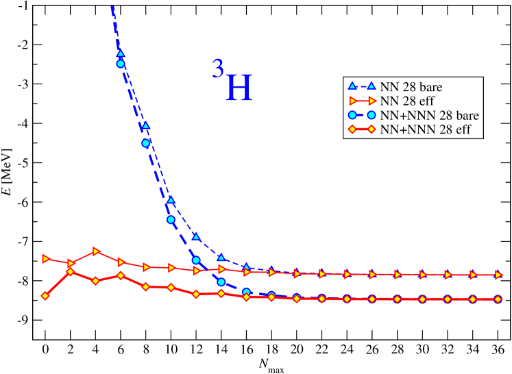
Figure 6: (Color online) ³H ground-state energy dependence on the size of the basis. The HO frequency of $\hbar\Omega=28$ MeV was employed. Results with (thick lines) and without (thin lines) the NNN interaction are shown. The full lines correspond to calculations with two-body effective interaction derived from the chiral NN interaction, the dashed lines to calculations with the bare chiral NN interaction. For further details see the text.

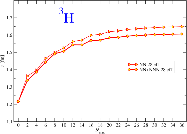
Figure 7: (Color online) ³H point-proton rms radius dependence on the size of the basis. The HO frequency of $\hbar\Omega=28$ MeV was employed. Results with (thick line) and without (thin line) the NNN interaction are shown. The two-body effective interaction derived from the chiral NN interaction was used in the calculation. For further details see the text.

In Figs. 8 and 9, we show convergence of the ⁴He ground-state energy and point-proton rms radius, respectively. The NCSM calculations are perforemed in basis spaces up to $N_{\rm max}=20$. Thin lines correspond to results obtained with the NN interaction only, while thick lines correspond to calculations that also include the NNN interaction. The dashed lines correspond to results obtained with bare interactions. The full lines correspond to results obtained using three-body effective interaction (the NCSM three-body cluster approximation). It is apparent that the use of the three-body effective interaction improves the convergence rate dramatically. We can see that at about $N_{\rm max}=18$ the bare interaction calculation reaches convergence as well. It should be noted, however, that $p$-shell calculations with the NNN interactions are presently feasible in model spaces up to $N_{\rm max}=6$ or $N_{\max}=8$. The use of the three-body effective interaction is then essential in the $p$-shell calculations.

Table 2: Ground-state energy and point-proton rms radius of ³H and ⁴He calculated using the chiral N³LO NN potential N3LO with and without the local chiral N²LO NNN interaction. The LECs values and other parameters are given in Table 1. The calculations were performed within the ab initio NCSM.

3H
	NN	NN+NNN	Expt.
$E_{\rm gs}$ [MeV]	-7.852(5)	-8.473(5)	-8.482
$r_{p}$ [fm]	1.650(5)	1.608(5)
4He
	NN	NN+NNN	Expt.
$E_{\rm gs}$ [MeV]	-25.39(1)	-28.34(2)	-28.296
$r_{p}$ [fm]	1.515(2)	1.475(2)	1.455(7)

Table 3: Contributions of different NNN terms to the ³H ground-state energy. The $c_{D}$ and $c_{E}$ LECs are explicitly shown. Other parameters are given in Table 1. All energies are given in MeV. The two alternative one-pion-exchange plus contact terms (50) and (51) are considered.

3H
$c_{D}$	$c_{E}$	$E_{\rm gs}$	$c$ terms	$D$ term	$E$ term
1.0 (Eq. (50))	-0.029	-8.473	-1.01	0.13	0.03
-1.0 (Eq. (50))	-0.331	-8.474	-1.07	-0.16	0.32
1.0 (Eq. (51))	-0.159	-8.471	-0.99	0.005	0.14
-1.0 (Eq. (51))	-0.213	-8.474	-1.10	-0.05	0.21

Figure 8: (Color online) ⁴He ground-state energy dependence on the size of the basis. The HO frequencies of $\hbar\Omega=28$ and 36 MeV was employed. Results with (thick lines) and without (thin lines) the NNN interaction are shown. The full lines correspond to calculations with three-body effective interaction, the dashed lines to calculations with the bare interaction. For further details see the text.

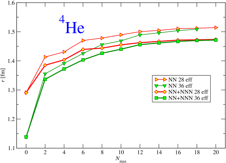
Figure 9: (Color online) ⁴He point-proton rms radius dependence on the size of the basis. The HO frequencies of $\hbar\Omega=28$ and 36 MeV was employed. Results with (thick line) and without (thin line) the NNN interaction are shown. The three-body effective interaction was used in the calculation. For further details see the text.

We note that NCSM calculations in the three-body cluster approximation are rather involved. The ⁴He NCSM calculation with the three-body effective interaction proceeds in three steps. First, we diagonalize the Hamiltonian with and without the NNN interaction in a three-nucleon basis for all relevant three-body channels. In the second step, we use the three-body solutions from the first step to derive three-body effective interactions with and without the NNN interaction. By subtracting the two effective interactions we isolate the NN and NNN contributions. This is needed due to a different scaling with particle number of the two- and the three-body interactions. The ⁴He efffective interaction is then obtained by adding the two contributions with the appropriate scaling factors NO03 . In the third step, we diagonalize the resulting Hamiltonian in the antisymmetrized four-nucleon Jacobi-coordinate HO basis to obtain the ⁴He $J^{\pi}T=0^{+}0$ ground state. Obviously, in calculations without the NNN interaction, the above three steps are simplified as no NNN contribution needs to be isolated. In addition, in the case of no NNN interaction, we may use just the two-body effective interaction (two-body cluster approximation), which is much simpler. The convergence is slower, however, see discussion in Ref. NO02 . We also note that ⁴He properties with the chiral N³LO NN interaction that we employ here were calculated using two-body cluster approximation in Ref. NC04 and present results are in agreement with results found there.

Our ⁴He results are summarized in Table 2. We note that the present NCSM ³H and ⁴He results obtained with the chiral N³LO NN interaction are in a perfect agreement with results obtained using the variational calculations in the hyperspherical harmonics basis as well as with the Faddeev-Yakubovsky calculations published in Ref. HHnonloc . A satisfying feature of the present NCSM calculation is the fact that the rate of convergence is not affected in any significant way by inclusion of the NNN interaction.

IV Conclusions

In this paper, we regulated the NNN interaction derived within the chiral effective field theory at the N²LO with a function depending on the magnitude of the momentum transfer. The regulated NNN interaction is local in the coordinate space. This is advantages for some many-body techniques. In addition, it was found that this interaction performs sligthtly better in mid-$p$-shell nuclei than its nonlocal counterpart Navratil:2007 ; Nogga_pc . We calculated matrix elements of the local chiral NNN interaction in the three-nucleon HO basis and performed calculations for ³H and ⁴He within the ab initio NCSM. We demonstrated that a very good convergence of the ground-state properties of these nuclei remains unchanged when the NNN interaction is added to the Hamiltonian. Expressions for the local $\chi$EFT NNN interaction matrix elements derived in this paper may by used after some modifications with other bases, e.g. with the hyperspherical harmonics basis.

References

• (1) S. Weinberg, Physica 96A, 327 (1979); Phys. Lett. B 251, 288 (1990); Nucl. Phys. B363, 3 (1991); J. Gasser et al., Ann. of Phys. 158, 142 (1984). Nucl. Phys. B250, 465 (1985).
• (2) V. Bernard, N. Kaiser, and Ulf-G. Meißner , Int. J. Mod. Phys. E4, 193 (1995).
• (3) C. Ordonez, L. Ray, and U. van Kolck, Phys. Rev. Lett. 72, 1982 (1994). Phys. Rev. C 53, 2086 (1996).
• (4) U. van Kolck, Prog. Part. Nucl. Phys. 43, 337 (1999).
• (5) P. F. Bedaque and U. van Kolck, Ann. Rev. Nucl. Part. Sci. 52, 339 (2002); E. Epelbaum, Prog. Part. Nucl. Phys. 57, 654 (2006).
• (6) S. R. Beane, P. F. Bedaque, K. Orginos, and M. J. Savage, Phys. Rev. Lett. 97, 012001 (2006).
• (7) S. R. Beane, P. F. Bedaque, M. J. Savage and U. van Kolck, Nucl. Phys. A700, 377 (2002); A. Nogga, R. G. Timmermans, and U. van Kolck, Phys. Rev. C 72, 054006 (2005).
• (8) M. C. Birse, Phys. Rev. C 74, 014003 (2006).
• (9) E. Epelbaum and U.-G. Meissner, nucl-th/0609037.
• (10) U. van Kolck, Phys. Rev. C 49, 2932 (1994).
• (11) E. Epelbaum, A. Nogga, W. Glöckle, H. Kamada, Ulf-G. Meissner and H. Witala, Phys. Rev. C 66, 064001 (2002).
• (12) E. Epelbaum, Phys. Lett. B 639, 456 (2006).
• (13) D. R. Entem and R. Machleidt, Phys. Rev. C 68, 041001(R) (2003).
• (14) P. Navrátil and V. G. Gueorguiev and J. P. Vary, W. E. Ormand and A. Nogga, Phys. Rev. Lett. 99, 042501 (2007); nucl-th/0701038.
• (15) P. Navrátil, J. P. Vary and B. R. Barrett, Phys. Rev. Lett. 84, 5728 (2000); Phys. Rev. C 62, 054311 (2000).
• (16) P. Navrátil and W. E. Ormand, Phys. Rev. C 68, 034305 (2003).
• (17) S. Quaglioni and P. Navrátil, Phys. Lett. B (2007), doi:10.1016/j.physletb.2007.06.082; arXiv:0704.1336.
• (18) A. Nogga, P. Navrátil, B. R.  Barrett and J. P.  Vary Phys. Rev. C 73, 064002 (2006).
• (19) B. S. Pudliner, V. R. Pandharipande, J. Carlson, and R. B. Wiringa, Phys. Rev. Lett. 74, 4396 (1995).
• (20) S. A. Coon, M. D. Scadron, P. C. McNamee, B. R. Barrett, D. W. E. Blatt and B. H. J. McKellar, Nucl. Phys. A 317, 242 (1979).
• (21) J. L. Friar, D. Hüber, and U. van Kolck, Phys. Rev. C 59, 53 (1999).
• (22) S. A. Coon and H. K. Han, Few-Body Systems 30, 131 (2001).
• (23) S. C. Pieper, Nucl. Phys. A571, 516 (2005).
• (24) S. C. Pieper, R. B. Wiringa and J. Carlson, Phys. Rev. C 70, 054325 (2004).
• (25) R. B. Wiringa, V. G. J. Stoks, and R. Schiavilla, Phys. Rev. C 51, 38 (1995).
• (26) S. C. Pieper, V. R. Pandharipande, R. B. Wiringa, and J. Carlson, Phys. Rev. C 64, 014001 (2001).
• (27) S. C. Pieper, K. Varga and R. B. Wiringa, Phys. Rev. C 66, 044310 (2002); R. B. Wiringa and S. C. Pieper, Phys. Rev. Lett. 89, 182501 (2002).
• (28) S. A. Coon and W. Glöckle, Phys. Rev. C 23 1790, (1981).
• (29) J. L. Friar, B. F. Gibson, G. L. Payne, and S. A. Coon, Few-Body Systems 5, 13 (1988).
• (30) S. A. Coon and M. T. Peña, Phys. Rev. C 48, 2559 (1993).
• (31) D. Hüber, H. Witala, A. Nogga, W. Glöckle, and H. Kamada, Few-Body Systems 22, 107 (1997).
• (32) D. Hüber, J. L. Friar, A. Nogga, H. Witala, and U. van Kolck, Few-Body Systems 30, 95 (2001).
• (33) N. Barnea, V. D. Efros, W. Leidemann, and G. Orlandini, Few-Body Systems 35, 155 (2004).
• (34) J. Adam, Jr., M. T. Peña, and A. Stadler, Phys. Rev. C 69, 034008 (2004).
• (35) P. Navrátil, G. P. Kamuntavičius, and B. R. Barrett, Phys. Rev. C 61, 044001 (2000).
• (36) D. C. J. Marsden, P. Navrátil, S. A. Coon and B. R. Barrett, Phys. Rev. C 66, 044007 (2002).
• (37) A. Nogga, private communication.
• (38) C. Hanhart, U. van Kolck, and G. A. Miller, Phys. Rev. Lett. 85, 2905 (2000).
• (39) P. Navrátil and W. E. Ormand, Phys. Rev. Lett. 88 (2002) 152502.
• (40) P. Navrátil and E. Caurier, Phys. Rev. C 69 (2004) 014311.
• (41) M. Viviani, L. E. Marcucci, S. Rosati, A. Kievsky and L. Girlanda, Few-Body Systems 39, 159 (2006).