Indication of multiscaling in the volatility return intervals of stock markets
Abstract
The distribution of the return intervals between price volatilities above a threshold height for financial records has been approximated by a scaling behavior. To explore how accurate is the scaling and therefore understand the underlined non-linear mechanism, we investigate intraday datasets of 500 stocks which consist of the Standard & Poor’s 500 index. We show that the cumulative distribution of return intervals has systematic deviations from scaling. We support this finding by studying the -th moment , which show a certain trend with the mean interval . We generate surrogate records using the Schreiber method, and find that their cumulative distributions almost collapse to a single curve and moments are almost constant for most range of . Those substantial differences suggest that non-linear correlations in the original volatility sequence account for the deviations from a single scaling law. We also find that the original and surrogate records exhibit slight tendencies for short and long , due to the discreteness and finite size effects of the records respectively. To avoid as possible those effects for testing the multiscaling behavior, we investigate the moments in the range , and find the exponent from the power law fitting has a narrow distribution around which depend on for the 500 stocks. The distribution of for the surrogate records are very narrow and centered around . This suggests that the return interval distribution exhibit multiscaling behavior due to the non-linear correlations in the original volatility.
pacs:
89.65.Gh, 05.45.Tp, 89.75.DaI Introduction
The price dynamics of financial markets has long been a focus of economics and econophysics research Mandelbrot63 ; Mantegna95 ; Kondor99 ; Mantegna00 ; Takayasu97 ; Liu99 ; Weber07 ; Bouchaud03 . Studying the volatility time series is not only crucial for revealing the underlined mechanism of financial markets dynamics, but also useful for traders. For example, it helps traders to estimate the risk and optimize the portfolio Bouchaud03 ; Johnson03 . The volatility series is known to be long-term power-law correlated Ding83 ; Wood85 ; Harris86 ; Admati88 ; Schwert89 ; Dacorogna93 ; Granger96 ; Pagan96 ; Liu97 ; Cizeau97 ; Cont98 ; Pasquini99 . To better understand these correlations and characterize temporal scaling features in volatilities, recently Yamasaki et al. Yamasaki05 and Wang et al. Wang06 ; Wang07 studied the statistics of return intervals between volatilities that are above a given threshold , which is an alternative way to analyze long-term correlated time series (see Ref Altmann05 and references therein). They find that scaling and memory in the return intervals of daily and intraday financial records are similar to that found in the climate and earthquake data Bunde04 ; Bunde05 ; Livina05 .
Studies of financial records show that the scaling in the return intervals distribution can be well approximated by a scaling function Yamasaki05 ; Wang06 ; Wang07 . However, financial time series are known to show complex behavior and are not of uniscaling nature Matteo07 and non-linear features Cao92 . Recent studies Ivanov04 ; Eisler06A ; Eisler06B of stock markets show that the distribution of activity measure such as the intertrade time has multiscaling behavior. Thus, a detailed analysis of the scaling properties of the volatility return intervals is of interest. It might improve our understanding of the return intervals statistics and shed light on the underlined complex mechanism of the volatility. Our analysis suggests that for all Standard & Poor’s index constituents, the cumulative distributions of the return intervals depart slightly but systematically from a single scaling law. We also find that the moments are consistent with the deviations from scaling. However, using the corresponding surrogate records Schreiber96 ; Makse96 ; Schreiber00 which remove the non-linearities, almost does not depend on and no deviation from scaling occur. Therefore, our results suggest that non-linear correlations in the volatility account for the deviations from a scaling law.
The paper is organized as follows: In section II we introduce the database and define the volatility. In section III we discuss the scaling and investigate the deviations from scaling in the cumulative distributions of the return intervals. We also describe the stretched exponential form suggested for the distribution and the generation of the surrogate records. Section IV deals with the moments of the return intervals. We quantify the deviation from the scaling that exhibits multiscaling behavior. We simulate the return intervals with different sizes and show the finite size effect for long . We also study the discreteness effect for short and explore the relation between the moment and its order. In Section V we present a discussion.
II Database
We analyze the Trades And Quotes (TAQ) database from New York Stock Exchange (NYSE), which records every trade for all the securities in United States stock markets. The duration is from Jan 1, 2001 to Dec 31, 2002, which has a total of 500 trading days. We study all 500 companies which consist of the Standard & Poor’s 500 index (S&P 500) Note1 , the benchmark for American stock markets. The volatility is defined the same as in Wang06 . First we take the absolute value for the logarithmic price change, then remove the intraday U-shape pattern, and finally normalize it with the standard deviation. Here the price is the closest tick to a minute mark. Thus the sampling time is 1 minute and a trading day usually has 391 points after removing the market closing hours. For each stock, the size of dataset is about 200,000 records.
III Scaling in Return Intervals
The probability density function (PDF) for the return intervals of the financial volatilities is well-approximated by the following form,
| (1) |
as analyzed by Yamasaki et al. Yamasaki05 and Wang et al. Wang06 ; Wang07 . Here stands for the average over the dataset and depends on the threshold . It was suggested that the scaling function can be approximated by a stretched exponential Yamasaki05 ; Wang06 ; Wang07 ,
| (2) |
for financial records, which is consistent with other long-term correlated records Altmann05 ; Bunde04 ; Bunde05 ; Livina05 . Here and are fitting parameters and is the exponent characterizing the long-term correlation Altmann05 ; Bunde04 ; Bunde05 ; Livina05 . From the normalization of PDF follows Note2 ,
| (3) |
From the definition of follows,
| (4) |
Thus, using Eqs. (3) and (4), the parameters and can be expressed by ,
| (5) |
Here is the Gamma function. Thus, if the stretched exponential distribution is valid for the scaled interval , it is completely determined by . For , the record has no long-term correlations and the return interval distribution indeed follows an exponential distribution, represented by a Poissonian statistics, as expected.
Though the scaling in the return intervals distribution is a good approximation, we find slight deviations that as shown below are attributed to non-linear features. To explicitly explore the quality of the scaling in return interval distributions, we study all S&P 500 constituents and show the results of four representative stocks, Citigroup (C), General Electric (GE), Coca Cola (KO) and Exxon Mobil (XOM). All other stocks studied here usually show similar features. First, we examine the cumulative distribution of the scaled intervals.
| (6) |
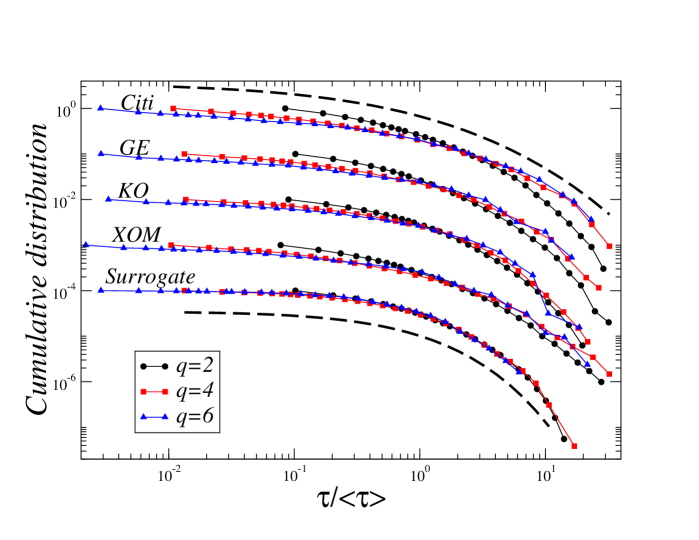
If the scaling function is valid, the cumulative distributions should also collapse to a single curve. Otherwise, the cumulative distributions, which integrate deviations, may show clearer deviations from scaling. Indeed, in Fig. 1 we show cumulative distributions for three thresholds , and . Note that the volatility is normalized by its standard deviation, the threshold is in units of standard deviations and therefore is a quite large volatility. It is clearly seen that those distributions are close to each other but do not collapse to a single curve. More important, they show apparent deviations from the scaling, which are systematic with the threshold. For small scaled intervals (), the cumulative distribution decreases with , while for large scaled intervals (), it increases with Note3 . In other words, the scaled interval prefers to be larger for higher threshold. This systematic trend suggests multiscaling in the return intervals, which might be related to the non-linear correlations in the volatility.
To better understand the systematic trends and test if it is not due to finite size effect or discreteness of minutes, we also measure the cumulative distribution of return intervals for surrogate records of volatilities using the Schreiber method Schreiber96 ; Makse96 ; Schreiber00 where non-linearities are removed. For a given time series, we store the power spectrum and randomly shuffle the sequence, then we apply the following iterations. Each iteration consists of two consecutive steps:
(i) We perform the Fourier transform of the shuffled series, replace its power spectrum with the original one, then take the inverse Fourier transform to achieve a series. This step enforces the desired power spectrum to the series, while the distribution of volatilities usually is modified.
(ii) By ranking, we exchange the values of the resulting series from step (i) with that of the original record. The largest value in the resulting series is replaced by the largest one in the original series, the second largest value is replaced by the second largest one, and so on. This step restores the original distribution but now the power spectrum is changed.
To achieve the convergence to the desired power spectrum and distribution, we repeat these two steps 30 times. By this way, a “surrogate” series is generated. Because of the Wiener-Kinchine theorem Kampen92 , the surrogate record has the same linear correlations as the original, as well as the distribution. The only difference is that the original record has the non-linear correlations (if they exist) but the surrogate does not have any non-linear features.
In Fig. 1 we also plot the cumulative distribution for the surrogate with the same three thresholds as the original. Since the surrogate records lost the non-linear correlations, they are similar to each other, we only show results for GE’s surrogate. It is seen that the collapse of the surrogate for different values is significantly better than that of the original and the deviation tendency with the threshold in the original records disappears. This indicates that the scaling deviations in the original are due to the non-linear correlations in the volatility. To further test this hypothesis, we analyze the moments in Sec. (IV) and show similar and consistent deviations from scaling. We also compare our results to the stretched exponential distribution (dashed lines). This curve is very close to the empirical results, in particular for the surrogate records which contain only the linear correlations. This suggests that PDF of return intervals is well approximated by a stretched exponential.
IV The Moments of Scaled Intervals
The cumulative distribution shows clear systematic trend with , which is difficult to see from the PDF directly Yamasaki05 ; Wang06 ; Wang07 ; Altmann05 ; Bunde04 ; Bunde05 . To further analyze the systematic tendency in the distribution, we calculate the moments averaged over a stock dataset as a function of , where a mean interval corresponds to a threshold and therefore characterizes a return interval series. We study moments for a wide range of , from minutes (to avoid the artificial effects due to discreteness close to ) to thousands minutes (few trading days or even a week). Assuming a single scaling function for the PDF , Eq. (1), it follows
| (7) |
which only depends on and on the form of the scaling function but independent of . Thus, if depends on , it suggests deviation from the assumption of scaling.
IV.1 Moments vs. Mean Interval
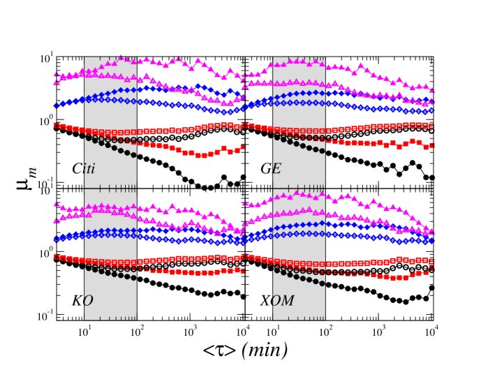
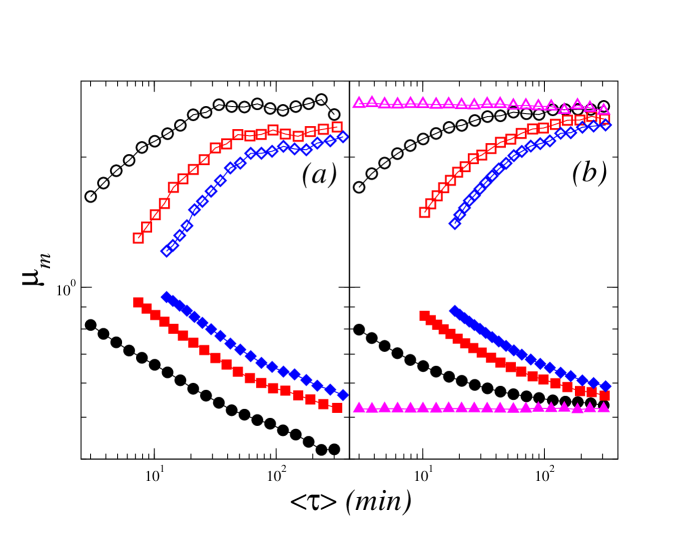
First we examine the relation between the moments and the mean interval . Fig. 2 shows four representative moments , , and for stock C, GE, KO and XOM. Ignoring small fluctuations, which is usually due to limited size data, all moments for the original records deviate significantly from a horizontal line, which is expected for a perfect scaling of the PDF. They depend on and show some systematic tendency. For , moments have similar convex structure, first increases with and then decreases, where the crossover starts earlier for larger . For , moments also show similar tendency but in the opposite direction compared to . These deviations from scaling in are consistent with the deviations seen in the cumulative distributions shown in Fig. 1. Moments of large () represent large in the PDF and they initially (for ) increase with , while moments of small () represent small and they initially (for ) decrease with .
To further test if the systematic deviations are not due to finite size effects and discreteness, we also examine moments for the surrogate records which are more flat for most range, as shown in Fig. 2. For the same order , the moment of the surrogate obviously differs from that of the original, especially in the medium range of (). This discrepancy suggests that the non-linear correlations exist in the original volatility and accounts for the scaling deviations. Nevertheless, all moments of surrogate show small curvature from a perfect straight line at both short and long , which are much weaker compared to the original records. The weak curvature suggests that some additional effects, not related to the non-linear correlations, affect the moments. For small , the resolution discrete limit seems to have some influence on the moments. We will discuss this effect in section C. For large , the moments are gradually approaching the horizontal line and are more fluctuating, the effect seems to be related to limited size of the record. This effect will be discussed in section B.
IV.2 Multiscaling
For the original volatility records, the systematic tendency in the distribution of and the moments implies that the return intervals may have multiscaling features. To avoid as much as possible the effect of discreteness and finite size, we calculate the moments only for some medium range of where the effects are small. Since there is no non-linear correlations in the surrogate records, the curvature in their moments is only due to the additional effects, we use the surrogate curve as our reference. For small , the increasing (decreasing) range for () almost ends at minutes. For large , the curves start to decrease (increase) from different positions, but at , all curves do not or just start to decrease (increase). Thus we choose to study in the region, , represented by the shadow areas in Fig. 2. In this range, we find a clear trend for the original records while the surrogate is almost horizontal. To quantify the tendency, we fit the moments with a power-law,
| (8) |
If the distribution of follows a scaling law, the exponent should be some value very close to . If is significantly different from , it suggests multiscaling.
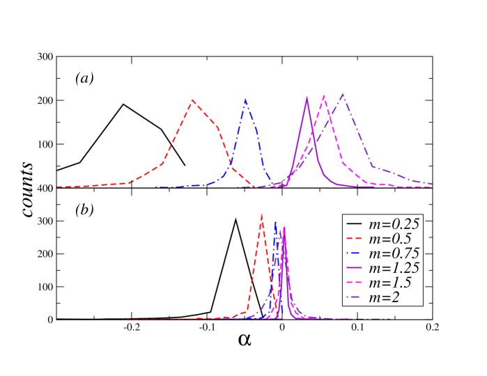
To examine the multiscaling behavior for the whole market, we calculate for all 500 stocks of S&P 500 constituents and plot the histogram for to . Fig. 3 shows that each histogram has a narrow distribution, which suggests that are similar for the 500 stocks. For the original records, almost all significantly differ from , thus the moments clearly depend on the mean interval. Moreover, the mean value of shifts with order from for to for which means the dependence varies with the order . This behavior suggests multiscaling in the return intervals distribution. Indeed, histograms for the surrogate records are more centered around values close to . The uniscaling behavior for the surrogate suggests that the non-linear correlations in the volatility are responsible for the multiscaling behavior in the original.
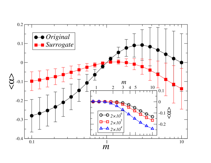
To remove fluctuations and show the tendency clearer, we plot the dependence of on , where is the average over all 500 stocks. In Fig. 4 we show this relation for a wide range of , , and the plot shows two different behaviors. For small (roughly ), for the original records clearly deviates from 0 and demonstrates the multiscaling behavior, while for the surrogate is closer to . For large (), the two curves have similar decreasing trend. Since large dominates high order moments, this similarity may be due to finite size effects. To test the finite size effects we simulate surrogate return intervals by assuming a stretched exponential distribution i.i.d. process with 3 sizes (number of all in the series), , (the size of the empirical dataset) and . Without loss of generality, we choose , which is the correlation exponent for GE of . To be consistent with the 500 stocks, we perform 500 realizations and plot their average exponent . As shown in the inset of Fig. 4, all show a similar decreasing trend as that of the empirical curves. However, it is seen that the trend starts earlier for smaller size, and thus the size limit has a strong influence on high order moments. Fig. 4 also shows the error bars for the two records, which is the standard deviation of 500 values. Note that the error bars for the volatility records do not overlap those of their corresponding surrogate, indicating the significance of our results.
IV.3 Discreteness Effect
For small (), the behavior of as a function of was attributed to the discreteness. Here we examine this effect. Due to the limits in recording, we can not have a continuous but discrete record. In our study the volatility is recorded in 1 minute. The relative errors in moments will be considerable large for small close to minute. By starting from , we only partially avoid the discreteness in the moments. To test the discreteness effects, since we can not increase the resolution, we reduce it and compare the moments with 3 resolutions, 1 minute, 5 minutes and 10 minutes. Fig. 5(a) shows this comparison for GE for and . The three resolutions have a similar trend, showing that the curves become flatter for the higher resolution. For other stocks, we find similar behavior. This systematic tendency suggests that the recording limit (1 minute) strongly affects the moments at short . To reduce it, we should raise the recording precision or study the moments of larger .
To further test this result, we simulate artificial return intervals with an i.i.d. process from stretched exponential distribution with , same as the empirical for GE of . We examine moments of and with the same three resolutions (1, 5 and 10 time units) as in the empirical test done above. The simulated size is 200 thousands points for each trial and we use the average over 100 trials for each resolution. Fig. 5(b) shows curves similar to that of empirical (Fig. 5(a)). For the higher resolution, the curve is closer to the horizontal line and finally may reach the line when we raise the resolution high enough. To show this, we also simulate continuous return intervals and find constant moments, as expected (Fig. 5(b)). Therefore, the discreteness effects can be overcome if the resolution is improved enough. Note that for the empirical data, we expect the moment not to be constant for small even if we have a much better resolution, since the return intervals has the multiscaling behavior, as shown for larger in the range which is not affected by discreteness.
IV.4 Moments vs. Order
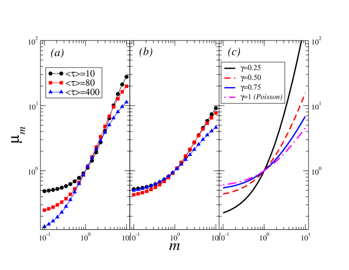
The moments have systematic dependence on , as seen in Figs. 2 and 3 where the moments are plotted as the function of . It is of interest to explore the relation between the moments and directly. For a fixed , representing a given threshold one can study, the return intervals and their moments of various orders which exhibit information on different scales of . Moments of large represent large and vice versa. If follows a single distribution without corrections due to effects such as discreteness and finite size, curves of vs. for different should collapse to a single one, which only depends on the scaling function from Eq. (7). In Fig. 6 we plot vs. for both the original and surrogate records. We plot for between and for three values: 10, 80 and 400 minutes. For the original (Fig. 6(a)), there is substantial deviations from a single curve. This supports our suggestion that the return intervals has multiscaling behavior. Moments for the surrogate (Fig. 6(b)) converge to a single curve for but become diverse for high orders, which agrees with the strong influence of the finite size effects. As a reference, we also plot the analytical moments (Fig. 6(c)) from the stretched exponential distribution. Substituting Eq. (2) into Eq. (7), we obtain
| (9) |
Fig. 6(c) shows analytical curves for various correlation exponent .
V Discussion
We study the scaling properties of the distribution of the volatility return intervals for all S&P 500 constituents. We find small but systematic deviations from scaling assumption with the threshold in the cumulative distribution. Compared to the good collapse for the surrogate records where non-linearities are removed, this suggests that the origin of this trend is due to non-linear correlations in the original volatility. Moreover, we find similar systematic deviations for the moments , which are also attributed to the non-linear correlations in the volatility. We distinguish these deviations from the deviations due to the discreteness for small and finite size effect for large . Further, we explore the dependence of the moment on its order . When compare to surrogate records and to analytical curves, the results support the multiscaling hypothesis of the return intervals. Thus, the scaling assumption in the return interval distributions although it is a good approximation can not be exact. Also, the stretched exponential form of the scaling function can only be an approximation. Recently Eisler et al. Eisler06A ; Eisler06B exhibits that the distribution of intertrade times has similar multiscaling behavior and the market activity depends on the company capitalization. It would be interesting to connect the intertrade times with the return intervals and test size dependence in the return intervals.
Acknowledgments
We thank Y. Ashkenazy for his kind help in the simulations, R. Mantegna, J. Kertész and Z. Eisler for fruitful discussions, and the NSF and Merck Foundation for financial support.
References
- (1) B. B. Mandelbrot, J. Business 36, 394 (1963).
- (2) R. N. Mantegna and H. E. Stanley, Nature (London) 376, 46 (1995).
- (3) Econophysics: An Emerging Science, edited by I. Kondor and J. Kertész (Kluwer, Dordrecht, 1999).
- (4) R. Mantegna and H. E. Stanley, Introduction to Econophysics: Correlations and Complexity in Finance (Cambridge Univ. Press, Cambridge, England, 2000).
- (5) H. Takayasu, H. Miura, T. Hirabayashi, and K. Hamada, Physica A 184, 127 (1992); H. Takayasu, A. H. Sato, and M. Takayasu, Phys. Rev. Lett. 79, 966 (1997); H. Takayasu and K. Okuyama, Fractals 6, 67 (1998).
- (6) Y. Liu, P. Gopikrishnan, P. Cizeau, M. Meyer, C.-K. Peng, and H. E. Stanley, Phys. Rev. E 60, 1390 (1999); V. Plerou, P. Gopikrishnan, X. Gabaix, L. A. Nunes Amaral, and H. E. Stanley, Quant. Finance 1, 262 (2001); V. Plerou, P. Gopikrishnan, and H. E. Stanley, Phys. Rev. E 71 , 046131 (2005).
- (7) P. Weber, F. Wang, I. Vodenska-Chitkushev, S. Havlin and H. E. Stanley, Phys. Rev. E 76, 016109 (2007).
- (8) J.-P Bouchaud and M. Potters, Theory of Financial Risk and Derivative Pricing: From Statistical Physics to Risk Management (Cambridge Univ. Press, Cambridge, 2003).
- (9) N. F. Johnson, P. Jefferies, and P. M. Hui, Financial Market Complexity (Oxford Univ. Press, New York, 2003).
- (10) Z. Ding, C. W. J. Granger and R. F. Engle, J. Empirical Finance 1, 83 (1983).
- (11) R. A. Wood, T. H. McInish, and J. K. Ord, J. Finance 40, 723 (1985).
- (12) L. Harris, J. Financ. Econ. 16, 99 (1986).
- (13) A. Admati and P. Pfleiderer, Rev. Financ. Stud. 1, 3 (1988).
- (14) G. W. Schwert, J. Finance 44, 1115 (1989); K. Chan, K. C. Chan, and G. A. Karolyi, Rev. Financ. Stud. 4, 657 (1991); T. Bollerslev, R. Y. Chou, and K. F. Kroner, J. Econometr. 52, 5 (1992); A. R. Gallant, P. E. Rossi, and G. Tauchen, Rev. Financ. Stud. 5, 199 (1992); B. Le Baron, J. Business 65, 199 (1992).
- (15) M. M. Dacorogna, U. A. Muller, R. J. Nagler, R. B. Olsen, and O. V. Pictet, J. Int. Money Finance 12, 413 (1993).
- (16) A. Pagan, J. Empirical Finance 3, 15 (1996).
- (17) C. W. J. Granger and Z. Ding, J. Econometr. 73, 61 (1996).
- (18) Y. Liu, P. Cizeau, M. Meyer, C.-K. Peng, and H. E. Stanley, Physica A 245, 437 (1997).
- (19) R. Cont, Ph.D. thesis, Universite de Paris XI, 1998 (unpublished); see also e-print cond-mat/9705075.
- (20) P. Cizeau, Y. Liu, M. Meyer, C.-K. Peng, and H. E. Stanley, Physica A 245, 441 (1997).
- (21) M. Pasquini and M. Serva, Econ. Lett. 65, 275 (1999).
- (22) K. Yamasaki, L. Muchnik, S. Havlin, A. Bunde, and H. E. Stanley, Proc. Natl. Acad. Sci. U.S.A. 102, 9424 (2005).
- (23) F. Wang, K. Yamasaki, S. Havlin, and H. E. Stanley, Phys. Rev. E 73, 026117 (2006).
- (24) F. Wang, P. Weber, K. Yamasaki, S. Havlin, and H. E. Stanley, Eur. Phys. J. B [Proc. Special Issue on Econophysics] 55, 123 (2007).
- (25) E. G. Altmann and H. Kantz, Phys. Rev. E 71, 056106 (2005).
- (26) A. Bunde, J. F. Eichner, S. Havlin, and J. W. Kantelhardt, Physica A 342, 308 (2004).
- (27) A. Bunde, J. F. Eichner, J. W. Kantelhardt, and S. Havlin, Phys. Rev. Lett. 94, 048701 (2005).
- (28) V. N. Livina, S. Havlin, and A. Bunde, Phys. Rev. Lett. 95, 208501 (2005).
- (29) T. Di Matteo, Quant. Finan. 7, 21 (2007).
- (30) C. Q. Cao and R. S. Tsay, J. Appl. Econometrics 7, S165 (1992).
- (31) P. Ch. Ivanov, A. Yuen, B. Podobnik, and Y. Lee, Phys. Rev. E 69, 056107 (2004).
- (32) Z. Eisler and J. Kertész, Phys. Rev. E 73, 046109 (2006).
- (33) Z. Eisler and J. Kertész, Eur. Phys. J. B 51, 145 (2006).
- (34) T. Schreiber and A. Schmitz, Phys. Rev. Lett. 77, 635 (1996).
- (35) H. A. Makse, S. Havlin, M. Schwartz, and H. E. Stanley, Phys. Rev. E 53, 5445 (1996).
- (36) T. Schreiber and A. Schmitz, Physica D 142, 346 (2000).
- (37) Note that S&P 500 constituents changes a small fraction every year. To fix datasets, we choose 500 stocks which has the longest time in the index for year 2001 and 2002.
- (38) Here we assume that the scaled interval is continuous. This assumption is not precisely accurate since the return intervals are discrete. However, the minimum scaled interval usually is not very large. For example, for GE return interval of , the corresponding minimum is
- (39) Note that for very large scaled intervals, , the curves have apparent fluctuations, which can not be trusted as much as that of smaller scaled intervals, due to poor statistics.
- (40) N. G. Van Kampen, Stochastic Processes in Physics and Chemistry (Revised and Enlarged Edition) (North-Holland, Amsterdam, 1992).
