Thermal conductivity of ions in a neutron star envelope

Abstract

We analyze the thermal conductivity of ions (equivalent to the conductivity of phonons in crystalline matter) in a neutron star envelope.

We calculate the ion/phonon thermal conductivity in a crystal of atomic nuclei using variational formalism and performing momentum-space integration by Monte Carlo method. We take into account phonon-phonon and phonon-electron scattering mechanisms and show that phonon-electron scattering dominates at not too low densities. We extract the ion thermal conductivity in ion liquid or gas from literature.

Numerical values of the ion/phonon conductivity are approximated by analytical expressions, valid for $T\ga 10^{5}\;{\rm K}$ and $10^{5}\leavevmode\nobreak\ {\rm g\leavevmode\nobreak\ cm^{-3}}\la\rho\la 10^{14}\leavevmode\nobreak\ {\rm g\leavevmode\nobreak\ cm^{-3}}$. Typical magnetic fields $B\sim 10^{12}$ G in neutron star envelopes do not affect this conductivity although they strongly reduce the electron thermal conductivity across the magnetic field. The ion thermal conductivity remains much smaller than the electron conductivity along the magnetic field. However, in the outer neutron star envelope it can be larger than the electron conductivity across the field, that is important for heat transport across magnetic field lines in cooling neutron stars. The ion conductivity can greatly reduce the anisotropy of heat conduction in outer envelopes of magnetized neutron stars.

1 Introduction

Neutron stars with strong magnetic fields $B\ga 10^{12}\;$G are expected to have an anisotropic surface temperature distribution (see, e.g., Gepert, Kueker & Page Geppert et al.2004, Geppert et al.2006, Pérez-Azorín et al.2006). It is thought to result from the anisotropy of thermal conduction in a neutron star envelope and manifests in periodic modulation of X-ray emission observed from some spinning neutron stars (e.g., Burwitz et al. 2003; Haberl 2007; Ho 2007). The thermal conductivity $\kappa_{\perp}$ across the magnetic field can be much smaller than the conductivity $\kappa_{\parallel}$ along the field (see, e.g., Yakovlev & Kaminker 1994; Potekhin 1999). Both conductivities are crucial for modeling of cooling magnetized neutron stars (Geppert et al.2006, Pérez-Azorín et al.2006, Page, Geppert & Weber Page et al.2006, and references therein).

In a non-magnetized envelope, thermal energy is mainly transported by electrons ($\kappa\approx\kappa_{\rm e}$; Flowers & Itoh 1976; Potekhin et al. 1999). The thermal conductivity of ions, $\kappa_{\rm i}$, in which we include the ion conductivity of an ion gas or liquid and the phonon conductivity of a crystalline ion solid, is usually much smaller than $\kappa_{\rm e}$. However, a strong enough magnetic field $B$ can easily suppress $\kappa_{{\rm e}\perp}$, making $\kappa_{\rm i}$ the leading thermal conductivity across the magnetic field (e.g., Pérez-Azorín et al.2006).

In this paper we analyze different regimes of the ion thermal conductivity in a neutron star envelope. Physical conditions in the envelope are described in Sect. 2. The thermal conductivity in the magnetized envelope is outlined in Sect. 3, where we give a sketch of anisotropic electron heat conduction and nearly isotropic ion/phonon heat transport. The ion conductivity due to ion-ion (phonon-phonon) scattering is studied in Sect. 4. The ion conductivity owing to ion-electron (phonon-electron) scattering is analyzed in Sect. 5. In Sect. 6 we estimate the values of magnetic fields which can strongly affect ion heat transport. Section 7 contains a discussion of our results. Conclusion is presented in Sect. 8.

2 Coulomb plasma in a neutron star envelope

We consider a model of a neutron star envelope which combines several models of ground state matter (Negele & Vautherin 1973; Oyamatsu 1993 and others) and which is summarized by Haensel, Potekhin & Yakovlev Haensel et al.2007 (their Appendix B). Typical densities and temperatures of practical interest are indicated in Fig. 1 and outlined below in this section. The shaded regions I–V are domains, where the ion thermal conductivity has different character. These domains are summarized in Table 1 and described further in Sects. 3–5. The last column of Table 1 gives the leading ion (phonon) scattering mechanism. In addition, in Fig. 1 we show the boundaries of the regions, where ion heat transport is strongly affected by the magnetic fields $B_{\mathrm{m}}=10^{13}$ G and $10^{14}$ G (the regions below and to the left of the lines).

At any density $\rho$ the plasma is assumed to consist of electrons and single species of fully ionized atoms (bare atomic nuclei). In the inner neutron star envelope, at densities higher the neutron drip density $\rho_{\mathrm{ND}}\approx 4.3\times 10^{11}$ g cm^-3 [shown by the vertical dot-dashed line in Fig. 1; Negele & Vautherin 1973] the matter contains also free neutrons.

We describe the parameters of dense matter following §2.1 in (Haensel et al.2007). The charge neutrality of the matter implies

$$n_{\mathrm{i}}=n_{\mathrm{e}}/Z\leavevmode\nobreak\ ,$$ (1)

where $Z$ is the charge number of the nuclei, while $n_{\mathrm{e}}$ and $n_{\mathrm{i}}$ are the electron and ion number densities, respectively. The mass density of the matter can be estimated as

$$\rho\approx n_{\mathrm{i}}A^{\prime}m_{\mathrm{u}}\leavevmode\nobreak\ ,$$ (2)

where $m_{\mathrm{u}}$ is the atomic mass unit and $A^{\prime}$ is the number of nucleons per one nucleus. For $\rho<\rho_{\mathrm{ND}}$, one has $A^{\prime}=A$, where $A$ is the number of nucleons confined in one nucleus. For $\rho>\rho_{\mathrm{ND}}$, one has $A^{\prime}=A+A^{\prime\prime}$, where $A^{\prime\prime}$ is the number of free (unbound) neutrons per one nucleus. The ion mass is

$$m_{\mathrm{i}}=A\,m_{\mathrm{u}}.$$ (3)

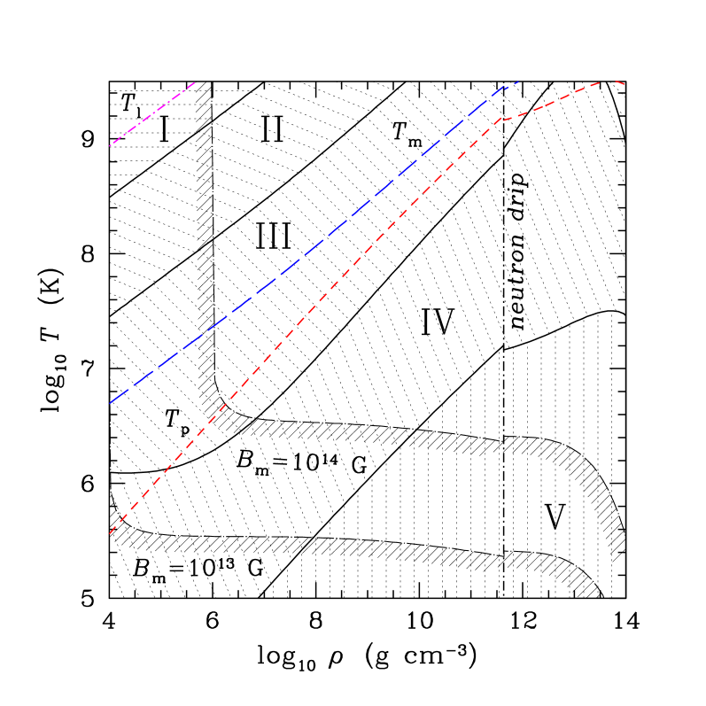
Figure 1: (color online) Temperature-density diagram for the ground-state neutron star crust (smooth-composition model, Haensel et al.2007); $T_{\mathrm{l}}$ is the temperature for the onset of Coulomb coupling of ions into ion liquid; $T_{\mathrm{m}}$ is the crystallization temperature of ions; $T_{\mathrm{p}}$ is the ion plasma temperature; the vertical line shows the neutron drip density. Shaded are regions I–V of different regimes (Table 1) of the ion thermal conductivity. Also, we show the boundaries of the regions where ion heat transport can be strongly affected by the magnetic fields $B_{\mathrm{m}}=10^{13}$ G and $10^{14}$ G. See text for details.

Table 1: Ion conduction regimes I–V in Fig. 1.

Regime	State of ions	Leading
		scattering∗
I	Weakly coupled ions	ii
II	Classical ion liquid	ii
III	Low-$T$ liquid, high-$T$ crystal	ii (ph ph)
IV	Quantum ion crystal	ie (ph e)
V	Very cold quantum crystal	ie (ph e) and
		possibly others

^∗Symbols i, e, and ph refer to ions, electrons, and phonons, respectively.

First, we describe the properties of electrons (Sect. 2.1) and ions (Sect. 2.2) neglecting the effects of the magnetic fields, and then (Sect. 3) we outline the magnetic effects.

2.1 Electrons

Under the conditions of study (Fig. 1), the electrons are typically strongly degenerate. The electron Fermi momentum $p_{\mathrm{F}}$ and Fermi wavenumber $k_{\mathrm{F}}$ are

$$p_{\mathrm{F}}=\hbar k_{\mathrm{F}}=\hbar\,(3\pi^{2}n_{\mathrm{e}})^{1/3}\leavevmode\nobreak\ .$$ (4)

The electron relativity parameter can be written as

$$x_{\mathrm{r}}={p_{\mathrm{F}}\over m_{\mathrm{e}}c}\approx 1.009\left({\rho_{6}Z\over A^{\prime}}\right)^{1/3}\leavevmode\nobreak\ \;,$$ (5)

where $\rho_{6}\equiv\rho/10^{6}\leavevmode\nobreak\ {\rm g\leavevmode\nobreak\ cm^{-3}}$. The electron Fermi energy and the effective mass at the Fermi surface take the form

$$\epsilon_{\mathrm{F}}=m_{\mathrm{e}}c^{2}(1+x_{\mathrm{r}}^{2})^{1/2}\;,\leavevmode\nobreak\ \leavevmode\nobreak\ m_{\mathrm{e}}^{\ast}=m_{\mathrm{e}}\left(1+x_{\mathrm{r}}^{2}\right)^{1/2}={\epsilon_{\mathrm{F}}\over c^{2}}\leavevmode\nobreak\ ,$$ (6)

and the electron Fermi velocity reads

$$v_{\mathrm{F}}={p_{\mathrm{F}}\over m^{\ast}_{\mathrm{e}}}=c\,{x_{\mathrm{r}}\over\left(1+x_{\mathrm{r}}^{2}\right)^{1/2}}\leavevmode\nobreak\ .$$ (7)

The electron degeneracy temperature is

$$T_{\mathrm{F}}={\epsilon_{\mathrm{F}}-m_{\mathrm{e}}c^{2}\over k_{\mathrm{B}}}=5.93\times 10^{9}\left[\sqrt{1+x_{\mathrm{r}}^{2}}-1\right]\;{\rm K}\;,$$ (8)

where $k_{\mathrm{B}}$ is the Boltzmann constant. The electrons are strongly degenerate as long as $T\ll T_{\mathrm{F}}$.

Finally, the electron Thomas-Fermi screening wavenumber (inverse plasma screening length of Coulomb interaction due to polarizability of strongly degenerate electrons) is

$$k_{\mathrm{TF}}=2\left(\alpha\;c\over\pi v_{\mathrm{F}}\right)^{1/2}k_{\mathrm{F}}\leavevmode\nobreak\ ,$$ (9)

where $\alpha$ is the fine structure constant.

2.2 Ions

The properties of the classical ion plasma are determined by the Coulomb coupling parameter

$$\Gamma={Z^{2}e^{2}\over a_{\mathrm{i}}k_{\mathrm{B}}T}\leavevmode\nobreak\ ,$$ (10)

where

$$a_{\mathrm{i}}=\left(4\pi n_{\mathrm{i}}/3\right)^{-1/3}\leavevmode\nobreak\$$ (11)

is the ion sphere radius. The plasma ions form a nearly ideal gas as long as $\Gamma\ll 1$ which corresponds to $T\gg T_{\mathrm{l}}=Z^{2}e^{2}/(a_{\mathrm{i}}k_{\mathrm{B}})$. At lower $T$ they transform smoothly into a strongly coupled ion liquid.

It is also important to define the ion plasma frequency

$$\omega_{\mathrm{p}}=\left(4\pi n_{\mathrm{i}}Z^{2}\,e^{2}/m_{\mathrm{i}}\right)^{1/2}\leavevmode\nobreak\ ,$$ (12)

and the associated ion plasma temperature

$$T_{\mathrm{p}}={\hbar\omega_{\mathrm{p}}\over k_{\mathrm{B}}}=7.832\times 10^{6}\;\left({\rho_{6}\over A^{\prime}}\;{Z^{2}\over A}\right)^{1/2}\;{\rm K}\leavevmode\nobreak\ ,$$ (13)

displayed in Fig. 1. Quantum effects in ion motion become very important for $T\ll T_{\mathrm{p}}$.

The conditions of ion crystallization are described, e.g., in (Haensel et al.2007), §2.3.4. A classical Coulomb liquid of ions crystallizes at the temperature

$$T_{\mathrm{m}}={Z^{2}e^{2}\over a_{\mathrm{i}}k_{\mathrm{B}}\Gamma_{\mathrm{m}}}\approx 1.3\times 10^{5}\;Z^{2}\left({\rho_{6}\over A^{\prime}}\right)^{1/3}\;{175\over\Gamma_{\mathrm{m}}}\;{\rm K}\leavevmode\nobreak\ ,$$ (14)

where $\Gamma_{\mathrm{m}}\approx 175$. Large zero-point vibrations of ions at very high densities can reduce $T_{\mathrm{m}}$ or even prevent crystallization. Actually, this effect can be important only for a plasma of light nuclei (hydrogen and helium) which we do not consider here. Ions are usually assumed to form body-centered cubic lattice, but, in fact, the face centered cubic lattice is also possible (see, e.g., Baiko 2002). We study phonon conductivities for both lattice types and find, that they are nearly identical. The same is true for other kinetic and thermodynamic properties of such crystals (see, e.g., Baiko et al. 1998, 2001).

3 Thermal conductivity in a magnetized plasma

As outlined in Sect. 1, we are interested in the thermal conductivity of magnetized neutron star envelopes. A magnetic field $\bm{B}$ makes thermal conduction anisotropic (e.g., Yakovlev & Kaminker 1994; Potekhin 1999). The total thermal conductivity can be written as

$$\kappa=\kappa_{\mathrm{e}}+\kappa_{\mathrm{i}},$$ (15)

where $\kappa_{\mathrm{e}}$ and $\kappa_{\mathrm{i}}$ are the conductivities of electrons and ions, respectively. In the inner envelope of a neutron star one should also add the thermal conductivity of neutrons. However, it is largely unexplored and will be neglected here. Generally, both conductivities, $\kappa_{\mathrm{e}}$ and $\kappa_{\mathrm{i}}$, are anisotropic tensor quantities. Nevertheless, a typical neutron star magnetic field $B\sim 10^{12}-10^{13}$ G can strongly affect the electron thermal conduction (see, e.g., Yakovlev & Kaminker 1994; Potekhin 1999) but weakly affects the ion thermal conduction (see Sec. 6). Therefore, we will take into account the effect of the magnetic field on $\kappa_{\mathrm{e}}$ but neglect its effect on $\kappa_{\mathrm{i}}$. Let us emphasize that our aim is to study the ion conductivity. We describe the electron conductivity here only for comparison with the ion one.

3.1 Thermal conductivity of electrons

An anisotropic electron conduction in a magnetic field $\bm{B}$ is characterized by the thermal conductivity $\kappa_{\mathrm{e\parallel}}$ along the magnetic field, by the conductivity $\kappa_{\mathrm{e\perp}}$ across the field, and by the Hall conductivity $\kappa_{\mathrm{eH}}$ (perpendicular to $\bm{B}$ and to the temperature gradient). The effects of the magnetic fields on electron thermal conduction are twofold (see, e.g., Yakovlev & Kaminker 1994; Ventura & Potekhin 2001).

First, there are classical effects associated with electron Larmor rotation about magnetic field lines. Their efficiency is characterized by the electron magnetization parameter $\omega_{\mathrm{g}}\tau_{\mathrm{e}}$ (see e.g. Yakovlev & Kaminker 1994), where $\omega_{\mathrm{g}}=eB/(m^{\ast}_{\mathrm{e}}c)$ is the electron gyrofrequency, and $\tau_{\mathrm{e}}$ is the electron relaxation time at $B=0$. In this classical approximation

$$\kappa_{\mathrm{e\parallel}}=\kappa_{\mathrm{e}}^{(0)}={\pi^{2}k_{\mathrm{B}}^{2}Tn_{\mathrm{e}}\tau_{\mathrm{e}}\over 3m_{\mathrm{e}}^{*}}\leavevmode\nobreak\ ,\qquad\kappa_{\mathrm{e\perp}}={\kappa_{\mathrm{e}}^{(0)}\over 1+(\omega_{\mathrm{g}}\tau_{\mathrm{e}})^{2}}\leavevmode\nobreak\ ,$$ (16)

and $\kappa_{\mathrm{eH}}=\kappa_{\mathrm{e\perp}}\,\omega_{\mathrm{g}}\tau_{\rm e}$. If the electrons are strongly magnetized ($\omega_{\mathrm{g}}\tau_{\mathrm{e}}\gg 1$), their fast Larmor rotation greatly reduces $\kappa_{\mathrm{e\perp}}$ and $\kappa_{\mathrm{eH}}$. In this limit, $\kappa_{\mathrm{eH}}$ becomes a non-dissipative quantity (independent of $\tau_{\mathrm{e}}$).

Second, electron transport can be modified by quantum effects associated with the structure of electron Landau levels in the $\bm{B}$-field. These effects are especially pronounced at sufficiently low densities $\rho\lesssim\rho_{B\mathrm{e}}$, at which degenerate electrons populate the only one (ground-state) Landau level. The critical density $\rho_{B\mathrm{e}}$ can be estimated as $\rho_{B\mathrm{e}}\equiv 7.045\times 10^{3}(A/Z)(B/10^{12}{\rm G})^{3/2}\,{\rm g\leavevmode\nobreak\ cm^{-3}}$ (see, e.g., Potekhin 1999). At higher densities $\rho\gtrsim\rho_{B\mathrm{e}}$, the electrons populate other Landau levels and, when the density increases, all conductivity coefficients, especially $\kappa_{\mathrm{e\parallel}}$ and $\kappa_{\mathrm{e\perp}}$, oscillate with growing $\rho$ around their classical values (16) in response to the population of new levels (Potekhin, 1999). These quantum oscillations are typically not too strong and can be neglected here for our semi-quantitative consideration of electron thermal transport. For simplicity, we will restrict ourselves to high densities $\rho\gtrsim\rho_{B\mathrm{e}}$ and neglect the quantum effects, but retain much stronger classical effects.

In order to evaluate the electron conductivity coefficients in our approximation we need the expression for $\tau_{\mathrm{e}}$. We will calculate it including electron-ion scattering (Potekhin et al. 1999; Gnedin et al.2001) [although neglecting freezing of Umklapp processes discussed by Raikh & Yakovlev 1982; Gnedin et al.2001] and a recently revised contribution from electron-electron scattering (Shternin & Yakovlev 2006). For this purpose, we will use the Matthiessen rule $\tau_{\mathrm{e}}^{-1}=\tau_{\mathrm{ei}}^{-1}+\tau_{\mathrm{ee}}^{-1}$ (see, e.g., §10 of Chapter 7 in Ziman 1960), where $\tau_{\mathrm{ei}}$ and $\tau_{\mathrm{ee}}$ are partial effective relaxation times (at $B=0$). Strictly speaking, such an inclusion of electron-electron collisions into transport coefficients (16) in a magnetized plasma is approximate. Similarly, at $T\lesssim T_{\mathrm{p}}$ electron-ion collisions become essentially inelastic and Eq. (16) in a magnetized plasma is quantitatively inaccurate even if electron-electron collisions are neglected. However, we employ these approximations for illustrating the importance of the ion thermal conductivity.

3.2 Thermal conductivity of ions

As already mentioned above, we will neglect the effects of magnetic fields on the thermal conductivity of ions, and describe ion transport by one coefficient of thermal conductivity, $\kappa_{\mathrm{i}}$ (for $B$=0). Estimates of magnetic field strengths which make ion heat transport anisotropic are given in Sect. 6. Their typical values are $\sim 10^{14}$ G, much higher than the magnetic fields which induce a strong anisotropy of the electron transport.

The ion thermal conductivity can be presented as

$$\kappa_{\mathrm{i}}=\left(\kappa_{\mathrm{ii}}^{-1}+\kappa_{\mathrm{ie}}^{-1}\right)^{-1},$$ (17)

where $\kappa_{\mathrm{ii}}$ and $\kappa_{\mathrm{ie}}$ are partial ion conductivities due to ion-ion and ion-electron collisions, respectively. In fact, $\kappa_{\mathrm{ie}}$ appears to be important only for crystallized ions (see Sec. 7). There are several regimes of ion conduction realized at different $T$ and $\rho$ (domains I–V in Fig. 1 summarized in Table 1). We analyze them in subsequent sections.

Let us remark, that $\kappa_{\mathrm{ie}}$ should not be confused with $\kappa_{\mathrm{ei}}$, the electron thermal conductivity due to electron-ion (electron-phonon) scattering; $\kappa_{\mathrm{ei}}$ is well known (e.g. Gnedin et al.2001) and gives main contribution to the electron transport.

4 Ion conduction due to ion-ion collisions

4.1 Gaseous phase

If $\Gamma\ll 1$ ($T\gg T_{\mathrm{l}}$ in Fig. 1), the ions form a nearly ideal Boltzmann gas and the ion thermal conductivity can be calculated from the standard Boltzmann equation taking into account ion-ion and ion-electron Coulomb collisions. In this case, ion-electron collisions are negligible and, according to Braginski (1963),

$$\kappa_{\mathrm{ii}}^{\mathrm{I}}=3.9\,\frac{n_{\mathrm{i}}\,\tau_{\mathrm{ii}}^{\mathrm{I}}\,k_{\mathrm{B}}^{2}T}{m_{\mathrm{i}}}\approx 4\kappa_{0}\,\Gamma^{-5/2}/\Lambda_{\mathrm{ii}},$$ (18)

where $\kappa_{0}=k_{\mathrm{B}}\,\omega_{\mathrm{p}}\,n_{\mathrm{i}}\,a_{\mathrm{i}}^{2}$ is a convenient normalization constant,

$$\tau_{\mathrm{ii}}^{\mathrm{I}}=\frac{3\,m_{\mathrm{i}}^{1/2}\,(k_{\mathrm{B}}\,T)^{3/2}}{4\pi^{1/2}\,(Ze)^{4}\,n_{\mathrm{i}}\,\Lambda_{\mathrm{ii}}}$$ (19)

is the effective relaxation time due to ion-ion collisions, $\Lambda_{\mathrm{ii}}=\ln\left[1/(\sqrt{3}\Gamma^{3/2})\right]$ is the appropriate Coulomb logarithm, and $a_{\mathrm{i}}$ is the ion-sphere radius given by Eq. (11). In this regime, ion conduction is realized through weak Coulomb collisions of almost free ions. In the limit of $\Gamma\ll 1$ the Coulomb logarithm is sufficiently large reflecting long-range nature of Coulomb interactions in the weakly coupled plasma. For a moderate coupling ($\Gamma\sim 1$), one has $\Lambda_{\mathrm{ii}}\sim 1$ because of the onset of strong ion screening.

4.2 Classical Coulomb liquid

Here we outline $\kappa_{\mathrm{ii}}$ in a classical strongly coupled ion liquid ($1\lesssim\Gamma\lesssim\Gamma_{\mathrm{m}}$), where the ions are no longer free but are mostly confined in Coulomb potential wells. These results are expected to be especially suitable in domain II in Fig. 1. In this case $\kappa_{\mathrm{ii}}^{\mathrm{II}}$ can be calculated using the molecular dynamics formalism. The physics of ion transport becomes essentially different from the gaseous case (see, e.g., Bernu & Vieillefosse 1978; Pierleoni, Ciccotti & Bernu Pierleoni et al.1987). A nearly free ion motion in the gas is replaced by oscillations in Coulomb potential wells, with occasional hopping from one well to another (see, e.g., Daligault 2006). Hopping transitions can contribute to the effective thermal conductivity along with thermal energy transfers via Coulomb interaction of ions vibrating in neighboring potential wells. Such heat transport processes can be described in terms of ion-ion scattering via emission and absorption of phonons in the ion liquid; they can be studied by molecular dynamics technique (see, e.g., McGaughey & Kaviany 2006). The resulting thermal conductivity can be written as

$$\kappa_{\mathrm{ii}}^{\mathrm{II}}=\kappa_{\ast}\,\kappa_{0}\approx 0.4\,\kappa_{0},$$ (20)

where $\kappa_{\ast}$ is a dimensionless, slowly variable function of $\Gamma$. This function was calculated by Bernu & Vieillefosse (1978) and (Pierleoni et al.1987) for $\Gamma\approx$1, 10, and 100, and the results are in a good agreement (see Fig. 2). For our simplified semiquantitative analysis, it is sufficient to set this function equal to a typical value $\kappa_{\ast}=0.4$. It gives us a temperature independent thermal conductivity $\kappa_{\mathrm{ii}}^{\mathrm{II}}$ which combines smoothly with the conductivity (18) in the gaseous phase at $\Gamma\sim 1$. Expressing $\kappa_{\mathrm{ii}}^{\mathrm{II}}$ in the form of familiar estimate $\kappa_{\mathrm{ii}}\sim n_{\mathrm{i}}\tau_{\mathrm{ii}}k_{\mathrm{B}}^{2}T/m_{\mathrm{i}}$ [see Eq. (18)], we obtain an estimate of the effective relaxation time, $\tau_{\mathrm{ii}}^{\mathrm{II}}\sim\Gamma/\omega_{\mathrm{p}}$, which gives $\tau_{\mathrm{ii}}^{\mathrm{II}}\sim\tau_{\mathrm{ii}}^{\mathrm{I}}\sim\omega_{\mathrm{p}}^{-1}$ at $\Gamma\sim 1$.

4.3 Coulomb crystal

Now let us study $\kappa_{\mathrm{ii}}$ in domains III–V in Fig. 1, which mainly refer to crystalline matter. In this case, ion transport can be described using the formalism of phonons (elementary excitations of the crystalline lattice; Ziman 1960, Chapter 1) and $\kappa_{\mathrm{ii}}$ is determined by phonon-phonon scattering (absorptions and emissions of phonons, ph, which can be schematically presented as $\mathrm{ph+ph\to ph}$ and $\mathrm{ph\to ph+ph}$). For the parameters of dense matter we are interested in (Fig. 1), the approximation of almost uniform electron background holds (e.g., Potekhin, Chabrier & Yakovlev Potekhin et al.1997). Then the phonon spectrum and anharmonic terms (which determine phonon-phonon scattering) of Coulomb crystals can be computed with high precision (e.g., Cohen & Keffer 1955; Dubin 1990). Accordingly, one can accurately calculate $\kappa_{\mathrm{ii}}$ but this calculation is complicated and we restrict ourselves by semi-quantitative estimates. Note that phonon scattering in the crystal is similar to that in the ion liquid although the properties of phonons in the liquid and the crystal can be somewhat different (e.g., §71 in Landau & Lifshitz 1993, and §24 in Lifshitz & Pitaevski 1980).

For a classical Coulomb crystal ($T_{\mathrm{p}}/3\lesssim T\lesssim T_{\mathrm{m}}$) we employ a simple estimate by Ziman (1960) [his Eq. (8.2.16) in Chapter 8]

$$\kappa_{\mathrm{ii}}^{\rm cl\,latt}\approx\frac{m_{\mathrm{i}}n_{\mathrm{i}}\,{c_{\mathrm{s}}}^{3}\,a_{\mathrm{i}}}{\gamma^{2}\,T}\approx\frac{4\,m_{\mathrm{i}}n_{\mathrm{i}}\,\omega_{\mathrm{p}}^{3}}{27\,T\,q_{\mathrm{BZ}}^{4}}.$$ (21)

Here, $\gamma=\partial\ln T_{\mathrm{p}}/\partial\ln V=0.5$ is the Grüneisen constant and we assume that the typical phase velocity of phonons is ${c_{\mathrm{s}}}\approx\omega_{\mathrm{p}}/(3\,q_{\mathrm{BZ}})$ [we replace the Brillouin zone by a sphere with the radius $q_{\mathrm{BZ}}=(6\pi^{2}\,n_{\mathrm{i}})^{1/3}$]. (Pérez-Azorín et al.2006) estimated $\kappa_{\mathrm{ii}}^{\rm cl\,latt}$ from the same expression but using $\gamma=2$, characteristic for terrestrial solids (where the electron background is essentially non-uniform). Introducing our conductivity normalization constant $\kappa_{0}$, from Eq. (21) we obtain

$$\kappa_{\mathrm{ii}}^{\rm cl\,latt}={8\over 243\pi}\,\left(6\over\pi\right)^{1/3}\Gamma\kappa_{0}\approx{\Gamma\over 77}\,\kappa_{0}.$$ (22)

The thermal conductivity $\kappa_{\mathrm{ii}}$ in a crystal is solely determined by Umklapp phonon-phonon scattering (the Peierls theorem; e.g., Chapter 8 in Ziman 1960), in which the sum of two (either initial or final) phonon wavevectors goes outside the first Brillouin zone. In addition, there are so called normal scattering processes, where the sum of wavevectors remains in the first Brillouin zone. With decreasing $T$ (or increasing $\rho$) the Umklapp processes become frozen out because they involve phonons with $\omega\sim\omega_{\mathrm{p}}$ (whereas the amount of such phonons at $T\ll T_{\mathrm{p}}$ – in the quantum, low-temperature limit – is exponentially small). The freezing strongly enhances $\kappa_{\mathrm{ii}}$.

Calculations of $\kappa_{\mathrm{ii}}$ at $T\ll T_{\mathrm{p}}$ are difficult; some estimates of $\kappa_{\mathrm{ii}}$ under different assumptions are presented in Chapter 8 of Ziman (1960). However, for a neutron star crust it is sufficient to use a simpler estimate, consisting in multiplying the conductivity (22) for a classical crystal by an appropriate enhancement factor,

$$\kappa_{\mathrm{ii}}^{\mathrm{III}\textrm{-}\mathrm{V}}\approx\kappa^{\rm cl\,latt}_{\mathrm{ii}}\,\exp\left(\beta T_{\mathrm{p}}/T\right),$$ (23)

where $\beta T_{\mathrm{p}}\sim T_{\mathrm{p}}/3$ corresponds to the estimation of the lowest frequency of phonons participating in Umklapp processes. We will use this expression everywhere in domains III–V. The enhancement factor $\exp\left(\beta T_{\mathrm{p}}/T\right)$ can be inaccurate at $T\ll T_{\mathrm{p}}$ but the main contribution into the total ion conductivity $\kappa_{\mathrm{i}}$ at these low $T$ comes from ion-electron scattering (Sect. 5), so that the inaccuracy does not strongly affect the total ion conductivity $\kappa_{\mathrm{i}}$.

Note that the phonon thermal conductivity can be presented in the form (Ziman 1960, §1 in Chapter 7)

$$\kappa_{\mathrm{i}}\approx\frac{1}{3}\,k_{\mathrm{B}}\,C_{\mathrm{i}}n_{\mathrm{i}}{c_{\mathrm{s}}}L_{\mathrm{ph}},$$ (24)

where $C_{\mathrm{i}}$ is the phonon (dimensionless) heat capacity per one ion (see, e.g., Baiko et al. 2001); ${c_{\mathrm{s}}}\approx\omega_{\mathrm{p}}/(3q_{\mathrm{BZ}})$ is a typical phonon group velocity, and $L_{\mathrm{ph}}$ is an effective phonon mean free path. Equation (23) gives

$$L_{\mathrm{ph}}\approx 20\,a_{\mathrm{i}}\frac{\Gamma}{\Gamma_{\mathrm{m}}}\,\frac{3}{C_{\mathrm{i}}}\,\exp\left(\beta T_{\mathrm{p}}/T\right).$$ (25)

We remark that $C_{\mathrm{i}}\approx 3$ for $T\gtrsim T_{\mathrm{p}}/3$ and $C_{\mathrm{i}}\sim(T/T_{\mathrm{p}})^{3}$ for $T\ll T_{\mathrm{p}}/3$ (see, e.g., Baiko et al. 2001). Let us emphasize that the effective mean free path $L_{\mathrm{ph}}$ should be calculated neglecting normal phonon-phonon scattering processes which do not affect phonon heat transport (Ziman 1960, Chapter 8).

At $T\lesssim T_{\mathrm{p}}$, an important contribution into $\kappa_{\mathrm{i}}$ can result from phonon-impurity scattering. At very low temperatures, phonon scattering by crystal boundaries can become significant (the neutron star crust can be a polycrystal made of small monocrystals). However, in view of our ignorance concerning the actual nature and distribution of impurities and polycrystal structures in the crust, these mechanisms will not be considered in the present paper. In the high-temperature limit ($T\gtrsim T_{\mathrm{p}}/3$), we obtain a not too large mean free path $L_{\mathrm{ph}}\sim 20a_{\mathrm{i}}$. It indicates that the presence of not very abundant impurities (a few percent by number) or bulky monocrystals will not affect the ion thermal conductivity. In the low-temperature quantum limit ($T\ll T_{\mathrm{p}}/3$) the phonon mean free path is restricted by electron scattering (Sec. 5) and can be estimated as $L\sim 200a_{\mathrm{i}}$ [Sec. 5.3, Eq. (63)]. In this case heat is mainly conducted by long wavelength phonons (Sec. 5.2), whose scattering by impurities is inefficient (Ziman 1960, Chapter 8, §3). This means that the impurities are not very important at low temperatures as well.

4.4 Interpolation expression for $\kappa_{\mathrm{ii}}$

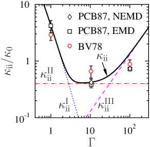
Figure 2: (color online) Dimensionless ion-ion thermal conductivity $\kappa_{\mathrm{ii}}/\kappa_{0}$ for a classical ion plasma ($T\gg T_{\mathrm{p}}$) as a function of $\Gamma$. Circles show results of equilibrium molecular dynamics (EMD) simulations of Bernu & Vieillefosse 1978 (BV 78), squares and diamonds present equilibrium and nonequilibrium molecular dynamics results of (Pierleoni et al.1987) (PCB87 EMD and NEMD), respectively. The solid line is our interpolation, Eq. (26). Dotted, dot-dashed and dashed lines are the conductivities in domains I–III, given by Eqs. (18), (20) and (22), respectively.

To facilitate the implication of the above results we can suggest the following interpolation formula for $\kappa_{\mathrm{ii}}$ in all domains I–V in Fig. 1,

$$\kappa_{\mathrm{ii}} = \left\{\left(\kappa_{\mathrm{ii}}^{\mathrm{I}}\right)^{2}+\left(\kappa_{\mathrm{ii}}^{\mathrm{II}}\right)^{2}+\left(\kappa_{\mathrm{ii}}^{\mathrm{III}\textrm{-}\mathrm{V}}\right)^{2}\right\}^{1/2}$$ (26)

$$= \kappa_{0}\,\left\{\Gamma^{-5}/\ln^{2}\left[2+1/(\sqrt{3}\Gamma^{3/2})\right]\right.$$

$$+ \left.\kappa_{\ast}^{2}+\left(\Gamma/77\right)^{2}\,\exp\left(2\beta T_{\mathrm{p}}/T\right)\right\}^{1/2},$$

with $\kappa_{\ast}\approx 0.4$ and $\beta\approx 1/3$. Here, we assume a smooth temperature variation of $\kappa_{\mathrm{ii}}$, without any jump or break at the melting point $T=T_{\mathrm{m}}$. Our assumption is made in analogy with the electron thermal conductivity which does not show any peculiarity at $T=T_{\mathrm{m}}$ (Baiko et al., 1998) because of the importance of multi-phonon electron-phonon scattering processes in crystalline lattice at $T<T_{\mathrm{m}}$ and because of incipient ion-ion correlations in ion liquid at $T>T_{\mathrm{m}}$. Another argument in favor of a relatively smooth behavior of the conductivity near the melting point is given by the presence of shear modes in a strongly coupled Coulomb liquid (Schmidt et al., 1997), that is typical for a crystal rather than for a liquid.

Figure 2 shows the dependence of a dimensionless thermal conductivity $\kappa_{\mathrm{ii}}/\kappa_{0}$ in a classical ion plasma on the Coulomb coupling parameter $\Gamma$. Circles are the results of Bernu & Vieillefosse (1978) (BV78). Squares and diamonds are calculations of (Pierleoni et al.1987) carried out using equilibrium molecular dynamics and nonequilibrium molecular dynamics techniques (PCB87 EMD and PCB87 NEMD), respectively. Dotted, dot-dashed and dashed lines present the thermal conductivities calculated, respectively, from Eqs. (18), (20) and (22), which are valid in domains I, II and III. Our interpolation (26), plotted by the solid line, is in good agreement with the results of Bernu & Vieillefosse (1978) and (Pierleoni et al.1987). In particular, the interpolation predicts a minimum of $\kappa_{\mathrm{ii}}/\kappa_{0}$ at $\Gamma\sim 7$, which agrees with the estimate of Bernu & Vieillefosse (1978) that the minimum takes place in the vicinity of $\Gamma=10$. The largest, but still acceptable deviation of the interpolated $\kappa_{\mathrm{ii}}/\kappa_{0}$ from the results of Bernu & Vieillefosse (1978) and (Pierleoni et al.1987) occurs at $\Gamma\sim 100$. It can be explained by a significant contribution of multi-phonon processes [neglected in Eq. (22)], as well as by an inaccuracy of Eq. (22), which is just an order-of-magnitude estimate of the thermal conductivity of ions in the crystalline phase that we use to determine the thermal conductivity at $\Gamma=100$ in our interpolation.

5 Phonon conduction due to phonon-electron scattering

Now let us discuss $\kappa_{\mathrm{ie}}$, which is the partial ion thermal conductivity due to ion-electron scattering in Eq. (17). This process was not considered by (Pérez-Azorín et al.2006). As already mentioned above, this mechanism appears to be important only for the crystalline lattice at $T\la T_{\mathrm{m}}$, and becomes negligible at higher $T$ as compared to ion-ion scattering.

5.1 General formalism

We will mainly focus on the case in which $T\lesssim T_{\mathrm{m}}$ and the phonon formalism is appropriate, so that $\kappa_{\mathrm{ie}}$ can be treated as the phonon thermal conductivity produced due to phonon-electron scattering (due to absorptions and emissions of phonons by electrons, ph+e$\to$e and e$\to$ph+e). We expect that the formalism described below is valid for calculating $\kappa_{\mathrm{ie}}$ in temperature-density domains III–V displayed in Fig. 1 and listed in Table 1. The conductivity $\kappa_{\mathrm{ie}}$ can be calculated using the variational method, described, for instance, in Chapter 7 of Ziman (1960). The variational expression reads

$$\kappa_{\mathrm{ie}}={1\over\dot{S}_{\mathrm{coll}}}\;\left|\sum_{s}\int\bm{v}_{\nu}\Phi_{\nu}\frac{\partial n_{\nu}}{\partial T}\,{\rm d}\bm{Q}\right|^{2}.$$ (27)

In this case, $\nu\equiv({\bm{Q}},\,s)$ enumerates phonon modes, $\bm{Q}$ is a phonon wavevector, and $s$ is a polarization index; a phonon frequency will be denoted by $\omega_{\nu}$. Furthermore, $n_{\nu}=1/[\exp(\hbar\omega_{\nu}/k_{\mathrm{B}}T)-1]$ is the phonon equilibrium occupation number, and ${\bm{v}}_{\nu}=\partial\omega_{\nu}/\partial{\bm{Q}}$ is the phonon group velocity; $\dot{S}_{\mathrm{coll}}$ is the entropy generation rate in phonon-electron scattering. A variational function $\Phi_{\nu}$ describes a weak deviation of the phonon distribution function from the equilibrium distribution $n_{\nu}$. The variational estimate of $\kappa_{\mathrm{ie}}$ given by Eq. (27) reaches maximum for the exact solution of the phonon transport equation. For phonon-electron scattering, the entropy generation rate can be expressed as (Ziman 1960, Chapter 8, §9)

$$\dot{S}_{\mathrm{coll}} = \frac{1}{k_{\mathrm{B}}\,T^{2}}\int\Phi_{\bm{Q}}^{2}\mathcal{P}_{{\bm{Q}},{\bm{k}}}^{\bm{k^{\prime}}}{\rm d}{\bm{Q}}\,{\rm d}{\bm{k}}\,{\rm d}\bm{k^{\prime}}.$$ (28)

For the sake of simplicity, polarization indices are omitted here. Wavevectors $\bm{k}$ and ${\bm{k}}^{\prime}$ refer to electrons. In calculating $\kappa_{\mathrm{ie}}$ the electron distributions are assumed to be equilibrium ones. Finally, $\mathcal{P}_{{\bm{Q}},{\bm{k}}}^{{\bm{k}}^{\prime}}$ is the differential transition probability, calculated in equilibrium.

The derivation of $\kappa_{\mathrm{ie}}$ is simplified (Ziman 1960, Chapter 8, §9) by the equality of the squared matrix elements for the phonon absorption and emission processes. Employing the simplest suitable variational function $\Phi_{\nu}=\bm{Q}\cdot\bm{u}$ ($\bm{u}$ being the unit vector along the temperature gradient), one gets

$$\kappa_{\mathrm{ie}}=\left(\frac{k_{\mathrm{B}}\,C_{\mathrm{i}}}{3\,Z\,e}\right)^{2}\,T\,\widetilde{\sigma},$$ (29)

where

$$\widetilde{\sigma}=\frac{e^{2}\,n_{\mathrm{e}}\widetilde{\tau}_{\sigma}}{m^{\ast}_{e}},\quad\widetilde{\tau}_{\sigma}=\frac{p_{\mathrm{F}}^{2}v_{\mathrm{F}}}{4\pi\,Z^{2}e^{2}\,n_{\mathrm{i}}\widetilde{\Lambda}_{\mathrm{e}}},$$ (30)

are auxiliary quantities, which are formally similar (but not identical) to the electron electric conductivity and the electron effective relaxation time due to electron-photon scattering, and

$$\widetilde{\Lambda}_{\mathrm{e}} = \frac{2\,p_{\mathrm{F}}^{2}}{m_{\mathrm{i}}k_{\mathrm{B}}T}\,\int\frac{{\rm d}\Omega_{\bm{k}}}{4\pi}\,\int\frac{{\rm d}\Omega_{\bm{k^{\prime}}}}{4\pi}\left|\phi(q)\right|^{2}\,$$ (31)

$$\times \left[1-\frac{v_{\mathrm{F}}^{2}}{c^{2}}\,\left(\frac{q}{2k_{\mathrm{F}}}\right)^{2}\right]\,Q^{2}\,\exp[-W(q)]$$

$$\times \sum_{s}({\bm{q}}\cdot\bm{e}_{\nu})^{2}\,\frac{\exp(-z_{\nu})}{\left[1-\exp(-z_{\nu})\right]^{2}}.$$

is formally similar to the Coulomb logarithm for the electron transport [although it differs from the real Coulomb logarithm that contains $q^{2}$ instead of $Q^{2}$; see, e.g., Baiko & Yakovlev 1995]. Since $\widetilde{\sigma}$ and $\widetilde{\tau}_{\sigma}$ are not real electric conductivity and relaxation time, $\kappa_{\mathrm{ie}}$ and $\widetilde{\sigma}$ do not obey the Wiedemann-Franz law. The integration in (31) is done over positions of both electrons on the Fermi surface, with wavevectors $\bm{k}$ and $\bm{k^{\prime}}$ ($\mathrm{d}\Omega_{\bm{k}}$ and $\mathrm{d}\Omega_{\bm{k^{\prime}}}$ are respective solid angle elements). Furthermore, $\bm{q}=\bm{k}-\bm{k^{\prime}}$ is an electron momentum transfer in a scattering event, and $\bm{Q}$ is the phonon wavevector that is equal to $\bm{q}$ reduced to the first Brillouin zone (see Chapter 1 of Ziman 1960 for more details). Specifically, $\bm{Q}=\bm{q}-\bm{g}$, where $\bm{g}$ is a reciprocal lattice vector which realizes such a reduction (absorbs a momentum excess). Let us remind that the processes with $\bm{g}\neq\bm{0}$ belong to Umklapp phonon-electron scattering processes, while the processes with $\bm{g}=\bm{0}$ are normal phonon-electron processes. The quantity $\left|\phi(q)\right|\approx F(q)/(q^{2}+k_{\mathrm{TF}}^{2})$ in Eq. (31) is a Fourier transform of the screened Coulomb electron-ion interaction; $k_{\mathrm{TF}}$ is the Thomas-Fermi screening wavenumber given by Eq. (9); $F(q)$ is the nucleus form factor which accounts for the proton charge distribution within the atomic nucleus; $W(q)$ is the doubled Debye-Waller factor (see, e.g., Baiko & Yakovlev 1995). In addition, we have defined $z_{\nu}=\hbar\omega_{s}(\bm{Q})/k_{\mathrm{B}}T$ and the phonon polarization vector $\bm{e}_{\nu}=\bm{e}_{s}({\bm{Q}})$.

We have performed extensive computations of $\widetilde{\Lambda}_{\mathrm{e}}$ and $\kappa_{\mathrm{ie}}$ from Eqs. (29)–(31) by the Monte Carlo technique. In these calculations, the positions of electrons ($\bm{k}$ and $\bm{k^{\prime}}$) on the Fermi surface are randomly selected at every step in long Monte Carlo runs. For every selection, we calculate $\bm{q}$, a respective inverse lattice vector $\bm{g}$, and a phonon wavevector $\bm{Q}$. The phonon eigenfrequencies $\omega_{s}(\bm{Q})$ and polarization vectors $\bm{e}_{s}(\bm{Q})$ have been determined then for a Coulomb crystal of ions immersed in the rigid electron background (see, e.g., Baiko et al. 2001). Small (but finite) widths of energy gaps in electron energy spectrum at the intersections of the electron Fermi surface with boundaries of Brillouin zones have been neglected. We have calculated $\kappa_{\mathrm{ie}}$ for body-centered cubic and face-centered cubic crystals, and the results turn out to be the same. The same conclusions have been reached by Baiko et al. (1998) with regard to the electron transport coefficients determined by electron-phonon scattering.

When the temperature decreases, the number of phonons, which can efficiently participate in phonon-electron scattering, becomes smaller. They can only be the phonons with small frequencies [$\hbar\omega_{s}(\bm{Q})\sim k_{\mathrm{B}}T$] and, hence, with small wavevectors $\bm{Q}$ near the center of the Brillouin zone. The regions on the Fermi surface, which mainly contribute to the integral (31), become narrower, and the accuracy of our direct Monte Carlo calculations gets lower. At sufficiently low $T$ direct Monte Carlo calculation is inefficient and we replace it with a semi-analytic consideration (Sect. 5.2). In Fig. 1, the $T-\rho$ domains, where direct Monte Carlo calculations are effective, are labeled as III and IV, while domain V will be described semi-analytically. We combine Monte Carlo and semi-analytic results and produce a useful practical fit expression in Sect. 5.3.

5.2 Umklapp processes at low temperatures

Let us analyze phonon-electron Umklapp processes (${\bm{g}}\neq\bm{0}$) at low temperatures (domain V in Fig. 1). In this case it is sufficient to consider small phonon wavenumbers $Q\ll q_{\mathrm{BZ}}$, and we can rewrite Eq. (31) in the form

$$\widetilde{\Lambda}^{\rm U}_{\mathrm{e}} = \frac{p_{\mathrm{F}}^{2}}{8\,\pi^{2}\,m_{\mathrm{i}}k_{\mathrm{B}}T}\sum_{g<2k_{\mathrm{F}}}\frac{F^{2}(g)}{g^{4}}\,\left[1-\frac{v_{\mathrm{F}}^{2}}{c^{2}}\,\left(\frac{g}{2k_{\mathrm{F}}}\right)^{2}\right]$$ (32)

$$\times \exp[-W(q)]I_{\bm{g}},$$ (34)

$$I_{\bm{g}} = \int{\rm d}\Omega_{\bm{k}}\,{\rm d}\Omega_{\bm{k^{\prime}}}\,Q^{2}\,\sum_{s}({\bm{g}}\cdot{\bm{e}}_{\nu})^{2}\,\frac{\exp(-z_{\nu})}{\left[1-\exp(-z_{\nu})\right]^{2}},$$ (35)

where the sum is over all non-zero reciprocal lattice vectors inside the Fermi sphere ($g<2k_{\mathrm{F}}$). Using symmetry properties, one can show that $(\bm{g}\cdot\bm{e}_{\nu})^{2}$ in the integrand can be replaced by $g^{2}/3$.

At low temperatures we are interested in, the main contribution into $I_{\bm{g}}$ comes from those positions of $\bm{k}$ and $\bm{k^{\prime}}$ on the Fermi sphere, for which $\bm{k}-\bm{k^{\prime}}\approx\bm{g}$. This case can be studied semianalytically following Pethick & Thorsson (1997) who considered analogous problem in the neutrino emission due to electron-nucleus collisions. Let us introduce a coordinate system whose $z$ axis is directed along $\bm{g}$. Let us further define $\bm{k}$ by its polar and azimuthal angles $\vartheta$ and $\varphi$, and $\bm{k^{\prime}}$ by its polar and azimuthal angles $\vartheta^{\prime}$ and $\varphi^{\prime}$, and introduce $\mu=\cos\vartheta$, $\mu^{\prime}=\cos\vartheta^{\prime}$. The allowed positions of $\bm{k}$ should concentrate on a ring ($0\leq\varphi<2\pi$) with $\mu\approx\mu_{0}=g/(2k_{\mathrm{F}})$; while the respective positions of $\bm{k^{\prime}}$ should concentrate on a complementary ring ($\varphi^{\prime}\approx\varphi\equiv\varphi_{0}$, $\vartheta^{\prime}\approx\pi-\vartheta$). Let $\bm{k}_{0}$ be a position of $\bm{k}$ exactly on the ring, and $\bm{k^{\prime}}_{0}=\bm{k}_{0}-\bm{g}$ be a respective ($\varphi^{\prime}=\varphi$) position of $\bm{k^{\prime}}$ on the complementary ring. Small variations of $\bm{k}$ and $\bm{k^{\prime}}$ around these positions can be defined by $\Delta\mu=\mu-\mu_{0}$, $\Delta\mu^{\prime}=\mu^{\prime}-\mu^{\prime}_{0}$, $\Delta\varphi^{\prime}=\varphi^{\prime}-\varphi_{0}$, $\Delta{\bm{k}}=\bm{k}-\bm{k}_{0}$, and $\Delta\bm{k^{\prime}}=\bm{k^{\prime}}-\bm{k^{\prime}}_{0}$. Using cylindrical coordinates, we get then

$$\Delta k_{||}\approx k_{\mathrm{F}}\,\Delta\mu,\quad\Delta k_{\bot}\approx-\frac{\mu_{0}}{\sqrt{1-\mu_{0}^{2}}}\,k_{\mathrm{F}}\,\Delta\mu, \Delta k_{\varphi}=0,$$ (36)

$$\Delta k_{||}^{\prime}\approx k_{\mathrm{F}}\,\Delta\mu^{\prime},\quad\Delta k_{\bot}^{\prime}\approx\frac{\mu_{0}}{\sqrt{1-\mu_{0}^{2}}}\,k_{\mathrm{F}}\,\Delta\mu^{\prime},$$ (38)

$$\Delta k_{\varphi}^{\prime}\approx\sqrt{1-\mu_{0}^{2}}\,k_{\mathrm{F}}\Delta\varphi^{\prime}.$$ (40)

Because the phonon wavevector is $\bm{Q}=\Delta{\bm{k}}-\Delta{\bm{k}}^{\prime}$, we obtain

$$Q_{||} \approx k_{\mathrm{F}}\,\left(\Delta\mu^{\prime}+\Delta\mu\right),\quad$$ (41)

$$Q_{\bot} \approx \frac{\mu_{0}}{\sqrt{1-\mu_{0}^{2}}}\,k_{\mathrm{F}}\,\left(\Delta\mu^{\prime}-\Delta\mu\right),$$ (43)

$$Q_{\varphi} \approx -\sqrt{1-\mu_{0}^{2}}\,k_{\mathrm{F}}\,\Delta\varphi^{\prime}.$$ (45)

The Jacobian of the transformation from variables $(\Delta\mu,\,\Delta\mu^{\prime},\,\Delta\varphi^{\prime})$ to $(Q_{||},\,Q_{\bot},\,Q_{\varphi})$ is $1/{2\,\mu_{0}k_{\mathrm{F}}^{3}}$. It is then easy to pass from coordinates $(Q_{||},\,Q_{\bot},\,Q_{\varphi})$ to spherical coordinates of the vector $\bm{Q}$. Because only small-$Q$ phonons are available in the cold crystal, we can safely extend the integration over $Q$ to infinity. As a result, we obtain

$$I_{\bm{g}} = \frac{g}{3\,k_{\mathrm{F}}^{2}}\,\int_{0}^{2\pi}{\rm d}\varphi\sum_{s}\int{\rm d}\Omega_{\bm{Q}}\int_{0}^{\infty}{\rm d}Q\,Q^{4}\,$$ (46)

$$\times\,\frac{\exp(-z_{\nu})}{\left[1-\exp(-z_{\nu})\right]^{2}}.$$ (48)

At $Q\ll q_{\mathrm{BZ}}$ in the Coulomb crystal we have two nearly acoustic phonon modes ($z_{1,\,2}\approx\hbar\,c_{1,\,2}(\hat{\bm{Q}})\,Q/k_{\mathrm{B}}T$, $\hat{\bm{Q}}$ being a unit vector along $\bm{Q}$) and one nearly optical mode ($z_{3}\approx\hbar\omega_{\mathrm{p}}/k_{\mathrm{B}}T\gg 1$) that does not contribute to $I_{\bm{g}}$. The integration over ${\rm d}Q$ for acoustic modes gives

$$\int_{0}^{\infty}Q^{4}\,\frac{\exp(-z_{1,\,2})}{\left[1-\exp(-z_{1,\,2})\right]^{2}}\,{\rm d}Q = 4!\,\zeta(4)\,\left[\frac{k_{\mathrm{B}}\,T}{\hbar\,c_{1,\,2}(\hat{\bm{Q}})}\right]^{5}=$$ (49)

$$\quad=\frac{4\pi^{4}}{15}\,\left[\frac{k_{\mathrm{B}}\,T}{\hbar\,c_{1,\,2}(\hat{\bm{Q}})}\right]^{5},$$ (51)

and the integral over $\varphi$ gives $2\pi$. Therefore,

$$I_{\bm{g}} = \frac{8\pi^{5}}{45}\,\left(\frac{k_{\mathrm{B}}\,T}{\hbar}\right)^{5}\frac{g}{k_{\mathrm{F}}^{2}}\sum_{s=1,\,2}\int{\rm d}\Omega_{\bm{Q}}\,c_{s}^{-5}\,=$$ (52)

$$= \frac{64\pi^{6}}{45}\,\left(\frac{k_{\mathrm{B}}\,T}{\hbar\,\overline{{c_{\mathrm{s}}}}}\right)^{5}\,\frac{g}{k_{\mathrm{F}}^{2}},$$ (54)

where

$$\overline{c}_{\mathrm{s}}\equiv\left({1\over 8\pi}\,\sum_{s}\int{\rm d}\Omega_{\bm{Q}}\,c_{s}^{-5}\right)^{-1/5}$$ (55)

is an average phonon group speed that can be written as $\overline{{c_{\mathrm{s}}}}={\cal A}\,\omega_{\mathrm{p}}/q_{\mathrm{BZ}}$. The calculation yields ${\cal A}\approx 0.36$ for both bcc and fcc Coulomb crystals. Finally, we have

$$\widetilde{\Lambda}^{\mathrm{U}}_{\mathrm{e}} = \frac{\pi^{4}}{45}\,\frac{\hbar\,q_{\mathrm{BZ}}^{2}}{m_{\mathrm{i}}\,\omega_{\mathrm{p}}}\,\left(\frac{q_{\mathrm{BZ}}}{k_{\mathrm{F}}}\right)^{3}\,{1\over{\cal A}^{5}}\,\left(T\over T_{\mathrm{p}}\right)^{4}\sum_{g<2k_{\mathrm{F}}}F^{2}(g)\times$$ (56)

$$\times \left(\frac{2k_{\mathrm{F}}}{g}\right)^{3}\left[1-\frac{v_{\mathrm{F}}^{2}}{c^{2}}\,\left(\frac{g}{2k_{\mathrm{F}}}\right)^{2}\right]\,\exp[-W(q)].$$ (58)

As in the case of electron transport (see, e.g., Potekhin et al. 1999), normal phonon-electron processes give small contribution into scattering rate and can be neglected. The same is true for higher temperatures.

Notice in passing, that in the same manner we can obtain an asymptotic form of the Coulomb logarithm for the electron electrical conductivity due to electron-phonon scattering,

$${\Lambda^{\sigma}_{\mathrm{U}}} = \frac{\pi^{2}}{9}\,\frac{\hbar\,q_{\mathrm{BZ}}^{2}}{m_{\mathrm{i}}\,\omega_{\mathrm{p}}}\,\frac{q_{\mathrm{BZ}}}{k_{\mathrm{F}}}\,{1\over{\cal A^{\prime}}^{3}}\,\left(T\over T_{\mathrm{p}}\right)^{2}\sum_{g<2k_{\mathrm{F}}}F^{2}(g)\,\frac{2k_{\mathrm{F}}}{g}$$ (59)

$$\times \,\left[1-\frac{v_{\mathrm{F}}^{2}}{c^{2}}\,\left(\frac{g}{2k_{\mathrm{F}}}\right)^{2}\right]\,\exp[-W(q)].$$ (61)

However, in this case an effective phonon group velocity is $\overline{{c_{\mathrm{s}}}^{\prime}}={\cal A}^{\prime}\,\omega_{\mathrm{p}}/q_{\mathrm{BZ}}$ with ${\cal A}^{\prime}\approx 0.40$ for both bcc and fcc lattices. The difference in the values of ${\cal A}$ and ${\cal A}^{\prime}$ results from averaging different powers of ${c_{\mathrm{s}}}(\hat{\bm{Q}})$. Our asymptotic expression for ${\Lambda^{\sigma}_{\mathrm{U}}}$ agrees with previous calculations (e.g., Gnedin et al.2001).

5.3 Interpolation expression

In order to approximate the thermal conductivity $\kappa_{\mathrm{ie}}$ in domains III–V we present it in the familiar form

$$\kappa_{\mathrm{ie}}=\frac{1}{3}\,k_{\mathrm{B}}\,C_{\mathrm{i}}n_{\mathrm{i}}{c_{\mathrm{s}}}L_{\mathrm{ph}}^{\mathrm{ie}},$$ (62)

with ${c_{\mathrm{s}}}=\omega_{\mathrm{p}}/(3q_{\mathrm{BZ}})$. We have extracted the mean free path $L_{\mathrm{ph}}^{\mathrm{ie}}$ from our numerical calculations and obtained that it can be described by a slowly variable function of $\theta=T_{\mathrm{p}}/T$ which we denote by $F(\theta)$. Its density dependence has been approximated by replacing the sum over reciprocal lattice vectors $\bm{g}$ in the asymptotic expression (56) with the integral over the vectors $\bm{g}$ uniformly distributed within the spherical layer of the inner radius $q_{\mathrm{BZ}}$ and the outer radius $2\,k_{\mathrm{F}}$. Then, the Coulomb logarithm $\widetilde{\Lambda}^{\mathrm{U}}_{\mathrm{e}}$ has been adjusted to the mean free path $L_{\mathrm{ph}}^{\mathrm{ie}}$ using Eqs. (29), (30), and (62). While integrating, we have used the Debye-Waller factor which corresponds to a given temperature. In analogy with the approximation of the electron thermal conductivity by (Gnedin et al.2001), the effect of the nucleus form factor has been taken into account by introducing into the integrand an additional factor $\exp\left(w_{\mathrm{form}}\,g^{2}/4\,k_{\mathrm{F}}^{2}\right)$. As a result, the mean free path has been approximated as

$$L_{\mathrm{ph}}^{\mathrm{ie}} = \frac{3}{2}\,\frac{m_{\mathrm{i}}\,\omega_{\mathrm{p}}\,p_{\mathrm{F}}^{2}\,v_{\mathrm{F}}}{Z^{2}e^{4}\,m_{\mathrm{e}}^{\ast}\,q_{\mathrm{BZ}}\,n_{\mathrm{e}}}\,\frac{F(\theta)}{\Lambda_{\mathrm{ph\,e}}}$$ (63)

$$\approx \frac{320\,a_{\mathrm{i}}}{\left(1+x_{\mathrm{r}}^{2}\right)\Lambda_{\mathrm{ph\,e}}}\,\frac{26}{Z}\,\frac{F(\theta)}{0.01}\left(\frac{A\,\rho_{6}}{A^{\prime}}\right)^{1/2},$$ (65)

where

$$2\,\Lambda_{\mathrm{ph\,e}} = E_{1}(w\,y^{2})-E_{1}(w)-\frac{v_{\mathrm{F}}^{2}}{c^{2}}\frac{\mathrm{e}^{-w\,y^{2}}-\mathrm{e}^{-w}}{w}\leavevmode\nobreak\ ,$$ (66)

$$F(\theta) = 0.014+\frac{0.03}{\exp(\theta/5)+1},$$ (67)

$w=w_{\mathrm{DW}}+w_{\mathrm{form}}$, and $y=q_{\mathrm{BZ}}/(2k_{\mathrm{F}})=(4Z)^{-1/3}$. The quantity

$$w_{\mathrm{DW}}=1.683\,\sqrt{\frac{x_{\mathrm{r}}}{AZ}}\,\left[0.5\,u_{-1}\,\exp(-9.1/\theta)+u_{-2}/\theta\right]$$ (68)

measures the efficiency of the Debye-Waller factor (Baiko & Yakovlev 1995); $w_{\mathrm{form}}$ determines the importance of the form factor of atomic nuclei (see, e.g., Gnedin et al.2001); $u_{-1}\approx 2.8$ and $u_{-2}\approx 13.0$ are dimensionless phonon frequency moments (e.g., Pollock & Hansen 1973); $E_{1}(x)=\int_{x}^{\infty}y^{-1}\exp(-y)\,{\rm d}y$ is the standard exponential integral (whose approximations are given by Abramowitz & Stegun 1972).

Now let us employ the ground-state composition of crustal matter and the corresponding smooth composition model to describe proton charge distribution within atomic nuclei in the crust (see Sect. 2 and Appendix B of Haensel et al.2007). The radial dependence of the proton number density within the proton core of the nucleus ($r<R_{\mathrm{p}}$) is $n_{\mathrm{p}}(r)\propto\left[1-(r/R_{\mathrm{p}})^{t_{\mathrm{p}}}\right]^{3}$, where $R_{\mathrm{p}}$ and $t_{\mathrm{p}}$ are density dependent parameters. In order to describe the effect of the nuclear form factor it is sufficient to set

$$w_{\mathrm{form}}=43\,x_{\mathrm{nuc}}^{2},$$ (69)

where

$$x^{2}_{\mathrm{nuc}}=\frac{R_{\mathrm{p}}^{2}}{a_{\mathrm{i}}^{2}}\frac{1-15/(5+t_{\mathrm{p}})+15/(5+2t_{\mathrm{p}})-5/(5+3t_{\mathrm{p}})}{1-9/(3+t_{\mathrm{p}})+9/(3+2t_{\mathrm{p}})-1/(1+t_{\mathrm{p}})}$$ (70)

(Haensel et al.2007, Appendix B). Notice that the nucleus form factor and the associated parameter $w_{\mathrm{form}}$ are important only in inner crust, where the phonon conductivity is rather insignificant. In the outer crust, one can set $w_{\mathrm{form}}=0$.

We have calculated $\kappa_{\mathrm{ie}}$ on a dense grid of $T$ and $\rho$ values ($\log_{10}T\leavevmode\nobreak\ [\mathrm{K}]$ from 5 to 9, with the step of 0.2; $\log_{10}\rho\leavevmode\nobreak\ [\mathrm{g\leavevmode\nobreak\ cm}^{-3}]$ from 5 to 14, with the step of 0.1) restricted by the condition $\Gamma\geq 30$. The root mean square relative fit error is 8%, and the maximum error $\approx 25$% takes place at $T=6\times 10^{7}$ K and $\rho=4\times 10^{12}$ g cm^-3. Had we restricted ourselves to the outer crust ($\rho\leq 4.3\times 10^{11}$ g cm^-3), where the phonon thermal conductivity can be really significant, then the root mean square relative error would be 7%, and the maximum error of 21% would occur at $T=4\times 10^{7}$ K and $\rho=2.5\times 10^{11}$ g cm^-3. For $\Gamma<\Gamma_{\mathrm{m}}\approx 175$ (the shaded region in Fig. 3) ions form a strongly non-ideal Coulomb liquid, and the crystal-phonon description is, strictly speaking, invalid. Nevertheless, as far as transport properties are concerned, a strongly coupled Coulomb liquid has much in common with a Coulomb crystal (see, e.g., Schmidt et al. 1997, Baiko et al. 1998, Haensel et al.2007). Therefore, we have extended calculations (and included them in the fit) to $\Gamma=30$, because we expect that for $30\lesssim\Gamma<175$ the adopted formalism still gives correct order-of-magnitude estimates of the phonon-electron thermal conductivity in the ion liquid (which is the thermal conductivity of strongly coupled ions). Let us remind, that the electron transport coefficients behave smoothly near the melting point (e.g., Potekhin et al. 1999).

In fact, near the melting point (at $\Gamma\lesssim 175$) phonon-electron scattering becomes unimportant for ion conduction (see Fig. 1 and Table 1) and an uncertainty of our approximation of $\kappa_{\mathrm{ie}}$ does not affect the accuracy of the evaluation of the total ion conductivity $\kappa_{\mathrm{i}}$. A formal extension of our fit expression (63) to low $\Gamma\lesssim 30$ leads to an unrealistic exponential freezing of the ion-electron scattering (an exponential growth of $\kappa_{\mathrm{ie}}$), which does not affect $\kappa_{\mathrm{i}}$ determined by ion-ion scattering.

Let us remark that if we neglect the Debye-Waller factor ($w_{\mathrm{DW}}=0$) and the nuclear form factor ($w_{\mathrm{form}}=0$), then we obtain

$$\Lambda_{\mathrm{ph\,e}}\approx\,\ln\left(2\,k_{\mathrm{F}}\over q_{\mathrm{BZ}}\right)-\frac{v_{\mathrm{F}}^{2}}{2c^{2}}\,\left(1-\frac{q_{\mathrm{BZ}}^{2}}{4\,k_{\mathrm{F}}^{2}}\right).$$ (71)

Accordingly, $\Lambda_{\mathrm{ph\,e}}$ can be treated as a familiar Coulomb logarithm (which takes into account a suppression of backscattering for relativistic electrons) with the minimum electron momentum transfer of $q_{\mathrm{BZ}}$ and the maximum momentum transfer of $2\,k_{\mathrm{F}}$.

6 Anisotropy of ion heat conduction

Let us estimate magnetic field strengths which make ion heat transport anisotropic. In a weakly coupled Coulomb plasma ($\Gamma\ll 1$) the effect of the magnetic field on the ion thermal conductivity is well known (e.g., Braginski 1963). Specifically, the magnetic field does not affect noticeably the ion transport as long as the ion magnetization parameter is small, $\omega_{B\mathrm{i}}\tau_{\mathrm{i}}\lesssim 1$, where $\omega_{B\rm i}=ZeB/(m_{\mathrm{i}}c)$ is the ion cyclotron frequency.

In a Coulomb crystal or liquid, we expect that the magnetic field strongly influences ion heat transport provided it distorts the spectrum of heat carrying phonons. In a classical crystal ($T\gtrsim T_{\mathrm{p}}/3$) the heat is carried by all phonons whose spectrum is distorted when $\omega_{B\mathrm{i}}\gtrsim\omega_{\mathrm{p}}$ (Baiko 2000; Haensel et al.2007, § 4.1.6b). The latter inequality will be treated as a condition for an anisotropic ion thermal conductivity; we will use it for ion liquid and solid. In the quantum crystal ($T\ll T_{\mathrm{p}}$) heat is mainly transported by low-frequency phonons (Sec. 5.2), with $\omega\sim\omega_{T}\sim k_{\mathrm{B}}T/\hbar$. Their spectrum is affected by the magnetic field at $\omega_{B\mathrm{i}}\gtrsim\omega_{T}$ (Baiko 2000; Haensel et al.2007, §4.1.6b). Accordingly, the criterion for anisotropic ion conduction can be written as $\omega_{B\mathrm{i}}\gtrsim\omega_{\mathrm{p}}\,T/T_{\mathrm{p}}$. The same criteria can be applied for describing the effects of the magnetic field on the thermodynamic properties of Coulomb crystal. They are in a qualitative agreement with the results of accurate calculations (Baiko 2000; Haensel et al.2007, §4.1.6b, their Fig. 4.3), which can serve as an additional argument in favor of our criterion.

Basing on the above estimates we can introduce a characteristic magnetic field $B_{\mathrm{m}}$, which starts to affect ion heat transport and makes this transport anisotropic. At $B\lesssim B_{\mathrm{m}}$ one can neglect the effect of the magnetic field on $\kappa_{\mathrm{i}}$ and use the results of preceding sections. We can suggest a simple estimate of $B_{\mathrm{m}}$; it is valid in a wide range of densities and temperatures including all values of $\rho$ and $T$ shown in Fig. 1,

$$B_{\mathrm{m}} = \frac{m_{\mathrm{i}}c}{Ze}\,\left(\tau_{\mathrm{ii}}^{2}+\frac{1}{\omega_{\mathrm{p}}^{2}}+\frac{1}{\omega_{T}^{2}}\right)^{-1/2}\approx 10^{14}\,\left(\rho_{6}\,A/A^{\prime}\right)^{1/2}\,$$ (72)

$$\times \left[3\pi\,\Gamma^{-3}/\Lambda_{\mathrm{ii}}^{2}+1+\left(T_{\mathrm{p}}/T\right)^{2}\right]^{-1/2}\,\mathrm{G},$$

where $\tau_{\mathrm{ii}}$ is given by Eq. (19) with the Coulomb logarithm $\Lambda_{\mathrm{ii}}=\ln\left[2+1/(\sqrt{3}\Gamma^{3/2})\right]$. The magnetic field $B\gtrsim 10^{14}\,\rho_{6}^{1/2}$ G, for which $\omega_{B\mathrm{i}}\gtrsim\omega_{\mathrm{p}}$, strongly affects ion heat transport at any temperature. At lower field $B$, the condition $B\sim B_{\mathrm{m}}$ is realized at sufficiently low or sufficiently high temperatures. In the case of low temperatures, a magnetized Coulomb crystal possesses very soft phonon modes which are responsible for heat transport and most sensitive to the magnetic field (Baiko 2000; Haensel et al.2007, §4.1.6b, Fig. 4.3). In the high temperature plasma, the ions become weakly coupled and their relaxation time (19) rapidly increases with the growth of $T$, increasing a typical rotation angle of ions between successive collisions, and hence the magnetic field effect.

The boundaries of domains, where $B\gtrsim B_{\mathrm{m}}$ and $\kappa_{\mathrm{i}}$ is anisotropic, are shown in Fig. 1 for $B_{\mathrm{m}}=10^{13}$ and $B_{\mathrm{m}}=10^{14}$ G. The domains themselves are situated below and to the left of these boundaries. A not very strong field $B=3\times 10^{12}$ G (employed in Figs. 3 and 5) does not affect ion conduction at all $T$ and $\rho$ in Fig. 1.

Let us notice that at rather low densities $\rho\lesssim\rho_{B\mathrm{e}}$ (see Sec. 3.1) the plasma electrons occupy only one or several Landau levels. This circumstance can strongly modify electron-phonon scattering. We have neglected this effect in the present publication. However, at these low densities the ion thermal conductivity (at not too low temperatures $T\gtrsim 10^{6}K$) is mainly determined by ion-ion scattering (see Fig. 1) and electron-phonon scattering is relatively unimportant. At high densities the electrons populate many Landau levels so that the Landau level structure can be neglected as confirmed by calculations of electron transport properties (Potekhin, 1999).

7 Discussion

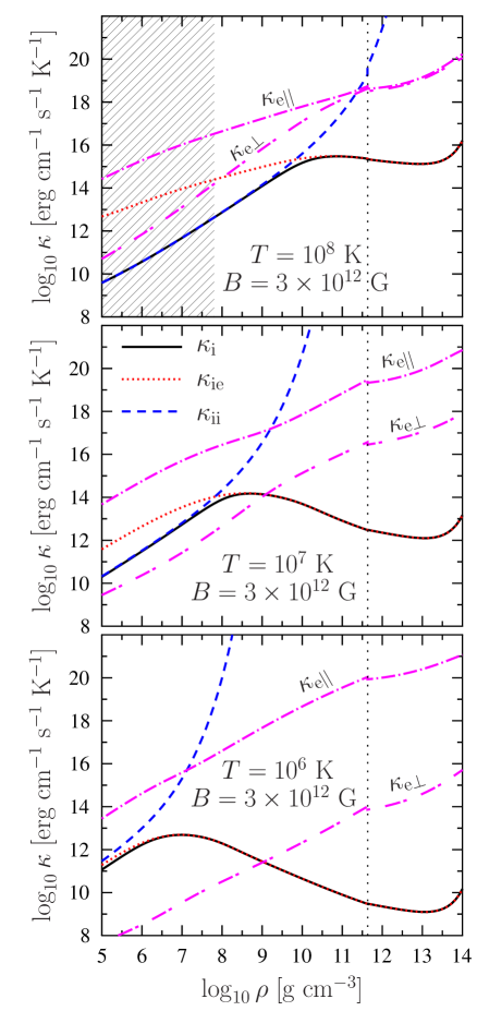
Figure 3: (Color online) Thermal conductivity of the ground-state neutron star crust for $T=10^{6}$, $10^{7}$, and $10^{8}$ K. The solid line is the total ion (phonon) conductivity $\kappa_{\mathrm{i}}$. The dash and dot lines show $\kappa_{\mathrm{ie}}$ and $\kappa_{\mathrm{ii}}$, respectively. The dot-dash lines are the electron thermal conductivities, across and along the magnetic field $B=3\times 10^{12}$ G, calculated using a simplified model of Sect. 3.1. The vertical dotted line shows the neutron drip density $\rho_{\mathrm{ND}}=4.3\times 10^{11}$ g cm^-3. The shaded zone in the upper panel corresponds to a strongly coupled Coulomb liquid ($T>T_{\mathrm{m}}$, see Fig. 1). At $T=10^{7}$ and $10^{6}$ K the ions form a crystal for all displayed densities.

Let us compare the ion thermal conductivity (calculated neglecting the effects of the magnetic field, as discussed in Sect. 3) with the electron thermal conductivities (16) along and across the magnetic field $\bm{B}$.

Figure 3 shows the density dependence of the partial ion conductivities $\kappa_{\mathrm{ii}}$ and $\kappa_{\mathrm{ie}}$, the total ion conductivity $\kappa_{\mathrm{i}}$, and also of the electron conductivities along and across $\bm{B}=3\times 10^{12}\leavevmode\nobreak\ {\rm G}$, $\kappa_{\mathrm{e\parallel}}$ and $\kappa_{\mathrm{e\perp}}$, at three values of $T=10^{6}$, $10^{7}$ and $10^{8}$ K. One sees that the longitudinal electron thermal conductivity $\kappa_{\mathrm{e\parallel}}$ always dominates over the thermal conductivity of ions. Therefore, the ion conductivity cannot contribute into heat transport along magnetic field lines under typical conditions in neutron star envelopes. Nevertheless, it can compete with $\kappa_{\mathrm{e\perp}}$ and be the dominant thermal conductivity across the magnetic field lines, especially at not too high densities (in the outer neutron star envelope) and temperatures. For instance, at $B=3\times 10^{12}$ G and $T=10^{8}$ K (the upper panel in Fig. 3) $\kappa_{\mathrm{i}}$ does not dominate in the transverse conduction at all, but at $T=10^{6-7}$ K (the middle and bottom panels) it dominates in the outer layer at densities $\rho\lesssim 10^{9}$ g cm^-3. This density range is most important in the neutron star physics because it belongs to the neutron-star heat blanketing envelope which shields warm neutron star interior from the efficient cooling via thermal conduction to the surface and then through the thermal emission from the surface (see, e.g., Haensel et al.2007). Higher magnetic fields would stronger suppress $\kappa_{\mathrm{e\perp}}$ and widen the density range where ion thermal conduction across $\bm{B}$ dominates over electron one.

It is important to emphasize the efficiency of phonon-electron scattering (neglected by Pérez-Azorín et al.2006). This scattering is most efficient and determines $\kappa_{\mathrm{i}}$ at sufficiently high densities and low temperatures (in domains IV and V in Fig. 1), while phonon-phonon (ion-ion) scattering overtakes ion transport at lower densities and higher temperatures (in domains I–III). Phonon-electron scattering reduces the total ion conductivity $\kappa_{\mathrm{i}}$ in comparison with the conductivity $\kappa_{\mathrm{ii}}$ that is solely determined by phonon-phonon scattering. In particular, for $B=3\times 10^{12}$ G and $T=10^{8}$ K (the upper panel in Fig. 3) this suppression is very efficient at $\rho\gtrsim 3\times 10^{10}$ g cm^-3. When the star cools, phonon-electron scattering becomes more important, and the layer of its dominance expands to lower $\rho$. For instance, at $T=10^{6}$ K (the bottom panel of Fig. 3) it dominates at all densities (see also Fig. 1).

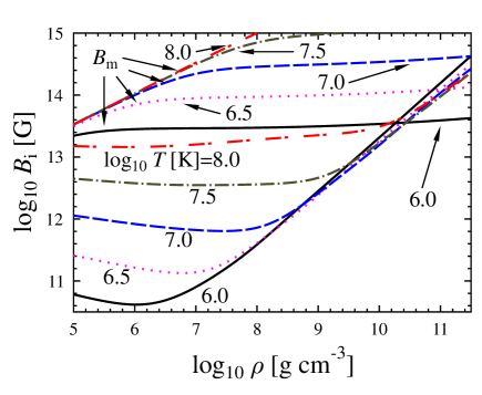
Figure 4: (color online) Characteristic magnetic field $B_{\mathrm{i}}$, which makes the ion thermal conductivity $\kappa_{\mathrm{i}}$ larger than the transverse electron thermal conductivity $\kappa_{e\perp}$, and characteristic field $B_{\mathrm{m}}$, which makes ion thermal conduction anisotropic, versus density, for five values of the temperature with $\log_{10}T[K]=6.0$, 6.5, 7.0, 7.5 and 8.0.

If we fix $\rho$ and $T$ and increase $B$ then the heat transport across $\bm{B}$ will be determined by ions ($\kappa_{\mathrm{i}}\gtrsim\kappa_{\mathrm{e\perp}}$) after $B$ exceeds some value $B_{\mathrm{i}}$. Figure 4 shows the density dependence of $B_{\mathrm{i}}$. At low $\rho$, this density dependence is weak but $B_{\mathrm{i}}$ is a strong function of the temperature (noticeably decreases with decreasing $T$). At large $\rho$, the field $B_{\mathrm{i}}$ becomes almost independent of $T$ (all curves in Fig. 4 merge into nearly one curve) but increases with growing $\rho$. For instance, one needs an ordinary pulsar magnetic field $B\gtrsim 10^{12}$ G for the ion conduction to dominate over $\kappa_{\mathrm{e\perp}}$ at $\rho=10^{9}$ g cm^-3 (for $T\lesssim 10^{7}$ K). However, the neutron star must have a typical magnetar field $B\gtrsim 10^{14}$ G to reach similar dominance at $\rho\sim 10^{11}$ g cm^-3 (for all temperatures in Fig. 4). Also, in Fig. 4 we show the values of the magnetic fields, $B_{\mathrm{m}}$, which make ion heat transport anisotropic for the same temperatures $T$. At not too high densities, $\rho\lesssim 10^{10}$ g cm^-3, the ions become the leading heat carriers across the magnetic fields $B\lesssim B_{\mathrm{m}}$. However, at $\rho\sim 10^{11}$ g cm^-3 the magnetic field $B\gtrsim 10^{14}$ G, which makes the transverse ion heat transport dominant, becomes larger than $B_{\mathrm{m}}$ if the temperatures falls below $T\sim 10^{6}$ K. However, even in that case it would be preferable to use the ion thermal conductivity at $B=0$ than to neglect the ion thermal conductivity at all.

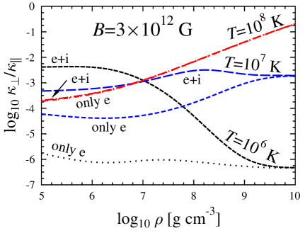
Figure 5: (color online) Anisotropy of the thermal conductivity $\kappa_{\perp}/\kappa_{\parallel}$ versus density for the magnetic field $B=3\times 10^{12}$ G and three values of the temperature $\log_{10}T[K]$=6.0, 7.0, and 8.0. See text for details.

A magnetic field introduces a considerable anisotropy in thermal conduction of the neutron star envelope. For illustration, in Fig. 5 we plot the density dependence of the anisotropy, which is the ratio of the transverse conductivity $\kappa_{\perp}=\kappa_{\mathrm{i}}+\kappa_{\mathrm{e\perp}}$ to the longitudinal conductivity $\kappa_{\parallel}=\kappa_{\mathrm{i}}+\kappa_{\mathrm{e\parallel}}\approx\kappa_{\mathrm{e\parallel}}$ of the matter. We take the same magnetic field $B=3\times 10^{12}$ G and the same three values of the temperature $\log_{10}T$=6, 7, and 8 K, as in Fig. 3. The lines marked ‘e+i’ are plotted taking into account both, electron and ion, conductivities. We see that the anisotropy can be very strong, and it increases with lowering $T$, when the star cools. For instance, we have $\kappa_{\perp}/\kappa_{\parallel}\sim 0.1$ for $T=10^{8}$ K and $\rho\sim 10^{8}$ g cm^-3 but $\kappa_{\perp}/\kappa_{\parallel}\sim 10^{-6}$ for $T=10^{6}$ K and the same $\rho\sim 10^{8}$ g cm^-3. To emphasize the importance of the ion conduction, the lines marked as ‘only e’ in Fig. 5 show the anisotropy $\kappa_{\mathrm{e\perp}}/\kappa_{\mathrm{e\parallel}}$ produced by electron conduction alone. At $T=10^{8}$ K the ion conductivity is small and does not affect heat transport as discussed above (curves ‘e+i’ and ‘only e’ merge). However, at lower $T$ ion conduction becomes important. It is clearly seen that $\kappa_{\mathrm{i}}$ greatly reduces the heat conduction anisotropy at sufficiently low $\rho$, where ion conduction dominates in the transverse heat transport (see Fig. 3 and the discussion above). For instance, taking $T=10^{6}$ K and $\rho=10^{6}$ g cm^-3 and neglecting the ion contribution, we would have a very strong heat transport anisotropy $\kappa_{\mathrm{e\perp}}/\kappa_{\mathrm{e\parallel}}\approx 10^{-6}$, while the inclusion of the ion conductivity gives $\kappa_{\mathrm{\perp}}/\kappa_{\mathrm{\parallel}}\sim 10^{-3}$. This means that the heat transport becomes much more isotropic (by approximately three orders of magnitude). This effect may strongly affect the temperature distribution in the neutron star heat blanketing envelope and over the surface, the relation between the internal neutron star temperature and surface thermal luminosity, and the neutron star cooling.

8 Conclusions

We have calculated the thermal conductivity of ions $\kappa_{\mathrm{i}}$ in large ranges of the density and temperature in a neutron star envelope. We have taken into account ion-ion and ion-electron scattering (equivalent to phonon-phonon and phonon-electron scattering at sufficiently low temperatures) and analyzed various ion-conduction regimes. We have performed extensive Monte Carlo calculations of $\kappa_{\mathrm{ie}}$ due to phonon-electron scattering. All our results are approximated by simple analytic expressions. In this way we have got a systematic description of all ion conduction regimes in neutron star envelopes. We have compared calculated values of $\kappa_{\mathrm{i}}$ with the values of the electron thermal conductivity $\kappa_{\mathrm{e}}$ which is usually the only thermal conductivity taken into account in neutron star envelopes (except for neutron star atmospheres, where heat transport is radiative).

Our main conclusions are:

1. The ion thermal conductivity is much less affected by neutron star magnetic fields than the electron thermal conductivity (and we have neglected the effects of magnetic fields on $\kappa_{\mathrm{i}}$).

2. The ion thermal conductivity is typically much lower than the electron thermal conductivity along magnetic field lines in the neutron star envelope. Heat conduction along the magnetic field lines is mostly provided by electrons.

3. The ion thermal conductivity can be higher than the electron thermal conductivity across magnetic field lines in the outer envelope of a neutron star at not too high temperatures and densities ($T\lesssim 10^{8}$ K and $\rho\lesssim 10^{9}$ g cm^-3 for $B\sim 3\times 10^{12}$ G).

4. The conductivity $\kappa_{\mathrm{i}}$ at low temperatures and high densities is determined by electron-ion collisions (e.g., at $\rho\gtrsim 3\times 10^{8}$ g cm^-3 for $T\sim 10^{7}$ K) although at lower $\rho$ and higher $T$ it is determined by ion-ion collisions.

5. The inclusion of $\kappa_{\mathrm{i}}$ can strongly (by a few orders of magnitude) reduce large anisotropy of thermal conduction in magnetized neutron star envelopes, affecting thus temperature distribution in the heat blanketing envelope and over the stellar surface, and cooling of magnetized neutron stars.

Our results extend those obtained by (Pérez-Azorín et al.2006). First, we have included the contribution of electron-phonon scattering. Second, we have improved the consideration of phonon-phonon scattering. Finally, we have analyzed different ion conduction regimes. Nevertheless, we stress that our results are semi-quantitative and can be elaborated further. In particular, it would be interesting to consider phonon scattering in impure and imperfect crystals (by studying phonon-impurity scattering neglected here), to take into account electron band structure effects in phonon-electron scattering, to describe accurately phonon-phonon scattering [without using the estimate Eq. (21)], and the effects of magnetic fields on the ion thermal conductivity. All these problems open a new and interesting field of neutron star kinetics which goes far beyond the scope of the present paper. We expect to deal with them in future publications.

References

- Abramowitz & Stegun (1972) Abramowitz M., Stegun I.A. (eds.), 1972, Handbook of Mathematical Functions, Dover, New York
- Baiko & Yakovlev (1995) Baiko D.A., Yakovlev D.G., 1995, Astron. Lett. 21, 702
- Baiko et al. (1998) Baiko D.A., Kaminker A.D., Potekhin A.Y., Yakovlev D.G., 1998, Phys. Rev. Lett., 81, 5556
- Baiko (2000) Baiko D.A., 2000, ”Kinetic phenomena in cooling neutron stars”, PhD thesis (Ioffe Phys.-Tech. Inst., St. Petersburg) [in Russian], unpublished
- Baiko et al. (2001) Baiko D.A., Potekhin A.Y., Yakovlev D.G., 2001, Phys. Rev. E, 64, 057402
- Baiko (2002) Baiko D.A., 2002, Phys. Rev. E, 66, 056405
- Bernu & Vieillefosse (1978) Bernu B., Vieillefosse P., 1978, Phys. Rev. A, 18, 2345
- Burwitz et al. (2003) Burwitz V., Haberl F., Neuhäuser R., Predehl P., Trümper J., Zavlin V.E., 2003, A & A, 399, 1109
- Braginski (1963) Braginski S.I., 1963, in Voprosy Teorii Plasmy, vol.1, ed. by M.A. Leontovich (GosAtomIzdat: Moscow); English translation: 1965, Reviews of Plasma Physics, vol.1, ed. by M.A. Leontovich, (Consultants Bureau: New York) p. 205
- Cohen & Keffer (1955) Cohen M.H., Keffer F., 1955, Phys. Rev., 99, 1128
- Daligault (2006) Daligault J., Phys. Rev. Lett., 96, 065003
- Dubin (1990) Dubin D.H.E., Phys. Rev. A, 42, 4972
- (13) Geppert U., Kueker M., Page D., 2004, A & A, 426, 267
- (14) Geppert U., Kueker M., Page D., 2006, A & A, 457, 937
- (15) Gnedin O.Y., Yakovlev D.G., Potekhin A.Y., 2001, MNRAS, 324, 725
- Flowers & Itoh (1976) Flowers E., Itoh N., 1976, ApJ, 206, 218
- Haberl (2007) Haberl F., Astrophys Space Sci., 308, 181
- (18) Haensel P., Potekhin A.Y., and Yakovlev D.G., 2007, Neutron Stars 1: Equation of State and Structure. Springer Verlag, New York
- Ho (2007) Ho W.C.G., 2007, MNRAS, 380, 71
- Landau & Lifshitz (1993) Landau L.D., Lifshitz E.M., 1993, Statistical Physics, Part 1. Pergamon, Oxford
- Lifshitz & Pitaevski (1980) Lifshitz E.M., Pitaevskiĭ L.P., 1980, Statistical Physics, Part 2. Pergamon, Oxford
- McGaughey & Kaviany (2006) McGaughey A.J.H., Kaviany M., 2006, Advances in Heat Transfer, 39, 169
- Negele & Vautherin (1973) Negele J.W., Vautherin D., 1973, Nucl. Phys. A, 207, 298
- Oyamatsu (1993) Oyamatsu K., Nucl. Phys. A, 561, 431
- Raikh & Yakovlev (1982) Raikh M.E., Yakovlev D.G., 1982, Astrophys. Sp. Sci., 87, 193
- (26) Page D., Geppert U., Weber F., 2006, Nucl. Phys. A 777, 497
- (27) Pérez-Azorín J.F., Miralles J.A., Pons J.A., 2006, A&A, 451, 1009.
- Pethick & Thorsson (1997) Pethick C.J., Thorsson V., 1997, Phys. Rev. D, 56, 7548
- (29) Pierleoni C., Ciccotti G., Bernu B., 1987, Europhysics Letters, 4, 1115
- (30) Potekhin A.Y., Chabrier G., Yakovlev D.G., 1997, A&A 323, 415
- Potekhin (1999) Potekhin A.Y., 1999, A&A, 351, 787
- Potekhin et al. (1999) Potekhin A.Y., Baiko D.A., Haensel P., Yakovlev D.G., 1999, A&A, 346, 345.
- Pollock & Hansen (1973) Pollock L.E., Hansen J.P., 1973, Phys. Rev. A, 8, 3110
- Schmidt et al. (1997) Schmidt P., Zwicknagel G., Reinhardt P.G., Toepffer C., 1997, Phys. Rev. E, 56, 7310
- Shternin & Yakovlev (2006) Shternin P.S., Yakovlev D.G., 2006, Phys. Rev. D, 74, 043004
- Ventura & Potekhin (2001) Ventura J., Potekhin A.Y., 2001, in The Neutron Star – Black Hole Connection, NATO Science Ser. C, 567, edited by C. Kouveliotou, E.P.J. van den Heuvel, & J. Ventura (Kluwer, Dordrecht), 393
- Yakovlev & Kaminker (1994) Yakovlev D.G., Kaminker A.D., 1994 in The Equation of State in Astrophysics, edited by G. Chabrier & E. Schatzman (Cambridge University Press, Cambridge), 214
- Ziman (1960) Ziman J.M., 1960, Electrons and Phonons. Oxford Univ. press, Oxford