One-loop corrections to the mass
of self-dual semi-local planar
topological solitons

Abstract

A formula is derived that allows the computation of one-loop mass shifts for self-dual semilocal topological solitons. These extended objects, which in three spatial dimensions are called semi-local strings, arise in a generalized Abelian Higgs model with a doublet of complex Higgs fields. Having a mixture of global, $SU(2)$, and local (gauge), $U(1)$, symmetries, this weird system may seem bizarre, but it is in fact the bosonic sector of electro-weak theory when the weak mixing angle is ${\pi\over 2}$. The procedure for computing the semi-classical mass shifts is based on canonical quantization and heat kernel/zeta function regularization methods.

PACS: 03.70.+k;11.15.Kc;11.15.Ex

Keywords: Semi-local topological solitons; Heat-kernel/Zeta function regularization; One-loop shifts to soliton masses

1 Introduction

The purpose of this paper is to address the computation and analysis of one-loop shifts to the masses of semi-local planar topological solitons arising in a natural generalization of the Abelian Higgs model. Seen in (3+1)-dimensional space-time these solitons become semi-local strings whereas their masses give the string tensions, see [1]-[2]. At the critical point that marks the phase transition between Type I and Type II superconductivity, the set of semi-local self-dual topological solitons is an interesting $4l$-dimensional moduli space, where $l$ is the number of quanta of the magnetic flux, see [3]-[4]. Recently, superconducting semilocal (non self-dual) strings with very intriguing properties have been discovered in this model [5].

Computations of one-loop mass corrections will be performed using the heat kernel/zeta function regularization method. The high-temperature asymptotic expansion of the heat function, see [7]-[6]-[8]-[9], is a powerful tool that was applied for the first time to the calculation of kink mass shifts in [10] -the ${\cal N}=1$ SUSY case- and [11] -the non SUSY case-. One-loop corrections to ${\cal N}=2$ supersymmetric self-dual Nielsen-Olesen vortices were computed in a similar approach by Vassilevich and Rebhan-van Nieuwenhuizen-Wimmer in References [12] and [13]. In the second paper, the authors also showed that the central charge of the SUSY algebra is modified in one-loop order in such a way that the Bogomolny bound is saturated at the semi-classical level. Sometime later, we calculated the one-loop mass shift for ${\cal N}=0$ (non-SUSY) self-dual NO vortices carrying a quantum of magnetic flux in Reference [15]. Mass shifts have been given for spherically symmetric self-dual vortices (when several solitons of a quantum of flux have coinciding centers) in [16] up to four magnetic flux quanta. Cruder approximations were also provided for the mass shift of two separated self-dual NO vortices -each of them with a quantum of magnetic flux- as a function of the inter-center distance.

In Reference [17], we studied the one-loop correction to the energy of a degenerate manifold of kinks that arise in a very interesting family of models with two real scalar fields in (1+1)-dimensions. These field theoretical systems are obtained through dimensional reduction -plus a reality condition- of an ${\cal N}=1$ supersymmetric Wess-Zumino model with two chiral super-fields, see [18]-[19]-[20]. A comparison between the mass shifts of these composite kinks and the correction to the mass of the ordinary $\lambda\phi_{2}^{4}$ kink was offered in [21]. In this paper, we address a similar, but more difficult, situation in (2+1)-dimensions, comparing one-loop mass corrections of the topological solitons that arise in two planar Abelian gauge systems; one with two complex scalar fields and the other with a single complex scalar field. The methodology used to accomplish this task is explained in detail in Reference [22], where a complete list of References can be found.

Our paper is organized as follows: in Section §2 we describe the model and develop perturbation theory around one of the vacua. A one-loop renormalization is also performed. Section §3 is devoted to summarizing the structure of the moduli space of self-dual topological solitons. As a novelty, we also apply a variation of the de Vega-Shaposnik method [23] to find numerical solutions for spherically symmetric topological solitons. In Section §4, we explain how to obtain one-loop mass shifts in terms of generalized zeta functions of the second-order differential operators ruling the small fluctuations of the bosonic and ghost fields, and in §5 the high-temperature expansion of the heat kernel is used to give the final formula for one-loop mass shifts of semi-local self-dual topological solitons after application of Mellin’s transforms. We present our results in Section §6 by means of Mathematica calculations of the coefficients of the asymptotic series giving the heat functions. Finally, in the Appendix we offer several Tables where these coefficients are shown.

2 The planar semilocal Abelian Higgs model

The Model

The semi-local Abelian Higgs model [1] describes the minimal coupling between an $U(1)$-gauge field $A_{\mu}$ and a doublet $\Phi$ of complex scalar fields in a phase where the Higgs mechanism takes place. The term semilocal refers to the fact that while the global symmetry of this system is $SU(2)\times U(1)$ only the $U(1)$ factor is gauged. Defining non-dimensional space-time variables, $x^{\mu}\rightarrow\frac{1}{ev}x^{\mu}$, and fields, $\Phi\rightarrow v\Phi$, $A_{\mu}\rightarrow vA_{\mu}$, from the vacuum expectation value of the Higgs field $v$ and the $U(1)$-gauge coupling constant, $e$, the action for the semilocal Abelian Higgs model in (2+1)-dimensions reads:

$$S=\frac{v}{e}\int d^{3}x\left[-\frac{1}{4}F_{\mu\nu}F^{\mu\nu}+\frac{1}{2}(D_{\mu}\Phi)^{\dagger}D^{\mu}\Phi-\frac{\kappa^{2}}{8}(\Phi^{\dagger}\Phi(x^{\mu})-1)^{2}\right]\qquad,$$

where the covariant derivative is defined as $D_{\mu}\Phi=(\frac{\partial}{\partial x^{\mu}}-iA_{\mu})\Phi$. The physical spectrum differs from that of the standard AHM model in that, along with the massive vector boson and Higgs scalar, there is a complex Goldstone field. The parameter $\kappa^{2}=\frac{\lambda}{e^{2}}$ measures the ratio between the square of the masses of the Higgs, $M^{2}=\lambda v^{2}$, and vector particles, $m^{2}=e^{2}v^{2}$. Here, $\lambda$ is the Higgs field self-coupling. We choose a system of units where $c=1$, but $\hbar$ has dimensions of length $\times$ mass.

Feynman Rules in the Feynman-’t Hooft R gauge

In order to obtain the Feynman rules, we expand the action around a classical vacuum. We shall profit from the $SU(2)$ global invariance and we choose a vacuum $\Phi^{V}$ with real upper and vanishing lower components. The shift of the fields

$$\Phi(x^{\mu})=\left(\begin{array}[]{c}1+H(x^{\mu})+iG(x^{\mu})\\ \sqrt{2}\varphi(x^{\mu})\end{array}\right)$$

corresponds to the identification of $H(x^{\mu})$, $G(x^{\mu})$, and $\varphi(x^{\mu})$, respectively as Higgs, real, and complex Goldstone fields. The choice of the Feynman-’t Hooft R-gauge

$$R(A_{\mu},G)=\partial_{\mu}A^{\mu}+G$$

requires a Faddeev-Popov determinant to restore unitarity, which amounts to introducing a complex ghost field $\chi$. All this together allows us to write the action in the form

$$S = {v\over e}\int\,d^{3}x\,\left[-\frac{1}{2}A_{\mu}[-g^{\mu\nu}(\Box+1)]A_{\nu}+\partial_{\mu}\chi^{*}\partial^{\mu}\chi-\chi^{*}\chi\right.$$

$$+ \frac{1}{2}\partial_{\mu}G\partial^{\mu}G-\frac{1}{2}G^{2}+\frac{1}{2}\partial_{\mu}H\partial^{\mu}H-\frac{\kappa^{2}}{2}H^{2}+\partial_{\mu}\varphi^{*}\partial^{\mu}\varphi$$

$$- {\kappa^{2}\over 2}H(H^{2}+G^{2})+A_{\mu}(\partial^{\mu}HG-\partial^{\mu}GH)+H(A_{\mu}A^{\mu}-\chi^{*}\chi)+iA_{\mu}(\varphi^{*}\partial^{\mu}\varphi-\varphi\partial^{\mu}\varphi^{*})$$

$$+ \left.A_{\mu}A^{\mu}|\varphi|^{2}-\frac{\kappa^{2}}{8}(H^{2}+G^{2})^{2}+\frac{1}{2}(G^{2}+H^{2})A_{\mu}A^{\mu}-\frac{\kappa^{2}}{2}|\varphi|^{2}(|\varphi|^{2}+H^{2}+G^{2}+2H)\right]$$

in order to deduce the Feynman rules for the propagators and vertices shown in Tables 1 and 2. The propagator of the complex Goldstone boson plus two trivalent and four tetravalent vertices accounting for the interactions of Goldstone-anti-Goldstone pairs must be added to the Feynman rules of the Abelian Higgs model in the Feynman-’t Hooft gauge. Nevertheless, in order to guarantee that all physical quantities will be ultraviolet finite there is still a remaining piece to be added: the action for the counter-terms. We shall compute this up to one-loop order in the sequel.

Table 1: Propagators

Particle	Field	Propagator	Diagram
Higgs	$H(x)$	$\displaystyle\frac{ie\hbar}{v(k^{2}-\kappa^{2}+i\varepsilon)}$
Real Goldstone	$G(x)$	$\displaystyle\frac{ie\hbar}{v(k^{2}-1+i\varepsilon)}$
Complex Goldstone	$\varphi(x)$	$\displaystyle\frac{ie\hbar}{v(k^{2}+i\varepsilon)}$
Ghost	$\chi(x)$	$\displaystyle\frac{ie\hbar}{v(k^{2}-1+i\varepsilon)}$
Vector Boson	$A_{\mu}(x)$	$\frac{-ie\hbar g^{\mu\nu}}{v(k^{2}-1+i\varepsilon)}$

Table 2: Third- and fourth-order vertices

Vertex	Weight	Vertex	Weight	Vertex	Weight	Vertex	Weight
	$-3i\kappa^{2}\frac{v}{\hbar e}$		$-3i\kappa^{2}\frac{v}{\hbar e}$		$i(k^{\mu}+q^{\mu})\frac{v}{\hbar e}$		$2ig^{\mu\nu}\frac{v}{\hbar e}$
	$-i\kappa^{2}\frac{v}{\hbar e}$		$-3i\kappa^{2}\frac{v}{\hbar e}$		$(k^{\mu}-q^{\mu})\frac{v}{\hbar e}$		$2i\frac{v}{\hbar e}g^{\mu\nu}$
	$2i\frac{v}{\hbar e}g^{\mu\nu}$		$-i\kappa^{2}\frac{v}{\hbar e}$		$-2i\kappa^{2}\frac{v}{\hbar e}$		$-i\kappa^{2}\frac{v}{\hbar e}$
	$-i\frac{v}{\hbar e}$		$2i\frac{v}{\hbar e}g^{\mu\nu}$		$-i\kappa^{2}\frac{v}{\hbar e}$		$-i\kappa^{2}\frac{v}{\hbar e}$

One-loop mass renormalization counter-terms

All ultraviolet divergences come from the integral:

$$I(c^{2})=\int\,\frac{d^{3}k}{(2\pi)^{3}}\cdot\frac{i}{k^{2}-c^{2}+i\varepsilon}\qquad.$$

We also note that even if there are massless particles propagating in 2+1 dimensions, $I(0)$ is infrared convergent. The renormalization of the semilocal AHM requires the computation of the following one-loop graphs:

1. Higgs boson tadpole:

   $+$ $+$ $+$ $+$ $=$

   $$=-2i(\kappa^{2}+1)\cdot\,I(1)-i\kappa^{2}\cdot\,I(0)+\mbox{finite part}$$

2. Higgs boson self-energy:

   $+$ $+$ $+$ $+$ $=$

   $$=-2i(\kappa^{2}+1)\cdot\,I(1)-i\kappa^{2}\cdot\,I(0)+\mbox{finite part}$$

3. Real Goldstone boson self-energy:

   $+$ $+$ $+$ $+$ $=$

   $$=-2i(\kappa^{2}+1)\cdot\,I(1)-i\kappa^{2}\cdot\,I(0)+\mbox{finite part}$$

4. Complex Goldstone boson self-energy:

   $+$ $+$ $+$ $+$   $=$

   $$=-4i(\kappa^{2}+1)\cdot\,I(1)-2i\kappa^{2}\cdot\,I(0)+\mbox{finite part}$$

5. Vector boson self-energy: The potentially divergent part is

   $+$ $+$ $+$ $+$

   $$=2i\cdot\,[I(1)+I(0)]g^{\mu\nu}+\mbox{finite part}\qquad.$$

In (2+1)-dimensions the graphs above are the only ultraviolet divergent diagrams for any number of loops in the diagrams, not only in one-loop order, and the theory is super-renormalizable. Thus, in a minimal subtraction scheme we get rid off all ultraviolet divergences arising in the vacuum sector of the model by adding the counter-terms

$${\cal L}_{c.t.}^{S} = {\hbar\over 2}\left[2(\kappa^{2}+1)\cdot\,I(1)+\kappa^{2}\cdot\,I(0)\right]\cdot\,\left[\Phi^{*}_{1}(x^{\mu})\Phi_{1}(x^{\mu})+\Phi^{*}_{2}(x^{\mu})\Phi_{2}(x^{\mu})-1\right]$$

$${\cal L}_{c.t.}^{A} = -\hbar[I(1)+I(0)]\cdot\,A_{\mu}(x^{\mu})A^{\mu}(x^{\mu})$$

Table 3: Counter-term vertices

Diagram		Weight
		$\displaystyle i[2(\kappa^{2}+1)I(1)+\kappa^{2}I(0)]$
		$\displaystyle i[2(\kappa^{2}+1)I(1)+\kappa^{2}I(0)]$
		$\displaystyle i[2(\kappa^{2}+1)I(1)+\kappa^{2}I(0)]$
		$\displaystyle i[4(\kappa^{2}+1)I(1)+2\kappa^{2}I(0)]$
		$\displaystyle-2i[I(1)+I(0)]g^{\mu\nu}$

,

which gives rise to the vertices shown in Table 3. In our renormalization scheme, finite renormalizations have been adjusted in such a way that, on one hand, the divergence due to the tadpole graph is exactly canceled when the theory is fine-tuned to the so called self-dual limit $\kappa^{2}=1$ and, on the other hand, the global $SU(2)$ symmetry remains unbroken up to one-loop order.

3 Semilocal vortices

Finite energy solutions

Apart from the ground states built around the $S^{3}$ classical homogeneous solutions, the semilocal AHM has room for other quantum states arising from the extended classical configurations, which are stable owing to topological reasons. These configurations are the topological solitons that appear at tree level as non-homogeneous solutions of the static field equations:

$$\partial_{i}F_{ij}=\frac{i}{2}\left(\Phi^{\dagger}D_{j}\Phi-(D_{j}\Phi)^{\dagger}\right)\qquad,\qquad D_{i}D_{i}\Phi=\frac{\kappa^{2}}{4}\Phi(\Phi^{\dagger}\Phi-1)\qquad,$$

such that their energy,

$$E=\int d^{2}x[\frac{1}{4}F_{ij}F_{ij}+\frac{1}{2}(D_{i}\Phi)^{\dagger}D_{i}\Phi+\frac{\kappa^{2}}{8}(\Phi^{\dagger}\Phi-1)^{2}]\qquad,$$

is finite. The topological character of these solutions is peculiar in that although the scalar vacuum manifold is $S^{3}$, and thus simply connected, the configuration space ${\cal C}$

$${\cal C}=\left\{\Phi(\vec{x})\in Maps({\mathbb{R}}^{2},{\mathbb{C}}^{2}),A_{i}(\vec{x})\in Maps({\mathbb{R}}^{2},T{\mathbb{R}}^{2})/E(\Phi,A_{i})<+\infty\right\}$$

is the union of ${\mathbb{Z}}$ disconnected sectors. Finite energy configurations show the asymptotic behavior

$$\Phi^{\dagger}\Phi|_{S_{\infty}^{1}}=1\hskip 56.9055pt,\hskip 56.9055ptD_{i}\Phi|_{S_{\infty}^{1}}=(\partial_{i}\Phi-iA_{i}\Phi)|_{S_{\infty}^{1}}=0,$$

where $S_{\infty}^{1}$ is the circle that bounds the plane at infinity. Parametrizing $S^{1}_{\infty}$ by the polar angle $\theta={\rm arctan}\frac{x_{2}}{x_{1}}$, and, modulo the global $SU(2)$-symmetry, choosing $\Phi|_{S_{\infty}^{1}}=\Phi^{V}$ for $\theta=0$, the boundary conditions on the covariant derivatives provide a map, $S^{1}_{\infty}\longrightarrow S^{1}_{1}$, between the sphere at the infinity spatial and the fiber $S_{1}^{1}$ at the north pole of the base $S^{2}$ of the $S^{3}$ vacuum Hopf bundle:

$$\Phi|_{S_{\infty}^{1}}=\left(\begin{array}[]{c}\Phi_{1}|_{S_{\infty}^{1}}\\ \Phi_{2}|_{S_{\infty}^{1}}\end{array}\right)=\left(\begin{array}[]{c}\phi_{1}|_{S_{\infty}^{1}}+i\phi_{2}|_{S_{\infty}^{1}}\\ \phi_{3}|_{S_{\infty}^{1}}+i\phi_{4}|_{S_{\infty}^{1}}\end{array}\right)=\left(\begin{array}[]{c}e^{il\theta}\\ 0\end{array}\right)\,\,\qquad,\,\,\qquad l\in{\mathbb{Z}}\qquad.$$

Continuous maps between one-dimensional spheres are classified according to the first homotopy group and, because the temporal evolution is continuous, $\Pi_{0}({\cal C})=\Pi_{1}(S^{1}_{1})={\mathbb{Z}}$, the zero homotopy group of ${\cal C}$ is non-trivial. Thus, ${\cal C}=\sqcup_{l\in{\mathbb{Z}}}{\cal C}_{l}$ is the union of disconnected sectors characterized by an integer number $l$.

Moreover, the boundary condition for the vector field $A_{i}|_{S_{\infty}^{1}}=-i\Phi^{\dagger}\partial_{i}\Phi|_{S_{\infty}^{1}}$ is tantamount to:

$$A_{i}(\vec{x})\left|{}_{S^{1}_{\infty}}\right.=\phi_{1}(\vec{x})\frac{\partial\phi_{2}}{\partial x_{i}}(\vec{x})\left|{}_{S^{1}_{\infty}}\right.-\phi_{2}(\vec{x})\frac{\partial\phi_{1}}{\partial x_{i}}(\vec{x})\left|{}_{S^{1}_{\infty}}\right.+\phi_{3}(\vec{x})\frac{\partial\phi_{4}}{\partial x_{i}}(\vec{x})\left|{}_{S^{1}_{\infty}}\right.-\phi_{4}(\vec{x})\frac{\partial\phi_{3}}{\partial x_{i}}(\vec{x})\left|{}_{S^{1}_{\infty}}\right.$$

The $SU(2)$-orbit of $\Phi_{l}^{V}=\left(\begin{array}[]{c}e^{il\theta}\\ 0\end{array}\right)$ is:

$$G\Phi_{l}^{V}=\left(\begin{array}[]{cc}e^{i\theta_{1}}{\rm sin}\psi&e^{i\theta_{2}}{\rm cos}\psi\\ -e^{-i\theta_{2}}{\rm cos}\psi&e^{-i\theta_{1}}{\rm sin}\psi\end{array}\right)\left(\begin{array}[]{c}e^{il\theta}\\ 0\end{array}\right)=\left(\begin{array}[]{c}e^{i(\theta_{1}+l\theta)}{\rm sin}\psi\\ -e^{-i(\theta_{2}-l\theta)}{\rm cos}\psi\end{array}\right)\qquad,$$

where $\theta_{1},\theta_{2}\in[0,2\pi]$ and $\psi\in[0,{\pi\over 2}]$ are the Hopf coordinates of the $S^{3}$ sphere. Therefore,

$$A_{i}(\vec{x})\left|{}_{S^{1}_{\infty}}\right. = l\frac{\partial\theta}{\partial x_{i}}\left({\rm cos}^{2}(\theta_{1}+l\theta){\rm sin}^{2}\psi+{\rm sin}^{2}(\theta_{1}+l\theta){\rm sin}^{2}\psi\right)+$$

$$+ l\frac{\partial\theta}{\partial x_{i}}\left({\rm cos}^{2}(\theta_{2}-l\theta){\rm cos}^{2}\psi+{\rm sin}^{2}(\theta_{2}-l\theta){\rm cos}^{2}\psi\right)$$

$$= l\frac{\partial\theta}{\partial x_{i}}$$

and the topological (winding) number $l$ has a direct physical interpretation in terms of the magnetic flux carried by the planar soliton:

$$g=\oint_{S^{1}_{\infty}}\,\left(A_{1}(\vec{x})dx^{1}+A_{2}(\vec{x})dx^{2}\right)=l\oint\,\left(\frac{\partial\theta}{\partial x_{1}}dx^{1}+\frac{\partial\theta}{\partial x_{2}}dx^{2}\right)=l\int_{0}^{2\pi}\,d\theta=2\pi l\qquad.$$

Self-dual semi-local topological solitons

We shall restrict ourselves to the critical point between Type I and Type II superconductivity: $\kappa^{2}=1$. The energy can be arranged in a Bogomolny splitting:

$$E=\int\frac{d^{2}x}{2}\left((D_{1}\Phi\pm iD_{2}\Phi)^{\dagger}(D_{1}\Phi\pm iD_{2}\Phi)+[F_{12}\pm{\textstyle\frac{1}{2}}(\Phi^{\dagger}\Phi-1)]^{2}\right)+\frac{1}{2}|g|$$

One immediately realizes that the solutions of the first-order equations

$$D_{1}\Phi\pm iD_{2}\Phi=0\hskip 42.67912pt,\hskip 42.67912ptF_{12}\pm\frac{1}{2}(\Phi^{\dagger}\Phi-1)=0$$ (1)

are absolute minima of the energy, and are hence stable, in each topological sector that has a classical mass proportional to the magnetic flux. Because the first-order equations can be obtained from the self-duality equations of Euclidean 4D gauge theory through dimensional reduction, the vortex solutions of (1) are called self-dual at the limit $\kappa^{2}=1$.

We follow [3] to summarize the properties and existence of the so-called semi-local self-dual topological solitons: the solutions of (1) for non-negative $l$ (plus sign in the first-order equations). The equation on the left in (1) is tantamount to:

$$\bar{A}(z,\bar{z})=-i\partial_{\bar{z}}\,\log\,\Phi_{a}(z,\bar{z})\quad,\quad a=1,2\qquad\qquad,\qquad\Phi(z,\bar{z})=\left(\begin{array}[]{c}\Phi_{1}(z,\bar{z})\\ \Phi_{2}(z,\bar{z})\end{array}\right)\qquad,$$ (2)

where the complex notation for coordinates and fields is:

$$z=x_{1}+ix_{2}\qquad,\qquad\partial_{z}={1\over 2}(\partial_{1}-i\partial_{2})\qquad,\qquad A={1\over 2}(A_{1}-iA_{2})\qquad.$$

From (2), one sees that:

$$\partial_{\bar{z}}\,\log\left(\frac{\Phi_{2}(z,\bar{z})}{\Phi_{1}(z,\bar{z})}\right)=0\qquad\Longrightarrow\qquad\omega(z)=\frac{\Phi_{2}(z,\bar{z})}{\Phi_{1}(z,\bar{z})}=\frac{Q_{m}(z)}{P_{l}(z)}$$

where $Q_{m}$ and $P_{l}$ are polynomials of respective degree $m$ and $l$ in $z$, such that $\omega(z)$ is locally analytic. The behavior of the Higgs field at infinity (up to global $SU(2)$ transformations) compatible with finite energy requires that $m<l$ and $P_{l}(z)$ be monic:

$$P_{l}(z)=z^{l}+p_{l-1}z^{l-1}+\cdots+p_{1}z+p_{0}\qquad,\qquad Q_{l-1}(z)=q_{l-1}z^{l-1}+\cdots+q_{1}z+q_{0}\qquad.$$

Therefore, the moduli space of semi-local topological solitons depends on $2l$ complex ($4l$ real) parameters: $(p_{a},q_{a}),a=0,1,\cdots,l-1$. Varying the values of $(p_{a},q_{a})$ one varies the $l$ zeroes of $\Phi_{1}$ and the $l-1$ zeroes of $\Phi_{2}$ in such a way that the locations of the zeroes of the two Higgs fields plus the scale and orientation of $\Phi_{2}$ parametrize the SSTS moduli space. Equation (1) on the right becomes

$$\bigtriangleup\,u(z,\bar{z})+1-e^{u(z,\bar{z})}=\bigtriangleup\,\log\,\left(\left|P_{l}\right|^{2}(z)+\left|Q_{l-1}\right|^{2}(z)\right)\qquad,$$ (3)

where

$$u(z,\bar{z})=\Omega(z,\bar{z})+\log\,(1+|\omega|^{2}(z))\qquad,\qquad\Omega(z,\bar{z})=\log\,\Phi_{1}^{*}\Phi_{1}(z,\bar{z})\qquad.$$

By functional analysis techniques, it is possible to demonstrate the existence and uniqueness of a solution of (3) compatible with finite energy boundary conditions [3, 4]. Therefore, the finite energy solutions of (1) with a magnetic flux $2\pi l$ take the form

$$\left(\begin{array}[]{c}\Phi_{1}^{(l)}(z,\bar{z})\\ \Phi_{2}^{(l)}(z,\bar{z})\end{array}\right)=\frac{1}{\sqrt{\left|P_{l}\right|^{2}(z)+\left|Q_{l-1}\right|^{2}(z)}}\cdot\left(\begin{array}[]{c}P_{l}(z)\\ Q_{l-1}(z)\end{array}\right)\cdot e^{{1\over 2}u(z,\bar{z})}\qquad,$$

where $u(z,\bar{z})$ is a solution of (3). In the $l=1$ case we have that:

$$\left(\begin{array}[]{c}\Phi_{1}^{(l=1)}(z,\bar{z};q_{0})\\ \Phi_{2}^{(l=1)}(z,\bar{z};q_{0})\end{array}\right)=\frac{1}{\sqrt{\left|z-z_{0}\right|^{2}+\left|q_{0}\right|^{2}}}\cdot\left(\begin{array}[]{c}z-z_{0}\\ q_{0}\end{array}\right)\cdot e^{{1\over 2}u(|z-z_{0}|;\,\,q_{0})}\qquad.$$

Setting the parameter $q_{0}$ to zero, we find the embedded Nielsen-Olesen vortex centered at $z_{0}$:

$$\left(\begin{array}[]{c}\Phi_{1}^{(l=1)}(z,\bar{z};0)\\ \Phi_{2}^{(l=1)}(z,\bar{z};0)\end{array}\right)=\left(\begin{array}[]{c}\frac{z-z_{0}}{|z-z_{0}|}\\ 0\end{array}\right)\cdot e^{{1\over 2}u(|z-z_{0}|;\,\,0)}\qquad.$$

$$\bigtriangleup\log[|z-z_{0}|^{2}+|q_{0}|^{2}]=\frac{4|q_{0}|^{2}}{(|z-z_{0}|^{2}+|q_{0}|^{2})^{2}}\qquad,$$

however, tends to zero for very large $|q_{0}|$ and the solution of (3) becomes: $u(|z-z_{0}|;|q_{0}|>>1)\simeq 0$. Therefore,

$$\left(\begin{array}[]{c}\Phi_{1}^{(l=1)}(z,\bar{z};|q_{0}|>>1)\\ \Phi_{2}^{(l=1)}(z,\bar{z};|q_{0}|>>1)\end{array}\right)=\frac{1}{\sqrt{\left|z-z_{0}\right|^{2}+\left|q_{0}\right|^{2}}}\cdot\left(\begin{array}[]{c}z-z_{0}\\ q_{0}\end{array}\right)$$

is precisely the field profile of the lump centered at $z_{0}$ with radius $|q_{0}|$ and topological charge 1 in the planar ${\rm CP}^{1}$ model. The Higgs fields spreads over the vacuum manifold $S^{3}$ for very large $|q_{0}|$ whereas the ANO profiles are found for very small $|q_{0}|$. Self-dual semi-local topological solitons interpolate between self-dual ANO vortices and ${\rm CP}^{1}$-lumps when $|q_{0}|$ varies between 0 and $\infty$.

Self-dual semi-local topological solitons with spherical symmetry

Among the topological solitons, the simplest ones are those in which all the roots of both $P_{l}(z)=(z-z_{0})^{l}$ and $Q_{m}(z)=q_{m}(z-z_{0})^{m}$ are at the same point. Let us focus on this case by considering the spherically symmetric ansatz around this point chosen at the origin. If $r=+\sqrt{x_{1}^{2}+x_{2}^{2}}$, for configurations of the form

$$\Phi(x_{1},x_{2})=\left(\begin{array}[]{c}f(r)e^{il\theta}\\ |h(r)|e^{i(\lambda+m\theta)}\end{array}\right)\quad,\quad f(r)=\frac{r^{(l-m)}}{\sqrt{r^{2(l-m)}+|q_{m}|^{2}}}\cdot e^{{1\over 2}u(r;\,\,q_{m})}$$

$$A_{i}(x_{1},x_{2})=-l\varepsilon_{ij}\frac{\alpha(r)}{r^{2}}x_{j}\qquad,\qquad h(r)=\frac{q_{m}}{\sqrt{r^{2(l-m)}+|q_{m}|^{2}}}\cdot e^{{1\over 2}u(r;\,\,q_{m})}\qquad,$$

the first-order PDE’s reduce to a system of nonlinear ordinary differential equations:

$${1\over r}{d\alpha\over dr} = -\frac{1}{2l}(f^{2}(r)+|h(r)|^{2}-1)$$ (4)

$${df\over dr} = \frac{l}{r}f(r)[1-\alpha(r)]$$ (5)

$${d|h|\over dr} = {l\over r}|h|(r)({m\over l}-\alpha(r))$$ (6)

to be solved together with the boundary conditions

$${\displaystyle\lim_{r\rightarrow\infty}}f(r)=1\hskip 28.45274pt,\hskip 28.45274pt{\displaystyle\lim_{r\rightarrow\infty}}h(r)=0\hskip 28.45274pt,\hskip 28.45274pt{\displaystyle\lim_{r\rightarrow\infty}}\alpha(r)=1$$

$$f(0)=0\hskip 42.67912pt,\hskip 36.98866pt|h(0)|=|h_{0}|\delta_{m,0}\hskip 17.07182pt,\hskip 22.76228pt\alpha(0)=0$$ (7)

required by energy finiteness plus regularity at the center of the vortex. Let us recall that the boundary conditions at infinity also require that $m{\rm be}<l$. The magnetic field and the energy density of the spherically symmetric vortices in terms of the field profiles $f(r)$, $\alpha(r)$ are:

$$B(r)={l\over 2r}\frac{d\alpha}{dr}$$

$${\cal E}(r)={1\over 8}({1\over l^{2}}+1)(1-f^{2}(r)-|h(r)|^{2})^{2}+{l^{2}f^{2}(r)\over r^{2}}(1-\alpha(r))^{2}+\frac{l^{2}|h(r)|^{2}}{r^{2}}({m\over l}-\alpha(r))^{2}\qquad.$$

Semi-local strings with a quantum of magnetic flux

We now go on to the most elementary solutions that carry a quantum of magnetic flux, or, $l=1=m+1$ . We follow the procedure developed in [23] to solve the non-linear ODE system (4)-(5)-(6) with boundary conditions (7). First, we consider small values of $r$ and in the first-order differential equations we test the power series

$$f(r) \equiv f_{1}\cdot r+f_{2}\cdot r^{2}+f_{3}\cdot r^{3}+f_{4}r^{4}+\cdots$$ (8)

$$\alpha(r) \equiv \alpha_{1}\cdot r+\alpha_{2}\cdot r^{2}+\alpha_{3}\cdot r^{3}+\alpha_{4}\cdot r^{4}+\cdots$$ (9)

$$h(r) \equiv h_{0}+h_{1}\cdot r+h_{2}\cdot r^{2}+h_{3}\cdot r^{3}+h_{4}\cdot r^{4}+\cdots\qquad,$$ (10)

where $f_{j}$ and $\alpha_{j}$, $j=1,2,3,\cdots$, are real, whereas $h_{j}$, $j=0,1,2,\cdots$, are complex coefficients. The coupled first-order ODE’s are solved at this limit by (8)-(9)-(10) if

$$f(r) \simeq f_{1}\cdot r+\frac{f_{1}}{8}(|h_{0}|^{2}-1)\cdot r^{3}+\frac{f_{1}}{128}\left[(|h_{0}|^{2}-1)(2|h_{0}|^{2}-1)+4f_{1}^{2}\right]\cdot r^{5}+\dots$$

$$\alpha(r) \simeq \frac{1}{4}(1-|h_{0}|^{2})\cdot r^{2}-\left[\frac{1}{32}|h_{0}|^{2}(|h_{0}|^{2}-1)+\frac{1}{8}f_{1}^{2}\right]\cdot r^{4}-$$

$$- \left[\frac{1}{768}|h_{0}|^{2}(|h_{0}|^{2}-1)(3|h_{0}|^{2}-2)+\frac{1}{192}f_{1}^{2}(5|h_{0}|^{2}-4)\right]\cdot r^{6}+\dots$$

$$h(r) \simeq h_{0}+\frac{h_{0}}{8}(|h_{0}|^{2}-1)\cdot r^{2}+\frac{h_{0}}{128}\left[(|h_{0}|^{2}-1)(2|h_{0}|^{2}-1)+4f_{1}^{2}\right]\cdot r^{4}+\dots\qquad.$$

We stress that

$$h_{0}=\frac{q_{0}}{|q_{0}|}\cdot e^{{1\over 2}u(0;\,\,q_{0})}$$

is determined by the behavior of the solution at the origin. After that, only a free parameter, $f_{1}$, is left in the exact solution near the origin. Second, a numerical scheme is implemented by setting a boundary condition at a non-singular point of the ODE system, which is obtained from the power series for a small value of $r$ ($r=0.001$ in our case). This scheme prompts a shooting procedure by varying $f_{1}$, where the correct asymptotic behavior of the solutions is obtained by setting an optimal value for $f_{1}$ for a given value of $h_{0}$. Finally, the first-order ODE system is solved for large $r$ by means of a power series in ${1\over r}$:

$$f(r)=\sum_{j=0}f^{j}\cdot r^{-j}\hskip 14.22636pt,\hskip 14.22636pt\alpha(r)=\sum_{j=0}\alpha^{j}\cdot r^{-j}\hskip 14.22636pt,\hskip 14.22636pth(r)=\sum_{j=1}h^{j}\cdot r^{-j}\quad\qquad,$$

with the result that

$$f(r) \simeq 1-\frac{|h^{1}|^{2}}{2}\cdot r^{-2}+(-2|h^{1}|^{2}+\frac{3}{8}|h^{1}|^{4})\cdot r^{-4}+|h^{1}|^{2}(-32+5|h^{1}|^{2}-\frac{5}{16}|h^{1}|^{4})\cdot r^{-6}+$$

$$+ |h^{1}|^{2}(-1152+158|h^{1}|^{2}-\frac{35}{4}|h^{1}|^{4}+\frac{35}{128}|h^{1}|^{6})\cdot r^{-8}+\dots$$

$$\alpha(r) \simeq 1-|h^{1}|^{2}\cdot r^{-2}+|h^{1}|^{2}(-8+|h^{1}|^{2})\cdot r^{-4}+|h^{1}|^{2}(-192+24|h^{1}|^{2}-|h^{1}|^{4})\cdot r^{-6}$$

$$+|h^{1}|^{2}(9216+1120|h^{1}|^{2}-48|h^{1}|^{4}+|h^{1}|^{6})\cdot r^{-8}+\dots$$

$$|h(r)| \simeq |h|^{1}\cdot r^{-1}+-\frac{|h^{1}|^{3}}{2}\cdot r^{-3}+|h^{1}|^{3}(-2+{3\over 8}|h^{1}|^{2})\cdot r^{-5}+$$

$$+ |h^{1}|^{3}(-32+5|h^{1}|^{2}-\frac{5}{16}|h^{1}|^{4})\cdot r^{-7}+\dots\qquad.$$

Again, only one free parameter, $h^{1}$, is left. The value of $h^{1}$ is fixed by demanding continuity of the solution at intermediate distances ($r=15$ in our case) obtained by gluing the short-$r$ and large-$r$ approximations. In particular, this has the important implication that

$$|h_{0}|=0\qquad\qquad\Rightarrow\qquad\qquad|h^{1}|=0\qquad\qquad,$$

linking the null value of $|h_{0}|$, which gives the embedded ANO vortex, with the null value of the constant $|h^{1}|$ setting the behavior of the solution for very large $r$. Another important remark is that the large $r$ behavior of self-dual semi-local defects differs from the large $r$ behavior of self-dual ANO vortices that decay exponentially.

The following Figures show the results obtained with this procedure for several values of $h_{0}$. Note that $h_{0}=\frac{q_{0}}{|q_{0}|}\cdot e^{{1\over 2}u(0;q_{0})}$, $u(0;0)=-\infty$, $u(0;\infty)=0$, $h_{0}=0$ for the ANO vortices, and $h_{0}=1$ for the ${\rm CP}^{1}$-lumps. It is observed in the graphics that the field profiles reach their vacuum values at distances of the order of $r=15$. Consequently, almost identical numerical solutions would be generated by sewing the numerical and the asymptotic solutions together at $r$ greater than $15$.

       

a) Functions $f(r)$, $h(r)$ and $\alpha(r)$ and b), c) Energy density for $h_{0}=0.1$

       

a) Functions $f(r)$, $h(r)$ and $\alpha(r)$ and b), c) Energy density for $h_{0}=0.3$

       

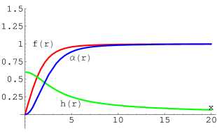
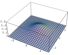
a) Functions $f(r)$, $h(r)$ and $\alpha(r)$ and b), c) Energy density for $h_{0}=0.6$

       

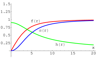
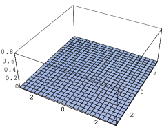
a) Functions $f(r)$, $h(r)$ and $\alpha(r)$ and b), c) Energy density for $h_{0}=0.9$

Figure 1: Field Profiles and Energy Densities for Semi-local Topological Defects

4 One-loop correction to the masses of
semi-local self-dual topological solitons

Casimir energies

The starting point for computing the quantum corrections to the soliton mass is the evaluation of the zero-point oscillations of the fields around both the soliton and the vacuum. The measurement of the zero-point soliton energy with respect to the vacuum energy shows a strong analogy with the Casimir effect, where the plates are substituted by the soliton profile.

Let us first consider small fluctuations around the semi-local soliton by writing:

$$\Phi(\vec{x})=S(\vec{x})+\delta S(x_{0},\vec{x})\hskip 42.67912pt,\hskip 42.67912ptA_{j}(\vec{x})=V_{j}(\vec{x})+\delta a_{j}(x_{0},\vec{x})\qquad.$$

By $S(\vec{x})$ and $V_{k}(\vec{x})$ we respectively denote the scalar and vector fields of the topological soliton solution, whereas $\delta S(x_{0},\vec{x})$ and $\delta a_{j}(x_{0},\vec{x})$ calibrate the small deviations of the bosonic fields with respect to the classical solution. Of course, not all fluctuations are physically relevant, and we should avoid pure gauge deformations. In order to do so, we impose the Weyl/background gauge condition:

$$A_{0}(x_{0},\vec{x})=0\qquad\qquad,\qquad\qquad\partial_{j}\delta a_{j}(x_{0},\vec{x})+\frac{i}{2}(S^{\dagger}(\vec{x})\delta S(x_{0},\vec{x})-\delta S^{\dagger}(x_{0},\vec{x})S(\vec{x}))=0\qquad.$$

Under these constraints, the ground state energy in the topological sectors up to ${\cal O}(\delta^{3})$ order (one-loop) is:

$$H^{(2)}={v^{2}\over 2}\int\,d^{2}x\left\{\frac{\partial\delta\xi^{T}}{\partial x_{0}}\frac{\partial\delta\xi}{\partial x_{0}}+\delta\xi^{T}K\delta\xi+\delta\chi^{*}K^{G}\delta\chi\right\}\qquad,$$ (11)

where the bosonic fluctuations are arranged in the column vector

$$\delta\xi(x_{0},\vec{x})=\left(\begin{array}[]{c}\delta a_{1}(x_{0},\vec{x})\\ \delta a_{2}(x_{0},\vec{x})\\ \delta S_{1}^{1}(x_{0},\vec{x})\\ \delta S_{1}^{2}(x_{0},\vec{x})\\ \delta S_{2}^{1}(x_{0},\vec{x})\\ \delta S_{2}^{2}(x_{0},\vec{x})\end{array}\right)\qquad\qquad,$$

and $\delta\chi(\vec{x})$ corresponds to ghost fluctuations. $K$ and $K^{G}$ are second-order differential operators. $K$ is matrix-valued and fairly complicated

$$K=\left(\begin{array}[]{cccccc}A&0&-2\nabla_{1}S_{1}^{2}&2\nabla_{1}S_{1}^{1}&-2\nabla_{1}S_{2}^{2}&2\nabla_{1}S_{2}^{1}\\ 0&A&-2\nabla_{2}S_{1}^{2}&2\nabla_{2}S_{1}^{1}&-2\nabla_{2}S_{2}^{2}&2\nabla_{2}S_{2}^{1}\\ -2\nabla_{1}S_{1}^{2}&-2\nabla_{2}S_{1}^{2}&B&-2V_{k}\partial_{k}&S_{1}^{1}S_{2}^{1}+S_{1}^{2}S_{2}^{2}&S_{1}^{1}S_{2}^{2}-S_{1}^{2}S_{2}^{1}\\ 2\nabla_{1}S_{1}^{1}&2\nabla_{2}S_{1}^{1}&2V_{k}\partial_{k}&B&-S_{1}^{1}S_{2}^{2}+S_{1}^{2}S_{2}^{1}&S_{1}^{1}S_{2}^{1}+S_{1}^{2}S_{2}^{2}\\ -2\nabla_{1}S_{2}^{2}&-2\nabla_{2}S_{2}^{2}&S_{1}^{1}S_{2}^{1}+S_{1}^{2}S_{2}^{2}&-S_{1}^{1}S_{2}^{2}+S_{1}^{2}S_{2}^{1}&C&-2V_{k}\partial_{k}\\ 2\nabla_{1}S_{2}^{1}&2\nabla_{2}S_{2}^{1}&S_{1}^{1}S_{2}^{2}-S_{1}^{2}S_{2}^{1}&S_{1}^{1}S_{2}^{1}+S_{1}^{2}S_{2}^{2}&2V_{k}\partial_{k}&C\end{array}\right)\qquad,$$

and $K^{G}$ is the scalar differential operator:

$$K^{G}=-\partial_{k}\partial_{k}+|S_{1}|^{2}+|S_{2}|^{2}\quad.$$

In all these formulas, the notation is

$$S(\vec{x})=\left(\begin{array}[]{c}S_{1}(\vec{x})\\ S_{2}(\vec{x})\end{array}\right)=\left(\begin{array}[]{c}S_{1}^{1}(\vec{x})+iS_{1}^{2}(\vec{x}\\ S_{2}^{1}(\vec{x})+iS_{2}^{2}(\vec{x})\end{array}\right)\qquad\qquad,$$

and analogously for $\delta S$. The covariant derivatives are $\nabla_{j}S_{M}^{a}=\partial_{j}S_{M}^{a}+\varepsilon^{ab}V_{j}S_{M}^{b}$, and the differential operators in the diagonal of $K$ take the form

$$A = -\partial_{k}\partial_{k}+|S_{1}|^{2}+|S_{2}|^{2}\qquad,\qquad B=-\partial_{k}\partial_{k}+\frac{1}{2}(3|S_{1}|^{2}+|S_{2}|^{2}+2V_{k}V_{k}-1)\quad,$$

$$C = -\partial_{k}\partial_{k}+\frac{1}{2}(|S_{1}|^{2}+3|S_{2}|^{2}+2V_{k}V_{k}-1)\,\,.$$

The energy due to the zero point fluctuations around the vacuum must be subtracted. As is fairly obvious, the Hamiltonian for the vacuum fluctuations has exactly the same form as (11) for the vacuum values: $S_{1}=1,S_{2}=0,V_{1}=V_{2}=0$. We shall denote by $K_{0}$ and $K^{G}_{0}$ the operators $K$ and $K^{G}$ in the vacuum background.

When all the fluctuation modes are unoccupied, we formally obtain the contribution to the semi-local topological soliton ground state energy as a difference between two “super-traces” of differential operators acting on column vectors of $L^{2}({\mathbb{R}}^{2})$ functions. The first super-trace comes from (the star stresses the fact that zero modes do not contribute to the trace) oscillations of the fields around the soliton,

$$\bigtriangleup E_{\rm TS}=\frac{\hbar m}{2}\cdot\left({\rm Tr}^{*}K^{{1\over 2}}-{\rm Tr}^{*}\left(K^{G}\right)^{{1\over 2}}\right)=\frac{\hbar m}{2}\cdot{\rm STr}^{*}K^{{1\over 2}}\qquad,$$

and the second one accounts for vacuum fluctuations of the fields:

$$\bigtriangleup E_{0}=\frac{\hbar m}{2}\cdot\left({\rm Tr}K_{0}^{{1\over 2}}-{\rm Tr}\left(K_{0}^{G}\right)^{{1\over 2}}\right)={\rm STr}K_{0}^{{1\over 2}}\qquad.$$

Therefore,

$$\bigtriangleup M_{\rm TS}^{C}=\bigtriangleup E_{\rm TS}-\bigtriangleup E_{0}={\hbar m\over 2}\left({\rm STr^{*}}\,K^{{1\over 2}}-{\rm STr}\,K_{0}^{{1\over 2}}\right)$$ (12)

formally measures the semi-local topological soliton Casimir energy.

Before proceeding, a further explanation of how we choose small fluctuations belonging to $L^{2}({\mathbb{R}}^{2})$ deserves a pause. Following the conventional QFT approach, we put the system in a very large but finite two-dimensional box and impose periodic boundary conditions on $\delta\xi(x_{0},\vec{x})$ and $\delta\chi(\vec{x})$. In Appendices II, III, and IV of Reference [22] it is shown that taking the infinite area limit at the end leaves no remnants for kinks and self-dual vortices. Thus, this procedure uses invisible boundary conditions in such a way that, at intermediate stages, one works on circles or genus one Riemann Surfaces. Nevertheless, the rapid (exponential) decay of the Higgs field to its vacuum value in these cases ensures that, starting from large lengths or areas, there will be a very small dependence of the results on the size. Except for the embedded ANO vortices, all the Higgs fields of the semi-local self-dual topological solitons decay to their vacuum values as ${1\over r^{k}}$ for some positive $k$. Therefore, we expect a more significant dependence on the size of the box for these less concentrated solitons.

We might try topological boundary conditions like those used in Reference [14] for the bosonic and supersymmetric kink. In this planar gauge theoretical setting, the analogous form of the anti-periodic boundary conditions would be:

$$\delta\Phi(x_{1},x_{2})=e^{i\int_{P_{0}}^{P_{mL}}\,[V_{k}(\vec{x}^{\prime})dx_{k}^{\prime}\,]}\cdot\delta\Phi(x_{1}+mL,x_{2}+mL)\qquad.$$

The line integral is along a path starting at the point $P_{0}=(x_{1},x_{2})$, ending at $P_{mL}=(x_{1}+mL,x_{2}+mL)$, and passing through regions far away from the vortex core. These twisted boundary conditions are also invisible in the sense that no boundary is introduced. Rather, the fact that we are dealing with a non-trivial line bundle of first Chern class equal to one over a genus one Riemann surface is taken into account. In a purely bosonic framework, however, the twisted boundary conditions, like periodic boundary conditions, will not leave any mark at the infinite area limit.

Counter-term energies

The Casimir energy of the previous Section is of order $\hbar$, and this is also the order of the counter-terms found in Section 2. Thus, the one-loop semi-local topological soliton mass also receives contributions from the counter-terms for scalar and vector fields. At the self-dual limit $\kappa^{2}=1$, these contributions are

$$\Delta M_{c.t.}^{S}=\frac{\hbar\,m}{2}[4I(1)+I(0)]\,\int\,d^{2}x\,(1-|S_{1}|^{2}-|S_{2}|^{2})\,\,\,,\,\,\,\Delta M_{c.t.}^{A}=-\hbar\,m\,[I(1)+I(0)]\int\,d^{2}x\,V_{k}V_{k}\quad.$$

We now reshuffle the sum of these two quantities into two pieces, respectively proportional to $I(1)$ and $I(0)$:

$$\bigtriangleup M_{\rm c.t.}^{\rm I(1)}=\frac{\hbar\,m}{2}\,I(1)\,\Sigma^{(1)}(S,V_{k})\qquad,\qquad\bigtriangleup M_{\rm c.t.}^{\rm I(0)}=\frac{\hbar\,m}{2}\,I(0)\,\Sigma^{(0)}(S,V_{k})\qquad,$$ (13)

where

$$\Sigma^{(1)}(S,V_{k})=4\int\,d^{2}x\,(1-|S_{1}|^{2}-|S_{2}|^{2}-{1\over 2}V_{k}V_{k})\,\,,\,\,\Sigma^{(0)}(S,V_{k})=\int\,d^{2}x\,\left(1-|S_{1}|^{2}-|S_{2}|^{2}-2V_{k}V_{k}\right)\,.$$

The total contribution to the one-loop mass shifts from the mass renormalization counter-terms is:

$$\bigtriangleup M_{\rm c.t.}=\bigtriangleup M_{\rm c.t.}^{\rm I(1)}+\bigtriangleup M_{\rm c.t.}^{\rm I(0)}\qquad.$$

Deformation of the first-order equations

It follows from the classical degeneracy of vortices that there are some static deformations of a topological solution that do not cost energy at the tree level: those that give rise to a new self-dual soliton. Therefore, the dimension of the kernel of the operator $K$ ruling the bosonic small fluctuations around the topological soliton should be equal to the dimension of the moduli space of self-dual semi-local soliton solutions. To check this, we proceed as in the previous Section by expanding the bosonic fields around the solution, but this time we consider only static small fluctuations:

$$\Phi(\vec{x})=S(\vec{x})+\delta S(\vec{x})\hskip 42.67912pt,\hskip 42.67912ptA_{j}(\vec{x})=V_{j}(\vec{x})+\delta a_{j}(\vec{x})\qquad.$$

The modified fields are still solutions of the first-order equations if (14) and (15) are satisfied:

$$F_{12}={1\over 2}(1-\Phi^{\dagger}\Phi)\Leftrightarrow-\partial_{2}\delta a_{1}+\partial_{1}\delta a_{2}+\frac{1}{2}(S^{\dagger}\delta S+\delta S^{\dagger}S)=0\qquad,$$ (14)

and

$$D_{1}\Phi+iD_{2}\Phi=0\Leftrightarrow(\nabla_{1}+i\nabla_{2})\delta S-i(\delta a_{1}+i\delta a_{2})S=0\qquad,$$ (15)

where $\nabla_{k}=\partial_{k}-iV_{k}$. Also as in the previous Section, in order to avoid pure gauge fluctuations we set the static background gauge:

$$\partial_{j}\delta a_{j}(\vec{x})+\frac{i}{2}(S^{\dagger}\delta S-\delta S^{\dagger}S)=0\quad.$$

Thus, the tangent space to the moduli space of self-dual vortices is the kernel of the first-order deformation operator ${\cal D}$:

$${\cal D}=\left(\begin{array}[]{cccccc}-\partial_{2}&\partial_{1}&S_{1}^{1}&S_{1}^{2}&S_{2}^{1}&S_{2}^{2}\\ -\partial_{1}&-\partial_{2}&-S_{1}^{2}&S_{1}^{1}&-S_{2}^{2}&S_{2}^{1}\\ S_{1}^{1}&-S_{1}^{2}&-\partial_{2}+V_{1}&-\partial_{1}-V_{2}&0&0\\ S_{1}^{2}&S_{1}^{1}&\partial_{1}+V_{2}&-\partial_{2}+V_{1}&0&0\\ S_{2}^{1}&-S_{2}^{2}&0&0&-\partial_{2}+V_{1}&-\partial_{1}-V_{2}\\ S_{2}^{2}&S_{2}^{1}&0&0&\partial_{1}+V_{2}&-\partial_{2}+V_{1}\\ \end{array}\right)\qquad.$$

One easily checks that $K={\cal D}^{\dagger}{\cal D}$, and it is also possible to prove that the Kernel of ${\cal D}^{\dagger}$ is empty [24]. Thus, $K$ and ${\cal D}$ have the same kernel and the dimension of that kernel is the dimension of the classical moduli space: $4l$.

Zeta-function regularization

The zero-point energies for the topological soliton and the vacuum are formally super-traces: the differences of traces of differential operators. Such traces are divergent quantities. The standard procedure for dealing with this delicate point is understanding these traces as the generalized zeta functions of the corresponding differential operators; see [12]-[6]-[9]. Given a differential operator $A$ acting on an $L^{2}$ space of functions, the corresponding generalized zeta function is:

$$\zeta_{A}(s)=\sum_{{\rm Spec}\,A}\,\lambda_{n}^{-s}\qquad\qquad,\qquad\qquad s\in{\mathbb{C}}\qquad,$$

where $\lambda_{n}$ are the eigenvalues of $A$. We shall regularize the zero-point energies in the form:

$$\Delta E_{TS}(s)=\frac{\hbar\mu}{2}\left({\mu^{2}\over m^{2}}\right)^{s}\left\{\zeta_{K}(s)-\zeta_{K^{G}}(s)\right\}\hskip 17.07182pt,\hskip 17.07182pt\Delta E_{0}(s)=\frac{\hbar\mu}{2}\left({\mu^{2}\over m^{2}}\right)^{s}\left\{\zeta_{K_{0}}(s)-\zeta_{K^{G}_{0}}(s)\right\}\quad,$$

i.e., by assigning to the meromorphic generalized zeta functions the value obtained by analytic continuation at the point $s$ of the $s$ -complex plane. The physical limit is:

$$\Delta M_{TS}^{C}=\lim_{s\rightarrow-\frac{1}{2}}\Delta M_{TS}^{C}(s)=\lim_{s\rightarrow-\frac{1}{2}}\left(\Delta E_{TS}(s)-\Delta E_{0}(s)\right).$$

Because $K_{0}$ and $K^{G}_{0}$ are free Schrödinger operators, their zeta functions are well known [11, 15]:

$$\zeta_{K_{0}}(s)=\frac{m^{2}L^{2}}{\pi}\cdot\frac{\Gamma[s-1]}{\Gamma(s)}+\frac{m^{2}L^{2}}{2\pi}\cdot\frac{1}{(s-1)\Gamma(s)}\hskip 28.45274pt,\hskip 28.45274pt\zeta_{K^{G}_{0}}(s)=\frac{m^{2}L^{2}}{4\pi}\cdot\frac{\Gamma[s-1]}{\Gamma(s)}\quad,$$

where $\Gamma(s)$ and $\gamma[s,a]$ are the complete and incomplete Euler Gamma functions, respectively.

The contribution from the mass counter-terms also involves divergent quantities proportional to the integrals $I(1)$ and $I(0)$. To regularize these integrals, we apply the residue theorem to integrate $I(c)$ in the complex $k_{0}$-plane. On a square of area $m^{2}L^{2}$ each integral becomes a infinite sum over discrete momenta:

$$I(c)={1\over 2}\int{d^{2}k\over(2\pi)^{2}}{1\over\sqrt{\vec{k}\cdot\vec{k}+c}}={1\over 2}{1\over m^{2}L^{2}}\sum_{\vec{k}\in{\mathbb{Z}}^{2}}\frac{1}{\sqrt{\vec{k}\cdot\vec{k}+c}}\qquad.$$

Accordingly, these integrals are the generalized zeta functions of the Euclidean Klein-Gordon and Laplacian operators evaluated at $s={1\over 2}$. In this way, we also define the mass renormalization correction as a meromorphic function in the complex $s$-plane:

$$\Delta M_{TS}^{R}(s)={\hbar\over 2\mu L^{2}}\left({\mu^{2}\over m^{2}}\right)^{s}\left(\zeta_{-\bigtriangleup+1}(s)\Sigma^{(1)}(S,V_{k})+\zeta_{-\bigtriangleup}(s)\Sigma^{(0)}(S,V_{k})\right)\qquad,$$

and take the physical limit:

$$\Delta M_{TS}^{R}=\lim_{s\rightarrow{1\over 2}}\Delta M_{TS}^{R}(s)\qquad\qquad.$$

While $-\bigtriangleup+1$ is exactly $K^{G}_{0}$, and its zeta function has been written above, calculation of $\zeta_{\bigtriangleup}(s)$ is a bit tricky. From the partition function for the Laplacian, via the Mellin transform, we have:

$$\zeta_{-\bigtriangleup}(s)={m^{2}L^{2}\over 4\pi}\lim_{\varepsilon\rightarrow 0}{1\over\Gamma(s)}\left(\int_{0}^{1}\,d\beta\,\beta^{s-2}\,e^{-\varepsilon\beta}+\int_{1}^{\infty}\,d\beta\,\beta^{s-2}\,e^{-\varepsilon\beta}\right)\qquad,$$

or,

$$\zeta_{-\bigtriangleup}(s)={m^{2}L^{2}\over 4\pi}\lim_{\varepsilon\rightarrow 0}{1\over\varepsilon^{s-1}\Gamma(s)}\left(\gamma[s-1,\varepsilon]+\Gamma[s-1,\varepsilon]\right)\qquad.$$

Because $\gamma[s-1,\varepsilon]{\footnotesize{\begin{array}[]{c}\\ \cong\\ \varepsilon\rightarrow 0\end{array}}}{\Large{\frac{\varepsilon^{s-1}}{s-1}-{\varepsilon^{s}\over s}}}$ and $\Gamma[s-1,\varepsilon]{\footnotesize{\begin{array}[]{c}\\ \cong\\ \varepsilon\rightarrow 0\end{array}}}{\large{\Gamma[s-1]}}$ , we obtain:

$$\zeta_{-\bigtriangleup}(s)={m^{2}L^{2}\over 4\pi}\cdot{1\over(s-1)\Gamma(s)}\qquad{\rm if}\quad{\rm Re}\,\,{\rm s}<1\qquad\qquad.$$

We finally find:

$$I(1)={1\over 2m^{2}L^{2}}\zeta_{-\bigtriangleup+1}({1\over 2})={1\over 8\pi}{\Gamma(-{1\over 2})\over\Gamma({1\over 2})}=-{1\over 4\pi}\qquad,\qquad I(0)={1\over 2m^{2}L^{2}}\zeta_{-\bigtriangleup}({1\over 2})=-\frac{1}{4\pi\sqrt{\pi}}\qquad.$$

Contrary to the kink cases, which are one-dimensional problems, a finite answer is obtained in the regularized integrals via the associated zeta functions. The reason is that in this two-dimensional problem the physical limit $s={1\over 2}$ is not a pole of the zeta functions and only finite renormalizations will be necessary.

5 The semi-local topological soliton heat kernel
and generalized zeta function

Control of $\zeta_{K}(s)$ and $\zeta_{K^{G}}(s)$ is much more difficult. A convenient way for dealing with the zeta functions of differential operators acting on infinite dimensional spaces is by means of heat kernel techniques. In this Section, we shall develop this method, applied to our soliton operators.

The heat kernel of a differential operator. Seeley densities

The heat equation kernel of a $N\times N$ matrix differential operator of the general form

$${\cal K}={\cal K}_{0}+Q_{k}(\vec{x})\partial_{k}+V(\vec{x})$$

is the solution of the ${\cal K}$-heat equation

$$\left(\frac{\partial}{\partial\beta}{\mathbb{I}}+{\cal K}\right)K_{{\cal K}}(\vec{x},\vec{y};\beta)=0$$

with initial condition: $K_{{\cal K}}(\vec{x},\vec{y};0)={\mathbb{I}}\cdot\delta^{(2)}(\vec{x}-\vec{y})$. We are particularly interested in the diagonal $\vec{x}=\vec{y}$ heat-kernel, because the Mellin transform of the partition function

$${\rm Tr}\,e^{-\beta{\cal K}}={\rm tr}\int_{{\mathbb{R}}^{2}}\,d^{2}\vec{x}\,K_{{\cal K}}(\vec{x},\vec{x};\beta)$$

gives the generalized zeta function.

To find the kernel, one writes [8]

$$K_{{\cal K}}(\vec{x},\vec{y};\beta)=C_{\cal K}(\vec{x},\vec{y};\beta)K_{{\cal K}_{0}}(\vec{x},\vec{y};\beta)\qquad,$$

where ${\cal K}_{0}$ is the operator ${\cal K}$ very distant from the origin, where $Q_{k}(\vec{x})$ and $V(\vec{x})$ take their asymptotic constant vacuum values. $C_{\cal K}(\vec{x},\vec{y};\beta)$ satisfies the $N\times N$-matrix transfer equation

$$\left\{{\partial\over\partial\beta}{\mathbb{I}}+{x_{k}-y_{k}\over\beta}(\partial_{k}{\mathbb{I}}-{1\over 2}Q_{k})-\bigtriangleup{\mathbb{I}}+Q_{k}\partial_{k}+V\rule[-7.22743pt]{0.0pt}{14.45377pt}\right\}C_{\cal K}(\vec{x},\vec{y};\beta)=0$$

and is the unit matrix $C_{\cal K}(\vec{x},\vec{y};0)={\mathbb{I}}$ at infinite temperature.

Solving the transfer equation as an inverse-temperature power series expansion,

$$C_{\cal K}(\vec{x},\vec{y};\beta)=\sum_{n=0}^{\infty}c_{n}(\vec{x},\vec{y};{\cal K})\beta^{n},$$

the PDE equation becomes tantamount to the recurrence relation between the densities $c_{n}(\vec{x},\vec{y};{\cal K})$:

$$[n{\mathbb{I}}+(x_{k}-y_{k})(\partial_{k}{\mathbb{I}}-{1\over 2}Q_{k})]c_{n}(\vec{x},\vec{y};{\cal K})=[\bigtriangleup{\mathbb{I}}-Q_{k}\partial_{k}-V]c_{n-1}(\vec{x},\vec{y};{\cal K})\hskip 28.45274pt,\hskip 28.45274ptn\geq 1$$

to be started from: $c_{0}(\vec{x},\vec{y};{\cal K})={\mathbb{I}}$. While it is easy to find the first diagonal density, $c_{1}(\vec{x},\vec{x};{\cal K})=-V(\vec{x})$, the determination of higher-order densities becomes more and more involved. To make the problem more tractable, we introduce the following notation:

$${}^{(\alpha_{1},\alpha_{2})}C_{n}^{AB}(\vec{x})=\lim_{\vec{y}\rightarrow\vec{x}}\frac{\partial^{\alpha_{1}+\alpha_{2}}[c_{n}]_{AB}(\vec{x},\vec{y};{\cal K})}{\partial x_{1}^{\alpha_{1}}\partial x_{2}^{\alpha_{2}}}\hskip 28.45274pt,\hskip 28.45274pt[{c}_{n}]_{AB}(\vec{x},\vec{x};{\cal K})={}^{(0,0)}C_{n}^{AB}(\vec{x})\qquad.$$

Thus, at the $\vec{y}\rightarrow\vec{x}$ limit the recurrence relations between densities and partial derivatives of densities can be written in compact form:

$$(k+\alpha_{1}+\alpha_{2}+1){}^{(\alpha_{1},\alpha_{2})}C_{k+1}^{AB}(\vec{x})={}^{(\alpha_{1}+2,\alpha_{2})}C_{k}^{AB}(\vec{x})+{}^{(\alpha_{1},\alpha_{2}+2)}C_{k}^{AB}(\vec{x})-$$

$$-\sum_{d=1}^{N}\sum_{r=0}^{\alpha_{1}}\sum_{t=0}^{\alpha_{2}}{\alpha_{1}\choose r}{\alpha_{2}\choose t}\left[\frac{\partial^{r+t}Q^{AD}_{1}}{\partial x_{1}^{r}\partial x_{2}^{t}}{}^{(\alpha_{1}-r+1,\alpha_{2}-t)}C_{k}^{DB}(\vec{x})\right.+$$

$$+\left.\frac{\partial^{r+t}Q^{AD}_{2}}{\partial x_{1}^{r}\partial x_{2}^{t}}{}^{(\alpha_{1}-r,\alpha_{2}-t+1)}C_{k}^{DB}(\vec{x})\right]+$$

$$+\frac{1}{2}\sum_{d=1}^{N}\sum_{r=0}^{\alpha_{1}-1}\sum_{t=0}^{\alpha_{2}}\alpha_{1}{\alpha_{1}-1\choose r}{\alpha_{2}\choose t}\frac{\partial^{r+t}Q^{AD}_{1}}{\partial x_{1}^{r}\partial x_{2}^{t}}{}^{(\alpha_{1}-1-r,\alpha_{2}-t)}C_{k+1}^{DB}(\vec{x})+$$

$$+\frac{1}{2}\sum_{d=1}^{N}\sum_{r=0}^{\alpha_{2}-1}\sum_{t=0}^{\alpha_{1}}\alpha_{2}{\alpha_{2}-1\choose r}{\alpha_{1}\choose t}\frac{\partial^{r+t}Q^{AD}_{2}}{\partial x_{1}^{t}\partial x_{2}^{r}}{}^{(\alpha_{1}-t,\alpha_{2}-1-r)}C_{k+1}^{DB}(\vec{x})-$$

$$-\sum_{d=1}^{N}\sum_{r=0}^{\alpha_{2}}\sum_{t=0}^{\alpha_{1}}{\alpha_{1}\choose t}{\alpha_{2}\choose r}\frac{\partial^{r+t}V^{AD}}{\partial x_{1}^{t}\partial x_{2}^{r}}{}^{(\alpha_{1}-t,\alpha_{2}-r)}C_{k}^{DB}(\vec{x})$$

to be solved starting from

$$c_{0}(\vec{x},\vec{x};{\cal K})={\mathbb{I}}\Rightarrow\left\{\begin{array}[]{c}{}^{(\alpha,\beta)}C_{0}^{AB}(\vec{x})=0,\,{\rm if}\,\alpha\neq 0,{{\rm and}/{\rm or}}\,\beta\neq 0\\ {}^{(0,0)}C_{0}^{AA}(\vec{x})=1,\,A=1,2,\cdots,N\end{array}\right.\qquad.$$

The Mellin transform of the asymptotic expansion

We must now deal with the cases $N=6$ and $N=1$, respectively for the operators $K$ and $K^{G}$. A good approximation to the generalized zeta functions of both operators is obtained from the Mellin transform [9]

$$\zeta_{K}(s)={1\over\Gamma(s)}\int_{0}^{\infty}\,d\beta\,\beta^{s-1}\,{\rm Tr}\,e^{-\beta K}\qquad,\qquad\zeta_{K^{G}}(s)={1\over\Gamma(s)}\int_{0}^{\infty}\,d\beta\,\beta^{s-1}\,{\rm Tr}\,e^{-\beta K^{G}}$$

applied to the high-temperature expansion of the partition functions

$${\rm Tr}e^{-\beta K} = {1\over 4\pi\beta}\sum_{n=0}^{\infty}\beta^{n}\cdot\left(e^{-\beta}\sum_{A=1}^{4}[c_{n}^{I}(K)]_{AA}+\sum_{A=5}^{6}[c^{O}_{n}(K)]_{AA}\right)$$

$${\rm Tr}e^{-\beta K^{\rm G}} = {e^{-\beta}\over 4\pi\beta}\sum_{n=0}^{\infty}\beta^{n}c_{n}(K^{\rm G})\qquad,$$

where

$$[c_{n}^{I}(K)]_{AA} = \int\,d^{2}x\,e^{-\beta}[c_{n}]_{AA}(\vec{x},\vec{x};K)\quad,\quad A=1,2,3,4$$

$${[c_{n}^{O}(K)]}_{AA} = \int\,d^{2}x\,[c_{n}]_{AA}(\vec{x},\vec{x};K)\quad,\quad A=5,6\quad,\quad{[c_{n}(K^{G})]}=\int\,d^{2}x\,[c_{n}](\vec{x},\vec{x};K^{G})\,\,.$$

The factor $e^{-\beta}$, which appears in front of $[c_{n}(K)]_{AA}$ for $A=1,2,3,4$, obeys the fact that the corresponding modes in $\xi$ have one unit of mass, while the modes for $A=5,6$ are massless. The generalized zeta functions are thus divided as sums of meromorphic -high-temperature regime- and entire -to be neglected, low temperature regime- functions of $s$:

$$\zeta_{K}(s) = {1\over 4\pi\Gamma(s)}\sum_{n=0}^{\infty}\left\{\sum_{A=1}^{4}\int_{0}^{1}\,d\beta\,\beta^{s+n-2}[c_{n}^{I}(K)]_{AA}e^{-\beta}+\sum_{A=5}^{6}\int_{0}^{1}\,d\beta\,\beta^{s+n-2}[c_{n}^{O}(K)]_{AA}\right\}$$

$$+ {1\over\Gamma(s)}\int_{1}^{\infty}\,d\beta\,{\rm Tr}^{*}e^{-\beta K}$$

$$= \sum_{n=0}^{\infty}\left\{\sum_{A=1}^{4}[c_{n}^{I}(K)]_{AA}\frac{\gamma[s+n-1,1]}{4\pi\Gamma(s)}+\sum_{A=5}^{6}[c_{n}^{O}(K)]_{AA}\frac{1}{4\pi\Gamma(s)(s+n-1)}\right\}+{1\over\Gamma(s)}B_{K}(s)$$

$$\zeta_{K^{G}}(s) = {1\over\Gamma(s)}\sum_{n=0}^{\infty}\int_{0}^{1}\,d\beta\,\beta^{s+n-2}c_{n}(K^{G})e^{-\beta}+{1\over\Gamma(s)}\int_{1}^{\infty}\,d\beta\,{\rm Tr}^{*}e^{-\beta K^{G}}$$

$$= \sum_{n=0}^{\infty}c_{n}(K^{G})\frac{\gamma[s+n-1,1]}{4\pi\Gamma(s)}+{1\over\Gamma(s)}B_{K^{G}}(s)\qquad,$$

where $\gamma[s+n-1,1]$ are incomplete Euler Gamma functions. We shall neglect the entire parts $B(K)$ and $B(K^{G})$ and keep a finite number of terms, $N_{0}$, in future use of these generalized zeta functions for the regularization of ultraviolet divergences.

The high-temperature one-loop semi-local vortex mass shift formula

The contribution of the $c_{1}$ coefficients to the semi-local topological soliton Casimir energy is

$$\Delta M_{TS}^{(1)C}(s)={\hbar\over 2}\mu\left({\mu^{2}\over m^{2}}\right)^{s}\left\{\left[\sum_{A=1}^{4}[c_{1}^{I}(K)]_{AA}-c_{1}(K^{\rm G})\right]\cdot{\gamma[s,1]\over 4\pi\Gamma(s)}+\sum_{A=5}^{6}[c_{1}^{O}(K)]_{AA}\frac{1}{4\pi s\Gamma(s)}\right\}\qquad,$$

but the first Seeley coefficients due to bosonic and ghost fluctuations, respectively, give:

$$\sum_{A=1}^{4}[c_{1}^{I}(K)]_{AA} = \int\,d^{2}x\,[5-5|S_{1}|^{2}-3|S_{2}|^{2}-2V_{k}V_{k}]$$

$$\sum_{A=5}^{6}[c_{1}^{O}(K)]_{AA} = \int\,d^{2}x\,[1-|S_{1}|^{2}-3|S_{2}|^{2}-2V_{k}V_{k}]$$

$$c_{1}(K^{\rm G}) = \int\,d^{2}x\,[1-|S_{1}|^{2}-|S_{2}|^{2}]\qquad.$$

Therefore,

$$\Delta M_{TS}^{(1)C}(-1/2) = -{\hbar m\over 16\pi}\left\{\left(\Sigma^{(1)}(S,V_{k})+2\int\,d^{2}x\,\left|S_{2}\right|^{2}\right)\cdot{\gamma[-1/2,1]\over\Gamma(1/2)}\right.$$

$$- \left.\left(\Sigma^{(0)}(S,V_{k})-2\int\,d^{2}x\,\left|S_{2}\right|^{2}\right)\cdot\frac{2}{\Gamma(1/2)}\right\}\qquad.$$

On the other hand, the contribution to the one-loop semi-local string tension shift of the mass renormalization counter-terms is:

$$\Delta M_{TS}^{R}(1/2)={\hbar m\over 16\pi}\cdot\left\{\Sigma^{(1)}(S,V_{k})\cdot{\gamma[-1/2,1]\over\Gamma(1/2)}-{2\over\Gamma(1/2)}\cdot\Sigma^{(0)}(S,V_{k})\right\}\qquad,$$

which almost cancels the contribution to the semi-local string Casimir energy density of the $c_{1}$ coefficients. We finally obtain the high-temperature one-loop semi-local topological soliton mass shift formula:

$$\Delta M_{TS} = -{\hbar m\over 16\pi\sqrt{\pi}}\left[\sum_{n=2}^{N_{0}}\,\left\{[\sum_{A=1}^{4}[c_{n}(K)]_{AA}-c_{n}(K^{\rm G})]\cdot\gamma[n-\frac{3}{2},1]+\sum_{A=5}^{6}\frac{[c_{n}(K)]_{AA}}{n-\frac{3}{2}}\right\}+4l\cdot 8\pi\right]$$ (16)

$$- \frac{\hbar m}{8\pi\sqrt{\pi}}\cdot\int\,d^{2}x\,\left|S_{2}\right|^{2}(x_{1},x_{2})\cdot\left(\gamma[-{1\over 2},1]-2\right)\quad.$$

In this final formula (16) there are four types of terms:

• First, polynomial expressions in incomplete Gamma functions times the heat-kernel expansion coefficients for K - saving only the four first diagonal contributions due to massive bosonic particles- and $K^{G}$ -coming from fermionic massive particles. All of them start from the second-order coefficients.

• Second, polynomial expressions in ${1\over n-{3\over 2}}$, including the last two diagonal heat kernel coefficients that collect the contribution of massless Goldstone particles. The starting coefficients are also of second order.

• Third, a factor proportional to $4l$, taking into account the subtraction of the $4l$ zero modes.

• An extra piece proportional to the norm of the second Higgs field due to the imperfect cancelation of the contribution of first-order Seeley coefficients by mass renormalization counter-terms.

Finally, let us mention that by cutting the expansion at a finite number, $N_{0}$, we admit an error - besides the rejected entire parts - which is a priori proportional to $\gamma[N_{0}-{1\over 2},1]\simeq{1\over N_{0}-{1\over 2}}$, for $N_{0}$ large. Nevertheless, as we shall see in the next Section, once all the calculations have been done the degree of convergence of the results is very good, meaning that the proportionality coefficient in that error is very small. The reliability of the method is therefore quite high.

6 Mathematica calculations

Seeley densities for spherically symmetric semi-local vortices

We shall apply (16) to spherically symmetric vortices. The heat kernel local coefficients, however, depend on successive derivatives of the solution. This dependence can increase the error in the estimation of these local coefficients because we are handling an interpolating polynomial as the numerically generated solution, and the successive derivation with respect to $r$ of such a polynomial introduces inaccuracies. Indeed, this operation is plugged into the algorithm that generates the local coefficients in order to speed up this process. It is thus of crucial importance to use the first-order differential equations (4)-(5)-(6) in order to eliminate the derivatives of the solution and to write the local coefficients as expressions that depend only on the fields. Recalling the form of the spherically symmetric solutions,

$$S_{1}^{1}(x_{1},x_{2}) = f(r)\cos\theta\hskip 56.9055ptS_{1}^{2}(x_{1},x_{2})=f(r)\sin\theta$$

$$S_{2}^{1}(x_{1},x_{2}) = h(r)\hskip 82.51282ptS_{2}^{2}(x_{1},x_{2})=0$$

$$V_{1}(x_{1},x_{2}) = -\frac{\alpha(r)}{r}\sin\theta\hskip 48.36958ptV_{2}(x_{1},x_{2})=\frac{\alpha(r)}{r}\cos\theta\qquad,$$

use of the first-order equations shows that:

$$\frac{\partial S_{1}^{1}}{\partial x_{1}} = \frac{f(r)}{r}\left[1-\alpha(r)\cos^{2}\theta\right]\hskip 28.45274pt\frac{\partial S_{1}^{2}}{\partial x_{2}}=\frac{f(r)}{r}\left[1-\alpha(r)\sin^{2}\theta\right]\hskip 28.45274pt\frac{\partial S_{2}^{1}}{\partial x_{2}}=-\frac{h(r)}{r}\alpha(r)\cos\theta$$

$$\frac{\partial S_{1}^{1}}{\partial x_{2}} = -\frac{f(r)}{r}\alpha(r)\cos\theta\sin\theta\hskip 34.14322pt\frac{\partial S_{1}^{2}}{\partial x_{1}}=-\frac{f(r)}{r}\alpha(r))\sin\theta\cos\theta\hskip 28.45274pt\frac{\partial S_{2}^{1}}{\partial x_{1}}=-\frac{h(r)}{r}\alpha(r))\sin\theta$$

$$\frac{\partial V_{1}}{\partial x_{1}} = {\cos 2\theta\over 2}\left[\frac{2f(r)\alpha(r)}{r}+{f^{2}(r)+h^{2}(r)-1\over 2}\right]\hskip 11.38092pt\quad\frac{\partial V_{1}}{\partial x_{2}}=-\cos 2\theta\frac{\alpha(r)}{r^{2}}+{\sin^{2}\theta\over 2}(f^{2}(r)+h^{2}(r)-1)$$

$$\frac{\partial V_{2}}{\partial x_{1}} = -\cos 2\theta\frac{\alpha(r)}{r^{2}}-{\cos^{2}\theta\over 2}(f^{2}(r)+h^{2}(r)-1)\hskip 8.5359pt\hskip 14.22636pt\frac{\partial V_{2}}{\partial x_{2}}=-{\cos 2\theta\over 2}\left[\frac{2f(r)\alpha(r)}{r}+{f^{2}(r)+h^{2}(r)-1\over 2}\right]\qquad.$$

Bearing this in mind, we solve the recurrence relations to find:

$${\rm tr}\,c_{1}^{I}(r) = 5-\frac{2\,{\alpha(r)}^{2}}{r^{2}}-5\,{f(r)}^{2}-3\,{h(r)}^{2}$$

$${\rm tr}\,c_{2}^{I}(r) = \frac{1}{12\,r^{4}}\left[4\,{\alpha(r)}^{4}+27\,r^{4}\,{f(r)}^{4}-8\,r^{2}\,\alpha(r)\,\left(-1+14\,{f(r)}^{2}+{h(r)}^{2}\right)+\right.$$

$$\hskip 22.76228pt+8\,{\alpha(r)}^{2}\,\left(-2-3\,r^{2}+9\,r^{2}\,{f(r)}^{2}+3\,r^{2}\,{h(r)}^{2}\right)+$$

$$\hskip 22.76228pt+\left.{f(r)}^{2}\,\left(56\,r^{2}-64\,r^{4}+34\,r^{4}\,{h(r)}^{2}\right)+r^{4}\,\left(37-32\,{h(r)}^{2}+7\,{h(r)}^{4}\right)\right]$$

$${\rm tr}\,c_{3}^{I}(r) = \frac{1}{120\,r^{6}}\left\{-4\,{\alpha(r)}^{6}-4\,r^{2}\,{\alpha(r)}^{3}\,\left(14+35\,{f(r)}^{2}-36\,{h(r)}^{2}\right)+\right.$$

$$\hskip 25.6073pt+4\,{\alpha(r)}^{4}\,\left(20+9\,r^{2}+32\,r^{2}\,{f(r)}^{2}+26\,r^{2}\,{h(r)}^{2}\right)-$$

$$\hskip 25.6073pt-2\,r^{2}\,\alpha(r)\,\left[57\,r^{2}\,{f(r)}^{4}+{f(r)}^{2}\,\left(32+331\,r^{2}-75\,r^{2}\,{h(r)}^{2}\right)-4\,\left(-1+{h(r)}^{2}\right)\,\left(-16-9\,r^{2}+r^{2}\,{h(r)}^{2}\right)\right]+$$

$$\hskip 25.6073pt+{\alpha(r)}^{2}\,\left[-256-144\,r^{2}-117\,r^{4}+99\,r^{4}\,{f(r)}^{4}-16\,r^{2}\,{h(r)}^{2}+94\,r^{4}\,{h(r)}^{2}-61\,r^{4}\,{h(r)}^{4}+\right.$$

$$\hskip 65.44142pt+\left.2\,r^{2}\,{f(r)}^{2}\,\left(56+183\,r^{2}+19\,r^{2}\,{h(r)}^{2}\right)\right]+$$

$$\hskip 25.6073pt+r^{4}\,\left[-16+151\,r^{2}-29\,r^{2}\,{f(r)}^{6}+\left(32-135\,r^{2}\right)\,{h(r)}^{2}+\left(-16+23\,r^{2}\right)\,{h(r)}^{4}+r^{2}\,{h(r)}^{6}+\right.$$

$$\hskip 34.14322pt+\left.\left.{f(r)}^{4}\,\left(-20+199\,r^{2}-57\,r^{2}\,{h(r)}^{2}\right)+{f(r)}^{2}\,\left(392-321\,r^{2}+2\,\left(-68+111\,r^{2}\right)\,{h(r)}^{2}-27\,r^{2}\,{h(r)}^{4}\right)\right]\right\}$$

$${\rm tr}\,c_{1}^{O}(r) = 1-\frac{2\,{\alpha(r)}^{2}}{r^{2}}-{f(r)}^{2}-3\,{h(r)}^{2}$$

$${\rm tr}\,c_{2}^{O}(r) = \frac{1}{12\,r^{4}}[4\,{\alpha(r)}^{4}-r^{4}\,{f(r)}^{4}+8\,r^{2}\,\alpha(r)\,\left(1+2\,{f(r)}^{2}-{h(r)}^{2}\right)-$$

$$\hskip 22.76228pt-8\,{\alpha(r)}^{2}\,\left(2+r^{2}+r^{2}\,{f(r)}^{2}-5\,r^{2}\,{h(r)}^{2}\right)+2\,r^{2}\,{f(r)}^{2}\,\left(-4+9\,r^{2}\,{h(r)}^{2}\right)+$$

$$\hskip 22.76228pt+r^{4}\,\left(1-8\,{h(r)}^{2}+19\,{h(r)}^{4}\right)]$$

$${\rm tr}\,c_{3}^{O}(r) = \frac{-1}{120\,r^{6}}\left\{4\,{\alpha(r)}^{6}-4\,r^{2}\,{\alpha(r)}^{3}\,\left(-14+9\,{f(r)}^{2}+84\,{h(r)}^{2}\right)-\right.$$

$$\hskip 22.76228pt-4\,{\alpha(r)}^{4}\,\left(20+3\,r^{2}+2\,r^{2}\,\left({f(r)}^{2}+4\,{h(r)}^{2}\right)\right)+$$

$$\hskip 22.76228pt+{\alpha(r)}^{2}\,\left[256+48\,r^{2}-3\,r^{4}+45\,r^{4}\,{f(r)}^{4}+2\,r^{2}\,\left(-40+89\,r^{2}\right)\,{h(r)}^{2}-115\,r^{4}\,{h(r)}^{4}+\right.$$

$$\hskip 71.13188pt+\left.2\,r^{2}\,{f(r)}^{2}\,\left(8+5\,r^{2}-35\,r^{2}\,{h(r)}^{2}\right)\right]-$$

$$\hskip 22.76228pt-2\,r^{2}\,\alpha(r)\,\left[53\,r^{2}\,{f(r)}^{4}+4\,\left(-1+{h(r)}^{2}\right)\,\left(-16-3\,r^{2}+7\,r^{2}\,{h(r)}^{2}\right)-{f(r)}^{2}\,\left(32+17\,r^{2}+47\,r^{2}\,{h(r)}^{2}\right)\right]+$$

$$\hskip 22.76228pt+r^{4}\,\left[16+3\,r^{2}+3\,r^{2}\,{f(r)}^{6}-\left(32+19\,r^{2}\right)\,{h(r)}^{2}+\left(16+23\,r^{2}\right)\,{h(r)}^{4}+33\,r^{2}\,{h(r)}^{6}+\right.$$

$$\hskip 51.21504pt+\left.\left.{f(r)}^{4}\,\left(52-r^{2}+39\,r^{2}\,{h(r)}^{2}\right)+{f(r)}^{2}\,\left(-24-5\,r^{2}+\left(-72+22\,r^{2}\right)\,{h(r)}^{2}+69\,r^{2}\,{h(r)}^{4}\right)\right]\right\}$$

$$c_{1}^{G}(r) = 1-{f(r)}^{2}-{h(r)}^{2}$$

$$c_{2}^{G}(r) = \frac{1}{6\,r^{2}}\left[3\,r^{2}+2\,r^{2}\,{f(r)}^{4}-\left(5\,r^{2}+4\,{\alpha(r)}^{2}\right)\,{h(r)}^{2}+2\,r^{2}\,{h(r)}^{4}+\right.$$

$$\hskip 22.76228pt\left.+{f(r)}^{2}\,\left(-4-5\,r^{2}+8\,\alpha(r)-4\,{\alpha(r)}^{2}+4\,r^{2}\,{h(r)}^{2}\right)\right]$$

$$c_{3}^{G}(r) = \frac{-1}{60\,r^{4}}\left\{-10\,r^{4}+4\,r^{4}\,{f(r)}^{6}+\left[23\,r^{4}-8\,r^{2}\,\alpha(r)+16\,\left(1+r^{2}\right)\,{\alpha(r)}^{2}+32\,{\alpha(r)}^{3}+16\,{\alpha(r)}^{4}\right]\,{h(r)}^{2}+\right.$$

$$\hskip 25.6073pt+r^{2}\,\left[-17\,r^{2}+8\,\alpha(r)-16\,{\alpha(r)}^{2}\right]\,{h(r)}^{4}+4\,r^{4}\,{h(r)}^{6}+$$

$$\hskip 25.6073pt+r^{2}\,{f(r)}^{4}\,\left[-24-17\,r^{2}+40\,\alpha(r)-16\,{\alpha(r)}^{2}+12\,r^{2}\,{h(r)}^{2}\right]+$$

$$\hskip 25.6073pt+{f(r)}^{2}\,\left[-32\,{\alpha(r)}^{3}+16\,{\alpha(r)}^{4}+8\,r^{2}\,\alpha(r)\,\left(-5+6\,{h(r)}^{2}\right)+16\,{\alpha(r)}^{2}\,\left(1+r^{2}-2\,r^{2}\,{h(r)}^{2}\right)\right.+$$

$$\left.\hskip 25.6073pt+\left.r^{2}\,\left(24+23\,r^{2}-2\,\left(10+17\,r^{2}\right)\,{h(r)}^{2}+12\,r^{2}\,{h(r)}^{4}\right)\right]\right\}\qquad,$$

etcetera, by means of a computing program implemented on a PC with Mathematica.

One-loop mass shift for the mass of the ANO vortex

Denoting simply

$${\rm tr}\,c_{n}^{I}=2\pi\int_{0}^{\infty}\,dr\,r{\rm tr}\,c_{n}^{I}(r)\quad,\quad{\rm tr}\,c_{n}^{O}=2\pi\int_{0}^{\infty}\,dr\,r{\rm tr}\,c_{n}^{O}(r)\quad,\quad c_{n}^{G}=2\pi\int_{0}^{\infty}\,dr\,rc_{n}^{G}(r)\qquad,$$

by plugging the NO vortex solution in these expressions, i.e. the case $h_{0}=0.0$, embedded in this model, we find the Table at the left:

	$h_{0}=0.0$
$n$	${\rm tr}\,c_{n}^{I}$	${\rm tr}\,c_{n}^{O}$	$c_{n}^{G}$
1	-41.4469	-91.8429	12.599
2	30.3736	0.96286	2.61518
3	12.9447	-0.0592415	0.32005
4	4.22603	0.001512548	0.0230445
5	1.05059	0.000758663	0.0013023
6	0.20900	-0.00023912	0.0000698185

$N_{0}$	$\Delta M_{V}(N_{0})$
	$l=1$
2	-1.61536
3	-1.66862
4	-1.67809
5	-1.67966
6	-1.67989

(left) The sixth lowest Seeley coefficients for Nielsen-Olesen self-dual vortices. (right) Convergence of the one-loop mass shift for self-dual semi-local NO vortices in units of $\hbar m$.

Because the NO vortex solutions have been generated numerically, integration over the whole plane of the Seeley densities can also only be performed numerically. Therefore, we are forced to put a cut-off into the area and replace the infinite plane by a discus of radius $R$, which in the calculations above was chosen to be $R=10.000$ (compare with the profiles of Figure 1). Use of these numbers in formula (16) provides us with the Table at the right, where the one-loop mass shifts in $\hbar m$ units of semi-local self-dual NO vortices are shown up to sixth order in the asymptotic formula.

Our result for the one-loop mass shift of semi-local self-dual NO vortices is:

$$\Delta M_{V}(N_{0}=6)=-1.67989\hbar m\qquad\qquad.$$ (17)

The ratio between the mass shifts of self-dual NO vortices in the semi-local and normal Abelian Higgs model is:

$$\frac{\Delta M_{V}^{\rm SLAHM}}{\Delta M_{V}^{\rm AHM}}=\frac{1.67989}{1.09449}=1.53486\qquad,$$

see [15]. Similar relations exist between ratios of kink mass shifts in the $\lambda(\phi)^{4}_{2}$ model and the BNRT model; a two-field system that depends on a real positive parameter $\sigma$:

$$\frac{\Delta M_{K}^{\rm BNRTM}}{\Delta M_{K}^{\rm\Lambda\Phi M}}=\frac{0.693943}{0.471113}=1.47299\,\,\quad{\rm if}\quad\sigma=0.99$$

$$\frac{\Delta M_{K}^{\rm BNRTM}}{\Delta M_{K}^{\rm\Lambda\Phi M}}=\frac{0.698445}{0.471113}=1.48254\,\,\quad{\rm if}\quad\sigma=1.01\qquad,$$

see [17].

Several comments are in order:

1. The coefficients ${\rm tr}\,c_{n}^{I}$, for $n=2,3,\cdots,6$, are identical, within numerical precision, to the same coefficients for self-dual NO vortices in the Abelian Higgs model. Therefore, the difference of the vortex mass shift arising in the semi-local Abelian Higgs model is due to the contribution of the ${\rm tr}\,c_{n}^{O}$ coefficients and to the double number of zero modes.

2. ${\rm tr}\,c_{1}^{I}$ and ${\rm tr}\,c_{1}^{O}$ are very large negative numbers. In the case at hand, $h_{0}=0$, their contribution cancels against the energy induced by mass renormalization counter-terms. A similar behavior of $h_{0}\neq 0$ self-dual semi-local topological solitons would mean that rather than decreasing their mass should grow as the result of one-loop fluctuations, a possibility that we shall study below.

Seeley coefficients for semi-local topological solitons:
one quantum of magnetic flux and various values of $h_{0}$.

To accomplish this goal, we offer several Tables in the Appendix with similar numerical calculations on discuses of radius $R=10^{2}$, $R=10^{3}$, $R=10^{4}$, $R=10^{5}$, and $R=10^{6}$ for the values $h_{0}=0$, $h_{0}=0.1$, $h_{0}=0.3$, $h_{0}=0.6$, and $h_{0}=0.9$. Inspection of these Tables raises some points that merit comment:

1. We see from the Tables for the $h_{0}=0.0$ case that although the first-order coefficients grow spectacularly with the radius, the highest coefficients are quite stable against growing areas of integration, suggesting good behavior -a finite value very close to the value obtained at $R=10^{4}$- of the one-loop correction in the infinite area limit.

2. Things start to be different when we consider the $h_{0}=0.1$ case. First, the positive and negative contributions of the first-order Seeley coefficients are not completely canceled out by mass renormalization counter-terms. Second, of special importance is the departure of the values of ${\rm tr}c_{n}^{O}(K)$ from the same numbers for the NO vortex, whereas ${\rm tr}c_{n}^{I}(K)$ and $c_{n}(K^{G})$ change slowly with $h_{0}$. Moreover, ${\rm tr}c_{1}^{O}(K)$ for $h_{0}=0.1$, besides not being exactly canceled, is negative and large. This effect prompts a increasingly less negative one-loop correction, eventually changing sign, with larger and larger $R$. This behavior differs completely from that of embedded NO vortices and suggests a different fate for semi-local topological solitons when quantum fluctuations enter the game.

3. The numbers offered in the Tables for $h_{0}=0.3$ follow a similar pattern to those of the $h_{0}=0.1$ semi-local topological soliton. There are, however, some quantitative differences. ${\rm tr}c_{n}^{I}(K)$, $n\neq 1$, $h_{0}=0.3$, differs from the same number of the NO vortex more than the $h_{0}=0.1$ topological soliton. Thus, these numbers grow with $h_{0}$ and $R$. ${\rm tr}c_{1}^{I}(K)$ decreases with respect to the same number for the NO vortex and with $R$. There is a change of sign at $R=10^{3}$ if $h_{0}=0.1$ and at $R=10^{4}$ if $h_{0}=0.3$. The numbers ${\rm tr}c_{1}^{O}(K)$ behave as in the $h_{0}=0.1$ case but depart more from NO values. If $h_{0}=0.1$ the ghost coefficients $c_{n}(K^{G})$ are slightly larger than these numbers for $h_{0}=0$, but they start to decrease (rapidly with $R$) when $h_{0}=0.3$.

4. The pattern observed for the evolution of the Seeley coefficients when the area grows in the cases $h_{0}=0.1$ and $h_{0}=0.3$ is reinforced for broader semilocal topological defects with $h_{0}=0.6$ and $h_{0}=0.9$. The unbalanced first-order coefficients ${\rm tr}c_{1}^{O}$, obtained by by mass renormalizations, rapidly tend toward huge negative values.

Mass shift of semi-local topological solitons

The consequence is as follows: whereas the one-loop mass shift of embedded ANO vortices is always negative and varies extremely slowly as the area increases towards more negative values, one-loop mass shifts of genuine semilocal topological solitons with $|h_{0}|>0$ become less negative, and even positive, for larger areas, as is shown in the following Table.

One-loop mass shifts for semi-local topological solitons: Five values of $h_{0}$, five values of $R$, and fixed $N_{0}=6$.

$R$	$\Delta M_{V}(N_{0}=6,R)$	$\Delta M_{V}(N_{0}=6,R)$	$\Delta M_{V}(N_{0}=6,R)$	$\Delta M_{V}(N_{0}=6,R)$	$\Delta M_{V}(N_{0}=6,R)$
	$h_{0}=0.0$	$h_{0}=0.1$	$h_{0}=0.3$	$h_{0}=0.6$	$h_{0}=0.9$
$10^{2}$	-1.67955	-1.61672	-1.05000	2.10142	24.6066
$10^{3}$	-1.67971	-1.58311	-0.626167	4.5485	42.7747
$10^{4}$	-1.67989	-1.55133	-0.252586	6.41655	60.9433
$10^{5}$	-1.68005	-1.51957	0.12086	8.5741	79.1116
$10^{6}$	-1.68026	-1.48779	0.49433	10.7203	97.2798

The classical degeneracy in energy between semi-local topological defects seems to be broken by one-loop fluctuations, the embedded ANO vortices becoming the ground states in the topological sector of one quantum of magnetic flux. It is remarkable how strong this effect becomes for large $|h_{0}|$.

These numerical results find support in the following qualitative arguments based in the analysis of the potentials arising in the matrix Schrodinger operators governing small fluctuations around semi-local self-dual topological solitons. The more pertinent, diagonal, operators in $K$ and $K^{G}$ are:

$$A=K^{G}=-\bigtriangleup+f^{2}(r)+h^{2}(r)=-\bigtriangleup+A(r)$$

$$B=-\bigtriangleup+{1\over 2}(3f^{2}(r)+h^{2}(r)+2{\alpha^{2}(r)\over r^{2}}-1)=-\bigtriangleup+B(r)$$

$$C=-\bigtriangleup+{1\over 2}(f^{2}(r)+3h^{2}(r)+2{\alpha^{2}(r)\over r^{2}}-1)=-\bigtriangleup+C(r)\quad.$$

A glance at Figure 2 reveals:

1. For ANO vortices, $h_{0}=0.0$ and $h(r)=0$, there are attractive potential wells with the bottom at the origin. Thus, the correction must be negative. Also, the field profiles reach their vacuum values exponentially and the corrections are quite stable with respect to the area of the normalization box.

2. For $h_{0}=0.1$, $h(r)$ is not zero, see also Figure 1 and take into account that: ${\alpha^{2}(r)\over r^{2}}\simeq_{r\rightarrow 0}r^{2}$. We observe that the corresponding terms push the wells upwards from the bottom, making them less attractive. This explains why the mass shifts are less negative.

3. For $h_{0}=0.3$, $h(r)$ is big enough to globally produce a change from attractive to repulsive potential forces provided that the area of the normalization box is sufficiently large. There is consequently a change in the sign of the mass correction.

4. For $h_{0}=0.6$ and $h_{0}=0.9$, potential barriers dominate starting from relatively small areas of the normalization box. The field profiles go to their vacuum values very slowly and the barriers become very wide, explaining the strong dependence on the size of the normalization box.

       

a) Functions $A(r)$, $B(r)$ and $C(r)$ for a) $h_{0}=0.0$, a) $h_{0}=0.3$ and a) $h_{0}=0.9$

We conclude that the classical degeneracy is broken by one-loop fluctuations. Even if the classical topological bound is saturated by all the solitons in the moduli space of solutions of the first-order equations, quantum effects can distinguish between the different energy densities of these extended objects. The two extremes are the ANO vortices, $h_{0}=0$, where the energy density is concentrated around the zero of the Higgs field, and the ${\rm CP}^{1}$-lumps, with energy densities uniformly distributed over the whole spatial plane. A similar effect has been observed before in the moduli space of degenerated two-component kinks analyzed in Reference [17].

Infrared divergences: quantum fate of semi-local topological solitons

The dependence on the area of the normalization box is due to the slow decay (non-exponential) to their vacuum values of genuine semi-local topological solitons as compared with ANO vortices. Plugging the asymptotic form of the spherically symmetric topological soliton solutions obtained in Section §. 1.7 into the Seeley densities, we find the following behavior at infinity in terms of the parameter $|h^{1}|$ (which sets the large $r$ behavior of the solutions):

$$2\pi r{\rm tr}c_{1}^{I}(r) \simeq {\atop r\rightarrow\infty}-\frac{4\pi}{r}(1-|h^{1}|^{2})+\frac{4\pi}{r^{3}}(12|h^{1}|^{2}-|h^{1}|^{4})+{\cal O}({1\over r^{5}})$$

$$2\pi r{\rm tr}c_{1}^{O}(r) \simeq {\atop r\rightarrow\infty}-\frac{4\pi}{r}(1+|h^{1}|^{2})+\frac{4\pi}{r^{3}}(4|h^{1}|^{2}+|h^{1}|^{4})+{\cal O}({1\over r^{5}})$$

$$2\pi rc_{1}^{G}(r) \simeq {\atop r\rightarrow\infty}\,\,\frac{8\pi}{r^{3}}|h^{1}|^{2}+{\cal O}({1\over r^{5}})$$

$$2\pi r{\rm tr}c_{2}^{I}(r) \simeq {\atop r\rightarrow\infty}\,\,\frac{2\pi}{r}|h^{1}|^{2}+\frac{2\pi}{r^{3}}(-1+4|h^{1}|^{2}-|h^{1}|^{4})+{\cal O}({1\over r^{5}})$$

$$2\pi r{\rm tr}c_{2}^{O}(r) \simeq {\atop r\rightarrow\infty}\,\,\frac{2\pi}{r}|h^{1}|^{2}+\frac{2\pi}{r^{3}}(-1+4|h^{1}|^{2}-|h^{1}|^{4})+{\cal O}({1\over r^{5}})$$

$$2\pi rc_{2}^{G}(r) \simeq {\atop r\rightarrow\infty}\,\,\frac{64\pi}{3r^{5}}|h^{1}|^{2}+\frac{\pi}{r^{7}}(768|h^{1}|^{2}-80|h^{1}|^{4})+{\cal O}({1\over r^{9}})$$

$$2\pi r{\rm tr}c_{3}^{I}(r) \simeq {\atop r\rightarrow\infty}\,\,\frac{2\pi}{3r}|h^{1}|^{2}+\frac{2\pi}{3r^{3}}(3|h^{1}|^{2}-|h^{1}|^{4})+{\cal O}({1\over r^{5}})$$

$$2\pi r{\rm tr}c_{3}^{O}(r) \simeq {\atop r\rightarrow\infty}\,\,-\frac{2\pi^{2}}{3r}|h^{1}|^{2}+\frac{2\pi}{3r^{3}}(-4|h^{1}|^{2}+|h^{1}|^{4})+{\cal O}({1\over r^{5}})$$

$$2\pi rc_{3}^{G}(r) \simeq {\atop r\rightarrow\infty}\,\,\frac{384\pi}{5r^{7}}|h^{1}|^{2}+{\cal O}({1\over r^{8}})$$

$$2\pi r{\rm tr}c_{4}^{I}(r) \simeq {\atop r\rightarrow\infty}\,\,\frac{\pi}{6r}|h^{1}|^{2}+\frac{\pi}{6r^{3}}({12\over 5}|h^{1}|^{2}-|h^{1}|^{4})+{\cal O}({1\over r^{5}})$$

$$2\pi r{\rm tr}c_{4}^{O}(r) \simeq {\atop r\rightarrow\infty}\,\,-\frac{\pi}{6r}|h^{1}|^{2}+\frac{\pi}{6r^{3}}(4|h^{1}|^{2}-|h^{1}|^{4})+{\cal O}({1\over r^{5}})$$

$$2\pi rc_{4}^{G}(r) \simeq {\atop r\rightarrow\infty}\,\,\frac{832\pi}{21r^{9}}|h^{1}|^{4}-\frac{43\pi}{30r^{9}}|h^{1}|^{6}+\frac{\pi}{48r^{9}}|h^{1}|^{8}+\frac{\pi}{768r^{9}}|h^{1}|^{10}+{\cal O}({1\over r^{11}})$$

$$2\pi r{\rm tr}c_{5}^{I}(r) \simeq {\atop r\rightarrow\infty}\,\,\frac{\pi}{30r}|h^{1}|^{2}+\frac{\pi}{30r^{3}}(2|h^{1}|^{2}-|h^{1}|^{4})+{\cal O}({1\over r^{5}})$$

$$2\pi r{\rm tr}c_{5}^{O}(r) \simeq {\atop r\rightarrow\infty}\,\,-\frac{\pi}{30r}|h^{1}|^{2}+\frac{\pi}{30r^{3}}(-4|h^{1}|^{2}+|h^{1}|^{4})+{\cal O}({1\over r^{5}})$$

$$2\pi rc_{5}^{G}(r) \simeq {\atop r\rightarrow\infty}\,\,-\frac{\pi}{r^{9}}\left(\frac{2048}{105}|h^{1}|^{2}-\frac{416}{189}|h^{1}|^{4}+\frac{43}{540}|h^{1}|^{6}-{1\over 864}|h^{1}|^{8}+{1\over 138240}|h^{1}|^{10}\right)+{\cal O}({1\over r^{11}})$$

$$2\pi r{\rm tr}c_{6}^{I}(r) \simeq {\atop r\rightarrow\infty}\,\,\frac{\pi}{180r}|h^{1}|^{2}+\frac{\pi}{15r^{3}}({1\over 7}|h^{1}|^{2}-{1\over 12}|h^{1}|^{4})+{\cal O}({1\over r^{5}})$$

$$2\pi r{\rm tr}c_{6}^{O}(r) \simeq {\atop r\rightarrow\infty}\,\,\frac{\pi}{180r}|h^{1}|^{2}+\frac{\pi}{45r^{3}}(|h^{1}|^{2}-{1\over 4}|h^{1}|^{4})+{\cal O}({1\over r^{5}})$$

The key observation is the appearance of infrared logarithmic divergences in the Seeley coefficients ${\rm tr}c^{I}_{n}(K)$ and ${\rm tr}c^{O}_{n}(K)$ for all $n$. The ghost coefficients $c^{G}_{n}(K^{G})$, however, are infrared convergent. The combination of the signs that we have seen in the previous sub-Sections and the large $r$ behavior show that one-loop mass shifts of semi-local topological solitons tend to $+\infty$ at the infinite area limit. Semi-local topological defects grow infinitely massive due to the infrared effects of one-loop fluctuations. This phenomenon seems to be amazingly close to the non-existence of Goldstone bosons in (1+1)-dimensions.

There is a very important exception: for ANO vortices, $|h^{1}|=0$ and only the first-order coefficients are infrared divergent. However, the contribution of these coefficients is totally canceled by mass renormalization counter-terms. Our results suggest that only the ANO vortices between all the semi-local topological solitons survive one-loop quantum fluctuations. It would be very interesting to try a more analytic approach to this problem in order to fully elucidate this delicate issue.

Appendix

Semilocal strings with $h_{0}=0.0$. Embedded NO vortices

Seeley coefficients: Semilocal strings with $h_{0}=0.0$

	$h_{0}=0.0$  ,   $R=10^{2}$
$n$	${\rm tr}\,c_{n}^{I}$	${\rm tr}\,c_{n}^{O}$	$c_{n}^{G}$
1	16.3087	-33.9956	12.5761
2	30.3548	0.959353	2.61136
3	12.9428	-0.0596236	0.319668
4	4.2259	0.00149819	0.0230172
5	1.050558	0.000757146	0.00122871
6	0.209003	-0.000239188	0.0000697495

	$h_{0}=0.0$   ,   $R=10^{3}$
$n$	${\rm tr}\,c_{n}^{I}$	${\rm tr}\,c_{n}^{O}$	$c_{n}^{G}$
1	-12.5691	-62.9193	12.5875
2	30.3641	0.960952	2.61327
3	12.9437	-0.0594326	0.319859
4	4.22596	0.00151183	0.0230309
5	1.05058	0.0000747904	0.00122947
6	0.209003	-0.000239154	0.000069784

	$h_{0}=0.0$   ,   $R=10^{4}$
$n$	${\rm tr}\,c_{n}^{I}$	${\rm tr}\,c_{n}^{O}$	$c_{n}^{G}$
1	-41.4469	-91.8429	12.599
2	30.3736	0.96286	2.61518
3	12.9447	-0.0592415	0.32005
4	4.22603	0.001512548	0.0230445
5	1.05059	0.000758663	0.0013023
6	0.20900	-0.00023912	0.0000698185

	$h_{0}=0.0$   ,   $R=10^{5}$
$n$	${\rm tr}\,c_{n}^{I}$	${\rm tr}\,c_{n}^{O}$	$c_{n}^{G}$
1	-70.3247	-120.767	12.6105
2	30.3829	0.964771	2.61709
3	12.9456	-0.0590504	0.320242
4	4.2261	0.00153913	0.0210582
5	1.05059	0.000759469	0.00123099
6	0.209003	-0.000239086	0.00002698506

	$h_{0}=0.0$   ,   $R=10^{6}$
$n$	${\rm tr}\,c_{n}^{I}$	${\rm tr}\,c_{n}^{O}$	$c_{n}^{G}$
1	-99.2028	-149.690	12.6220
2	30.3920	0.9666682	2.61901
3	12.9466	-0.0588602	0.320432
4	4.22617	0.00155181	0.02300754
5	1.05058	0.0007600532	0.00123155
6	0.209003	-0.00023874	0.0000695093

Semilocal strings with $h_{0}=0.1$

Seeley coefficients: Semilocal strings

	$h_{0}=0.1$  ,   $R=10^{2}$
$n$	${\rm tr}\,c_{n}^{I}$	${\rm tr}\,c_{n}^{O}$	$c_{n}^{G}$
1	19.0369	-35.1867	12.8061
2	31.2832	1.69082	2.62117
3	13.2000	-0.277417	0.31637
4	4.28364	0.567246	0.0225427
5	1.06171	-0.0102584	0.00119161
6	0.210813	0.00159792	0.0000667653

	$h_{0}=0.1$   ,   $R=10^{3}$
$n$	${\rm tr}\,c_{n}^{I}$	${\rm tr}\,c_{n}^{O}$	$c_{n}^{G}$
1	-7.67553	-64.6429	13.0898
2	31.9215	2.14009	2.66844
3	13.3577	-0.406805	0.321364
4	4.31885	0.090590	0.0228803
5	1.0685	-0.01694523	0.00121037
6	0.211935	0.00271637	0.000067618

	$h_{0}=0.1$   ,   $R=10^{4}$
$n$	${\rm tr}\,c_{n}^{I}$	${\rm tr}\,c_{n}^{O}$	$c_{n}^{G}$
1	-34.3878	-94.099	13.3734
2	32.5602	2.58966	2.71571
3	13.5154	-0.536179	0.326091
4	4.35407	0.124453	0.023218
5	1.0753	-0.0236316	0.00122913
6	0.213057	0.00383473	0.0000684707

	$h_{0}=0.1$   ,   $R=10^{5}$
$n$	${\rm tr}\,c_{n}^{I}$	${\rm tr}\,c_{n}^{O}$	$c_{n}^{G}$
1	-61.1001	-123.555	13.6571
2	33.1989	3.03924	2.76299
3	13.6732	-0.665552	0.330819
4	4.38928	0.158316	0.0235856
5	1.0821	-0.0303191	0.00124789
6	0.214679	0.0049531	0.0000693256

	$h_{0}=0.1$   ,   $R=10^{6}$
$n$	${\rm tr}\,c_{n}^{I}$	${\rm tr}\,c_{n}^{O}$	$c_{n}^{G}$
1	-87.8124	-153.011	13.9407
2	33.8375	3.48881	2.81037
3	13.8312	-0.784926	0.335521
4	4.42449	0.192179	0.00238892
5	1.0889	-0.030047	0.00126624
6	0.215306	0.00607261	0.0000689434

Semilocal strings with $h_{0}=0.3$

Seeley coefficients: Semilocal strings

	$h_{0}=0.3$  ,   $R=10^{2}$
$n$	${\rm tr}\,c_{n}^{I}$	${\rm tr}\,c_{n}^{O}$	$c_{n}^{G}$
1	27.8909	-48.6659	11.7815
2	39.9546	7.69438	2.22326
3	15.2219	-2.2614	0.247514
4	4.77643	0.540926	0.0159336
5	1.15832	-0.10716	0.000764659
6	0.226592	0.0176963	0.0000395987

	$h_{0}=0.3$   ,   $R=10^{3}$
$n$	${\rm tr}\,c_{n}^{I}$	${\rm tr}\,c_{n}^{O}$	$c_{n}^{G}$
1	2.4708	-86.5124	10.8818
2	40.2110	11.5509	2.07325
3	16.4824	-3.61196	0.232514
4	5.10495	0.873748	0.0148622
5	1.22480	-0.173998	0.000705138
6	0.237707	0.0288234	0.0000368937

	$h_{0}=0.3$   ,   $R=10^{4}$
$n$	${\rm tr}\,c_{n}^{I}$	${\rm tr}\,c_{n}^{O}$	$c_{n}^{G}$
1	-22.9489	-124.360	9.98213
2	43.4678	15.4073	1.92331
3	17.7429	-4.96241	0.21752
4	5.43346	1.20654	0.0137912
5	1.29128	-0.24083	0.000645635
6	0.248822	0.0399494	0.0000341891

	$h_{0}=0.3$   ,   $R=10^{5}$
$n$	${\rm tr}\,c_{n}^{I}$	${\rm tr}\,c_{n}^{O}$	$c_{n}^{G}$
1	-48.3715	-162.207	9.08246
2	46.7241	19.2687	1.77336
3	19.0034	-6.31286	0.202525
4	5.76197	1.53933	0.0127201
5	1.35776	-0.30766	0.000586148
6	0.259938	0.0510755	0.0000314752

	$h_{0}=0.3$   ,   $R=10^{6}$
$n$	${\rm tr}\,c_{n}^{I}$	${\rm tr}\,c_{n}^{O}$	$c_{n}^{G}$
1	-73.7864	-200.055	8.18278
2	49.9803	23.1201	1.62347
3	20.2636	-7.6633	0.187535
4	6.09059	1.87212	0.011658
5	1.42424	-0.374493	0.00052486
6	0.271056	0.0622017	0.0000284767

Semilocal strings with $h_{0}=0.6$

Seeley coefficients: Semilocal strings

	$h_{0}=0.6$  ,   $R=10^{2}$
$n$	${\rm tr}\,c_{n}^{I}$	${\rm tr}\,c_{n}^{O}$	$c_{n}^{G}$
1	107.840	-113.330	13.3675
2	72.5374	41.052	1.73758
3	26.5220	-12.8641	0.135265
4	7.45753	3.13219	0.00625589
5	1.67277	-0.615441	0.000232254
6	0.309679	0.101414	8.66613$\times 10^{-6}$

	$h_{0}=0.6$   ,   $R=10^{3}$
$n$	${\rm tr}\,c_{n}^{I}$	${\rm tr}\,c_{n}^{O}$	$c_{n}^{G}$
1	132.751	-189.607	14.4510
2	97.6535	65.4471	1.91781
3	34.6838	-20.9178	0.153289
4	9.48185	5.15141	0.0075433
5	2.0767	-1.01896	0.000303781
6	0.376957	0.168681	0.0000119181

	$h_{0}=0.6$   ,   $R=10^{4}$
$n$	${\rm tr}\,c_{n}^{I}$	${\rm tr}\,c_{n}^{O}$	$c_{n}^{G}$
1	157.661	-265.885	9.98213
2	122.770	89.8409	1.92331
3	42.8451	-28.9709	0.21752
4	11.50061	7.17046	0.0137912
5	2.48061	-1.42244	0.000645635
6	0.44232	0.235944	0.0000151754

	$h_{0}=0.6$   ,   $R=10^{5}$
$n$	${\rm tr}\,c_{n}^{I}$	${\rm tr}\,c_{n}^{O}$	$c_{n}^{G}$
1	182.571	-342.162	16.6184
2	147.886	114.235	2.27905
3	51.0065	-37.0239	0.189413
4	13.5303	9.18952	0.0101236
5	2.88453	-1.82592	0.000447104
6	0.511506	0.303206	0.0000184335

	$h_{0}=0.6$   ,   $R=10^{6}$
$n$	${\rm tr}\,c_{n}^{I}$	${\rm tr}\,c_{n}^{O}$	$c_{n}^{G}$
1	207.481	-418.440	17.7021
2	173.003	138.629	2.45961
3	59.1167	-45.0769	0.207444
4	15.5545	11.2086	0.0114354
5	3.28844	-2.2294	0.000517096
6	0.578786	0.370467	0.0000217957

Semilocal strings with $h_{0}=0.9$

Seeley coefficients: Semilocal strings

	$h_{0}=0.9$  ,   $R=10^{2}$
$n$	${\rm tr}\,c_{n}^{I}$	${\rm tr}\,c_{n}^{O}$	$c_{n}^{G}$
1	638.887	-601.992	17.3563
2	326.423	290.227	1.24111
3	109.814	-94.6224	0.0897853
4	27.9842	23.3075	0.00588282
5	5.71851	-4.59264	0.000325247
6	0.97486	0.755329	0.0000152661

	$h_{0}=0.9$   ,   $R=10^{3}$
$n$	${\rm tr}\,c_{n}^{I}$	${\rm tr}\,c_{n}^{O}$	$c_{n}^{G}$
1	1055.500	-1030.530	25.0050
2	536.449	495.158	2.5130
3	178.399	-162.381	0.216979
4	45.0018	40.2880	0.014969
5	9.11549	-7.798641	0.00083022
6	1.54073	1.32206	0.0000282526

	$h_{0}=0.9$   ,   $R=10^{4}$
$n$	${\rm tr}\,c_{n}^{I}$	${\rm tr}\,c_{n}^{O}$	$c_{n}^{G}$
1	1472.190	-1459.110	32.6701
2	746.482	700.081	3.79044
3	246.919	-230.135	0.344728
4	62.0179	57.2676	0.0240939
5	12.5121	-11.3800	0.00133716
6	2.10653	1.88677	0.0000612957

	$h_{0}=0.9$   ,   $R=10^{5}$
$n$	${\rm tr}\,c_{n}^{I}$	${\rm tr}\,c_{n}^{O}$	$c_{n}^{G}$
1	1888.870	-1887.670	40.3354
2	956.515	905.004	5.06804
3	315.440	-297.889	0.472483
4	79.0340	74.2472	0.0332125
5	15.2088	-14.7736	0.000184412
6	2.67232	2.45247	0.0000843383

	$h_{0}=0.9$   ,   $R=10^{6}$
$n$	${\rm tr}\,c_{n}^{I}$	${\rm tr}\,c_{n}^{O}$	$c_{n}^{G}$
1	2305.550	-2316.230	48.007
2	1166.550	1109.930	6.34561
3	383.961	-365.644	0.60024
4	96.05501	91.2268	0.0423323
5	19.3054	-18.1672	0.0423323
6	3.23313	3.01818	0.000107346

References

- [1] T. Vachaspati, and A. Achucarro, Phys. Rev. D44 (1991) 3067.
- [2] T. Vachaspati, and A. Achucarro, Phys. Rep. 327 (2000) 347
- [3] G.W. Gibbons, M.E. Ortiz, F. Ruiz Ruiz and T.M. Samols. Nucl.Phys. B385 (1992) 127.
- [4] A. Jaffe and C. Taubes, Vortices and Monopoles, Birkhauser (1980) Boston.
- [5] P. Forgacs, S. Reuillon, and M. S. Volkov, Phys. Rev. Lett. 96 (2006) 041601 and Nucl. Phys. B751 (2006) 390.
- [6] K. Kirsten, “Spectral functions in mathematics and physics”, Chapman and Hall/CRC, New York, 2002
- [7] D. V. Vassilevich, Phys. Rep. (2003) 279-360.
- [8] M. Stone, Ann. Phys. (1984) 56.
- [9] P. B. Gilkey, Invariance theory, the Heat equation and the Atiyah-Singer index theorem, Publish or Perish, Inc, (1984).
- [10] M. Bordag, A. Goldhaber, P. van Nieuwenhuizen, and D. Vassilevich, Phys. Rev. D66(2002) 125014
- [11] A. Alonso Izquierdo, W. Garcia Fuertes, M. A. Gonzalez Leon and J. Mateos Guilarte, Nucl. Phys. B635 (2002) 525.
- [12] D. Vassilevich, Phys. Rev. D 68 (2003) 045005
- [13] A. Rebhan, P. van Nieuwenhuizen, and R. Wimmer, Nucl. Phys. B 679 (2004) 382-394.
- [14] H. Nastase, M. Stephanov, A. Rebhan, P. van Nieuwenhuizen, Nucl. Phys. B 542 (1999) 471-514.
- [15] A. Alonso Izquierdo, W. Garcia Fuertes, J. Mateos Guilarte and M. de la Torre Mayado, Phys. Rev. D70 (2004) 061702(R).
- [16] A. Alonso Izquierdo, W. Garcia Fuertes, J. Mateos Guilarte and M. de la Torre Mayado, Phys. Rev. D71 (2005) 125010.
- [17] A. Alonso Izquierdo, W. Garcia Fuertes, M. A. Gonzalez Leon and J. Mateos Guilarte, Nucl. Phys. B681 (2004) 163.
- [18] D. Bazeia, M. Dos Santos, and R. Ribeiro, Phys. Lett. A208 (1995) 84-88.
- [19] D. Bazeia, J. R. Nascimento, R. Ribeiro, and D. Toledo, Jour. Phys. A30 (1997) 8157-8166.
- [20] M.A. Shifman, and M.B. Voloshin, Phys.Rev. D57 (1998) 2590-2598.
- [21] A.A. Izquierdo, J.M. Guilarte, M.T. Mayado, W. G. Fuertes, Jour. Phys. A39 (2006) 6463-6472
- [22] A. A. Izquierdo, W. G. Fuertes, M. A. G. Leon, J. M. Guilarte, J. M. M. Castaeda, and M. T. Mayado, “Lectures on the mass of topological solitons”, hep-th/0611180.
- [23] H. J. de Vega and F. A. Schaposnik, Phys. Rev. D14 (1976) 1100.
- [24] W. Garcia Fuertes and J. Mateos Guilarte, Eur. Phys. Jour. C9(1999)167