Light Scalar Tetraquark Mesons in the QCD Sum Rule

Abstract

We study the lowest-lying scalar mesons in the QCD sum rule by considering them as tetraquark states. We find that there are five independent currents for each state with a certain flavor structure. By forming linear combinations, we find that some mixed currents give reliable QCD sum rules. Among various tetraquark currents, we consider those which are constructed by the diquarks having anti-symmetric and symmetric flavor structures. That the results of the QCD sum rule derived from the two types of currents are similar suggests that the tetraquark states can have a large mixing between different flavor structures.

I Introduction

The light scalar mesons $\sigma(600)$, $\kappa(800)$, $a_{0}(980)$ and $f_{0}(980)$ compose a nonet with the mass below 1 GeV Yao:2006px ; Aitala:2000xu ; experiment ; Aston:1987ir ; Achasov:2000ym ; Achasov:2000ku ; Akhmetshin:1999di . Almost thirty years ago, Jaffe suggested that they can be tetraquark candidates, which can explain the mass spectrum of the light scalar mesons and also their decay properties Jaffe:1976ig (See also Ref. Jaffe:2007id for recent progress).

So far, several different pictures for the scalar mesons have been proposed. In the conventional quark model, they have a $\bar{q}q$ configuration of ${}^{3}P_{0}$ whose masses are expected to be larger than 1 GeV due to the $p$-wave orbital excitation Close:2002zu . Moveover, by a naively counting of the quark mass, the mass ordering should be $m_{\sigma}\sim m_{a_{0}}<m_{\kappa}<m_{f_{0}}$. They are regarded as chiral partners of the Nambu-Goldstone bosons in chiral models($\pi,K,\eta,\eta^{\prime})$ Hatsuda:1994pi , and their masses are expected to be lower than those of the quark model due to their collective nature. Yet another interesting picture is that they are tetraquark states Jaffe:2004ph ; Brito:2004tv ; Maiani:2004uc ; Buccella:2006fn ; Mathur:2006bs ; Wang:2005xy ; Zhang:2006xp ; Weinstein:1982gc ; Achasov:1997ih . In contrast with the $\bar{q}q$ states, their masses are expected to be around 0.6 – 1 GeV with the ordering of $m_{\sigma}<m_{\kappa}<m_{a_{0},f_{0}}$, consistent with the recent experimental observations Aitala:2000xu ; Yao:2006px ; experiment . The lightness of these states is expected to be explained by the strong attractive quark correlation in the scalar and isoscalar channel. There are some lattice studies supporting this Suganuma:2005ds ; Liu:2007hm . Besides their masses, the decay properties are also interesting and important, and are studied in many papers Zhou:2004ms ; Caprini:2005zr ; Guo:2005wp ; Guo:2006br ; Pennington:2007yt .

In our previous paper, we found that there are five independent currents for the tetraquark $ud\bar{s}\bar{s}$ of quantum numbers $J^{P}=0^{+}$, and performed a QCD sum rule analysis using both the single currents and the mixing between two of them Chen:2006hy . In this paper, we follow the same procedure and perform the QCD sum rule analysis for the light scalar mesons. We find once again that there are five independent currents for each scalar tetraquark state. We perform a reliable QCD sum rule by using mixed currents, and obtain the masses of the light scalar mesons. The results are consistent with the experiments. The present discussion is an extension of our recent work shortly reported in Ref. Chen:2006zh .

Unlike $\bar{q}q$ and $qqq$ currents, tetraquark currents have complicated structure due to multiquark degrees of freedom. In order to explain the essential point, it is sufficient to adopt a diquark construction for tetraquark currents. An alternative method of mesonic construction is completely equivalent to the former Chen:2006hy . The tetraquarks contain a diquark and an antidiquark having either symmetric or antisymmetric flavor structure. In the flavor SU(3) symmetric limit, they correspond to $\mathbf{6_{f}}$ or $\mathbf{\bar{3}_{f}}$. As we will discuss in the next section in detail, both diquarks can be used to construct independent tetraquark currents for scalar mesons. More generally, there are some independent currents for a given spin with different flavor structures. This is very much different from the ground state baryons, where different flavor representations $\mathbf{8}$ and $\mathbf{10}$ correspond to different spins $\mathbf{1/2}$ and $\mathbf{3/2}$, which induce a mass splitting between $\Delta(1232)$ and $N(939)$.

In this paper, first we construct the tetraquark currents using diquark and antidiquark fields having the antisymmetric flavor $\mathbf{\bar{3}_{f}}\otimes\mathbf{3_{f}}$, which is in accordance with the expected light scalar nonet. Furthermore, we construct another set of tetraquark currents by using diquark and antidiquark fields having the symmetric flavor $\mathbf{6_{f}}\otimes\mathbf{\bar{6}_{f}}$. We do not, however, consider other possibilities such as $\mathbf{6_{f}}\otimes\mathbf{\bar{3}_{f}}$, since they can not produce tetraquark currents having the scalar quantum numbers (color singlet and $J^{P}=0^{+}$). Then as we have done previously Chen:2006hy , we show that there are five independent currents for both constructions. We will then search linear combinations of the currents that optimize the QCD sum rule and reproduce the results compatible with the expected light scalar mesons. While performing a QCD sum rule analysis, we also find that the results of the two constructions have some similarities. In fact, if we work in the $SU(3)_{f}$ limit, we obtain identical results for the operator product expansion (OPE).

Since the scalar mesons, especially $\sigma$, decays strongly to two pseudoscalar mesons, their effects should be significant for quantitative discussions. The contamination from such two-meson decay should be removed when performing the QCD sum rule analysis, which is however a difficult theoretical problem so far. Nevertheless we consider a phenomenological method by adding another parameter corresponding to a decay width for the QCD sum rule analysis.

This paper is organized as follows. In Sec. II, we establish five independent tetraquark currents of $J^{P}=0^{+}$, and construct mixed currents for $\sigma$, $\kappa$, $a_{0}$ and $f_{0}$. In Sec. III, we perform a QCD sum rule analysis by using single currents. In Sec. IV, we perform a QCD sum rule analysis by using mixed currents. In Sec. V, we consider the effect of finite decay width, which is important for the cases of $\sigma$ and $\kappa$. In Sec. VI, we perform a QCD sum rule analysis for conventional $\bar{q}q$ scalar mesons and compare the result with those of tetraquark sum rule. Sec. VII is devoted to summary. In Appendix. A, we study the relations between $(qq)(\bar{q}\bar{q})$ and $(\bar{q}q)(\bar{q}q)$ structures.

II Tetraquark Currents

There are many possibilities to construct tetraquark currents. Let us classify them first by flavor quantum numbers. In the SU(3) flavor limit, a diquark or an antidiquark carries the flavor

$$\mathbf{3_{f}}\otimes\mathbf{3_{f}} = \mathbf{\bar{3}_{f}}\oplus\mathbf{6_{f}}\,,~{}~{}\mbox{or}$$

$$\mathbf{\bar{3}_{f}}\otimes\mathbf{\bar{3}_{f}} = \mathbf{3_{f}}\oplus\mathbf{\bar{6}_{f}}\,.$$

We follow the method in our previous work Chen:2006hy , where tetraquark currents are formed by a local product of diquark and antidiquark fields. In order to make a scalar tetraquark current, the diquark and antidiquark fields should have the same color, spin and orbital symmetries. Therefore, they must have the same flavor symmetry, which is either antisymmetric ($\mathbf{\bar{3}_{f}}\otimes\mathbf{3_{f}}$) or symmetric ($\mathbf{6_{f}}\otimes\mathbf{\bar{6}_{f}}$). The possible flavor quantum numbers of the tetraquark states are then

$$\mathbf{\bar{3}_{f}}\otimes\mathbf{3_{f}} = \mathbf{1_{f}}\oplus\mathbf{8_{f}}\,,$$

$$\mathbf{6_{f}}\otimes\mathbf{\bar{6}_{f}} = \mathbf{1_{f}}\oplus\mathbf{8_{f}}\oplus\mathbf{27_{f}}\,,$$ (1)

where the corresponding weight diagrams are shown in Fig. 1. The scalar nonet $\mathbf{1}+\mathbf{8}$ is therefore included in both representations, independently. For $\mathbf{\bar{3}_{f}}\times\mathbf{3_{f}}=\mathbf{1_{f}}+\mathbf{8_{f}}$, $\kappa$ and $a_{0}$ are the members of $\mathbf{8_{f}}$ while $\sigma$ and $f_{0}$ can be either in $\mathbf{1_{f}}$ or in isospin $I=0$ component of $\mathbf{8_{f}}$. Or, they can also mix and in particular the ideal mixing is achieved by

$$|\sigma\rangle = \sqrt{\frac{1}{3}}|\mathbf{1_{f}}\rangle-\sqrt{\frac{2}{3}}|\mathbf{8_{f}},I=0\rangle\,,$$

$$|f_{0}\rangle = \sqrt{\frac{2}{3}}|\mathbf{1_{f}}\rangle+\sqrt{\frac{1}{3}}|\mathbf{8_{f}},I=0\rangle\,,$$ (2)

where only isospin symmetry is respected and the currents are classified by the number of strange quarks. We can find another set of linear combinations for the symmetric case. Hence, denoting light $u,d$ quarks by $q$, $\sigma$ currents are constructed as $qq\bar{q}\bar{q}$, $\kappa$ currents by $qs\bar{q}\bar{q}$ and $a_{0}$ and $f_{0}$ currents by $qs\bar{q}\bar{s}$. A naive additive quark counting for this construction is consistent with the observed masses, $\sigma(600)$, $\kappa(800)$, $a_{0}(980)$ and $f_{0}(980)$. Also, in the QCD sum rule we find that the ideal mixing is needed in order to reproduce the expected mass pattern of $\sigma$, $\kappa$, $a_{0}$ and $f_{0}$.

Figure 1: SU(3) weight diagrams for tetraquark states of antisymmetric and symmetric diquarks (antidiquarks).

Using the antisymmetric combination for diquark flavor structure, we arrive at the following five independent currents

$$S^{\sigma}_{3} = (u_{a}^{T}C\gamma_{5}d_{b})(\bar{u}_{a}\gamma_{5}C\bar{d}_{b}^{T}-\bar{u}_{b}\gamma_{5}C\bar{d}_{a}^{T})\,,$$

$$V^{\sigma}_{3} = (u_{a}^{T}C\gamma_{\mu}\gamma_{5}d_{b})(\bar{u}_{a}\gamma^{\mu}\gamma_{5}C\bar{d}_{b}^{T}-\bar{u}_{b}\gamma^{\mu}\gamma_{5}C\bar{d}_{a}^{T})\,,$$

$$T^{\sigma}_{6} = (u_{a}^{T}C\sigma_{\mu\nu}d_{b})(\bar{u}_{a}\sigma^{\mu\nu}C\bar{d}_{b}^{T}+\bar{u}_{b}\sigma^{\mu\nu}C\bar{d}_{a}^{T})\,,$$ (3)

$$A^{\sigma}_{6} = (u_{a}^{T}C\gamma_{\mu}d_{b})(\bar{u}_{a}\gamma^{\mu}C\bar{d}_{b}^{T}+\bar{u}_{b}\gamma^{\mu}C\bar{d}_{a}^{T})\,,$$

$$P^{\sigma}_{3} = (u_{a}^{T}Cd_{b})(\bar{u}_{a}C\bar{d}_{b}^{T}-\bar{u}_{b}C\bar{d}_{a}^{T})\,.$$

where the sum over repeated indices ($\mu$, $\nu,\cdots$ for Dirac, and $a,b,\cdots$ for color indices) is taken. Either plus or minus sign in the second parentheses ensures that the diquarks form the antisymmetric combination in the flavor space. The currents $S$, $V$, $T$, $A$ and $P$ are constructed by scalar, vector, tensor, axial-vector, pseudoscalar diquark and antidiquark fields, respectively. The subscripts $3$ and $6$ show that the diquarks (antidiquark) are combined into the color representation $\mathbf{\bar{3}_{c}}$ and $\mathbf{6_{c}}$ ($\mathbf{3_{c}}$ or $\mathbf{\bar{6}_{c}}$), respectively.

We will perform the sum rule analysis using all currents and their various linear combinations. We will find that the results for single currents are not always reliable. In fact, we will find a good sum rule by a linear combination of $A_{6}^{\sigma}$ and $V_{3}^{\sigma}$

$$\eta^{\sigma}_{1} = \cos\theta A^{\sigma}_{6}+\sin\theta V^{\sigma}_{3}\,,$$ (4)

where $\theta$ is the mixing angle. As we will discuss in Sec. IV, the best choice of the mixing angle turns out to be $\cot\theta=1/\sqrt{2}$. The mixed currents for $\kappa$, $a_{0}$ and $f_{0}$ can be found in the similar way

$$\eta^{\kappa}_{1} = \cos\theta A^{\kappa}_{6}+\sin\theta V^{\kappa}_{3}\,,$$

$$\eta^{a_{0}}_{1} = \cos\theta A^{a_{0}}_{6}+\sin\theta V^{a_{0}}_{3}\,,$$ (5)

$$\eta^{f_{0}}_{1} = \cos\theta A^{f_{0}}_{6}+\sin\theta V^{f_{0}}_{3}\,.$$

where the best choices are still $\cot\theta=1/\sqrt{2}$.

The QCD sum rule results for $a_{0}$ and $f_{0}$ give the same results. For simplicity, we will use the charged $a_{0}$ current

$$\eta^{a_{0}}_{1} = \cos\theta A_{6}^{a_{0}+}+\sin\theta V^{a_{0}+}_{3}$$

$$= \cos\theta(u_{a}^{T}C\gamma_{\mu}s_{b})(\bar{d}_{a}\gamma^{\mu}C\bar{s}_{b}^{T}+\bar{d}_{b}\gamma^{\mu}C\bar{s}_{a}^{T})+\sin\theta(u_{a}^{T}C\gamma_{\mu}\gamma_{5}s_{b})(\bar{d}_{a}\gamma^{\mu}\gamma_{5}C\bar{s}_{b}^{T}-\bar{d}_{b}\gamma^{\mu}\gamma_{5}C\bar{s}_{a}^{T})\,.$$

We can also construct the tetraquark currents of $J^{P}=0^{+}$ whose diquark and antidiquark have the symmetric flavor structure. We use the same superscripts $\sigma$, $\kappa$ and $a_{0}$ because of the same quark contents. There are five independent currents

$$S_{6}^{\sigma} = q_{a}^{T}C\gamma_{5}q_{b}(\bar{q}_{a}\gamma_{5}C\bar{q}_{b}^{T}+\bar{q}_{b}\gamma_{5}C\bar{q}_{a}^{T})\,,$$

$$V_{6}^{\sigma} = q_{a}^{T}C\gamma_{\mu}\gamma_{5}q_{b}(\bar{q}_{a}\gamma^{\mu}\gamma_{5}C\bar{q}_{b}^{T}+\bar{q}_{b}\gamma^{\mu}\gamma_{5}C\bar{q}_{a}^{T})\,,$$

$$T_{3}^{\sigma} = q_{a}^{T}C\sigma_{\mu\nu}q_{b}(\bar{q}_{a}\sigma^{\mu\nu}C\bar{q}_{b}^{T}-\bar{q}_{b}\sigma^{\mu\nu}C\bar{q}_{a}^{T})\,,$$ (7)

$$A_{3}^{\sigma} = q_{a}^{T}C\gamma_{\mu}q_{b}(\bar{q}_{a}\gamma^{\mu}C\bar{q}_{b}^{T}-\bar{q}_{b}\gamma^{\mu}C\bar{q}_{a}^{T})\,,$$

$$P_{6}^{\sigma} = q_{a}^{T}Cq_{b}(\bar{q}_{a}C\bar{q}_{b}^{T}+\bar{q}_{b}C\bar{q}_{a}^{T})\,.$$

The quark contents are ${1\over\sqrt{6}}\big{(}\{uu\}\{\bar{u}\bar{u}\}-2\{ud\}\{\bar{u}\bar{d}\}+\{dd\}\{\bar{d}\bar{d}\}\big{)}$ which compose an isoscalar tetraquark. Either plus or minus sign in the second parentheses ensures that the diquarks form the symmetric combination in the flavor space. We construct the similar mixed currents for $\kappa$, $a_{0}$ and $f_{0}$

$$\eta^{\sigma}_{2} = \cos\theta A^{\sigma}_{3}+\sin\theta V^{\sigma}_{6}\,,$$

$$\eta^{\kappa}_{2} = \cos\theta A^{\kappa}_{3}+\sin\theta V^{\kappa}_{6}\,,$$ (8)

$$\eta^{a_{0}}_{2} = \cos\theta A^{a_{0}}_{3}+\sin\theta V^{a_{0}}_{6}\,,$$

$$\eta^{f_{0}}_{2} = \cos\theta A^{f_{0}}_{3}+\sin\theta V^{f_{0}}_{6}\,,$$

Here the optimal choice of the mixing angle is $\cot\theta=\sqrt{2}$ for $\eta_{2}^{\sigma}$ and $\eta_{2}^{a_{0}}$, but with a slightly different value for $\eta_{2}^{\kappa}$, which is 1.37.

The currents $\eta_{1}$ and $\eta_{2}$ have similar structure. We can interchange them under the exchange of $\gamma_{\mu}\leftrightarrow\gamma_{\mu}\gamma_{5}$. We choose the mixing angle $\cot\theta=1/\sqrt{2}$ for $\eta_{1}$, which corresponds to $\cot\theta=\sqrt{2}$ for $\eta_{2}$.

Concerning linear combinations, we have tested more general cases by using all five currents. However, we could not find significant improvements over the present results of using the two currents.

In Table 1, we show the diquark properties of ten single currents. The parity can be obtained by using $P=(-)^{L}$. The structures of tetraquark currents are complicated. The flavor symmetry is not subject to constraints due to the color, spin and orbital symmetries. If the diquark and antidiquark have the antisymmetric flavor, they can have both the antisymmetric color $\mathbf{\bar{3}_{c}}\otimes\mathbf{3_{c}}$ ($S_{3}^{\sigma}$, $V_{3}^{\sigma}$ and $P_{3}^{\sigma}$) and the symmetric color $\mathbf{6_{c}}\otimes\mathbf{\bar{6}_{c}}$ ($T_{6}^{\sigma}$ and $A_{6}^{\sigma}$); they can have both the antisymmetric spin $\mathbf{0_{S}}\otimes\mathbf{0_{S}}$ ($S_{3}^{\sigma}$ and $V_{3}^{\sigma}$) and the symmetric spin $\mathbf{1_{S}}\otimes\mathbf{1_{S}}$ ($A_{6}^{\sigma}$ and $P_{3}^{\sigma}$); they can have both positive parity ($S_{3}^{\sigma}$ and $A_{6}^{\sigma}$) and negative parity ($V_{3}^{\sigma}$ and $P_{3}^{\sigma}$).

The situation is the same for the color, spin and orbital symmetries. If the diquark and antidiquark have the antisymmetric color $\mathbf{\bar{3}_{c}}\otimes\mathbf{3_{c}}$, they can have both the antisymmetric flavor ($S_{3}^{\sigma}$, $V_{3}^{\sigma}$ and $P_{3}^{\sigma}$) and the symmetric flavor ($T_{3}^{\sigma}$ and $A_{3}^{\sigma}$); they can have both the antisymmetric spin $\mathbf{0_{S}}\otimes\mathbf{0_{S}}$ ($S_{3}^{\sigma}$ and $V_{3}^{\sigma}$) and the symmetric spin $\mathbf{1_{S}}\otimes\mathbf{1_{S}}$ ($A_{3}^{\sigma}$ and $P_{3}^{\sigma}$); they can have both positive parity ($S_{3}^{\sigma}$ and $A_{3}^{\sigma}$) and negative parity ($V_{3}^{\sigma}$ and $P_{3}^{\sigma}$).

We can also construct $(\bar{q}q)(\bar{q}q)$ currents. We find that they are equivalent to the $(qq)(\bar{q}\bar{q})$ currents. We will explain in detail the relations between $(qq)(\bar{q}\bar{q})$ and $(\bar{q}q)(\bar{q}q)$ structures in the Appendix. A.

Table 1: Diquark properties of single currents.

($qq$)	$S_{3}$	$V_{3}$	$T_{6}$	$A_{6}$	$P_{3}$	$S_{6}$	$V_{6}$	$T_{3}$	$A_{3}$	$P_{6}$
Flavor ($\mathbf{f}$)	$\mathbf{\bar{3}}$	$\mathbf{\bar{3}}$	$\mathbf{\bar{3}}$	$\mathbf{\bar{3}}$	$\mathbf{\bar{3}}$	$\mathbf{6}$	$\mathbf{6}$	$\mathbf{6}$	$\mathbf{6}$	$\mathbf{6}$
Color ($\mathbf{c}$)	$\mathbf{\bar{3}}$	$\mathbf{\bar{3}}$	$\mathbf{6}$	$\mathbf{6}$	$\mathbf{\bar{3}}$	$\mathbf{6}$	$\mathbf{6}$	$\mathbf{\bar{3}}$	$\mathbf{6}$	$\mathbf{\bar{3}}$
Spin ($\mathbf{S}$)	$\mathbf{0}$	$\mathbf{0}$	($\mathbf{0}$, $\mathbf{1}$)	$\mathbf{1}$	$\mathbf{1}$	$\mathbf{0}$	$\mathbf{0}$	($\mathbf{0}$, $\mathbf{1}$)	$\mathbf{1}$	$\mathbf{1}$
Orbit angular momentum ($\mathbf{L}$)	$\mathbf{0}$	$\mathbf{1}$	($\mathbf{1}$, $\mathbf{0}$)	$\mathbf{0}$	$\mathbf{1}$	$\mathbf{0}$	$\mathbf{1}$	($\mathbf{1}$, $\mathbf{0}$)	$\mathbf{0}$	$\mathbf{1}$
Total Spin ($\mathbf{J}=\mathbf{S}+\mathbf{L}$)	$\mathbf{0}$	$\mathbf{1}$	$\mathbf{1}$	$\mathbf{1}$	$\mathbf{0}$	$\mathbf{0}$	$\mathbf{1}$	$\mathbf{1}$	$\mathbf{1}$	$\mathbf{0}$

III Analysis of Single Currents

In QCD sum rule, we can calculate matrix elements from QCD (OPE) and relate them to observables by using dispersion relations. Under suitable assumptions, the QCD sum rule has proven to be a very powerful and successful non-perturbative method for the past decades Shifman:1978bx ; Reinders:1984sr . Recently, this method has been applied to study tetraquarks by many authors Narison:2005wc ; Bracco:2005kt ; Lee:2006vk ; Matheus:2007ta ; Sugiyama:2007sg . In the QCD sum rule analyses, we consider two-point correlation functions:

$$\Pi(q^{2})\,\equiv\,i\int d^{4}xe^{iqx}\langle 0|T\eta(x){\eta^{\dagger}}(0)|0\rangle\,,$$ (9)

where $\eta$ is an interpolating current for the tetraquark. We compute $\Pi(q^{2})$ in the operator product expansion (OPE) of QCD up to certain order in the expansion, which is then matched with a hadronic parametrization to extract information of hadron properties. At the hadron level, we express the correlation function in the form of the dispersion relation with a spectral function:

$$\Pi(p)=\int^{\infty}_{0}\frac{\rho(s)}{s-p^{2}-i\varepsilon}ds\,,$$ (10)

where

$$\rho(s) \equiv \sum_{n}\delta(s-M^{2}_{n})\langle 0|\eta|n\rangle\langle n|{\eta^{\dagger}}|0\rangle\$$ (11)

$$= f^{2}_{X}\delta(s-M^{2}_{X})+\rm{higher\,\,states}\,.$$

For the second equation, as usual, we adopt a parametrization of one pole dominance for the ground state $X$ and a continuum contribution. The sum rule analysis is then performed after the Borel transformation of the two expressions of the correlation function, (9) and (10)

$$\Pi^{(all)}(M_{B}^{2})\equiv\mathcal{B}_{M_{B}^{2}}\Pi(p^{2})=\int^{\infty}_{0}e^{-s/M_{B}^{2}}\rho(s)ds\,.$$ (12)

Assuming that the contribution from the continuum states can be approximated well by the spectral density of OPE above a threshold value $s_{0}$ (duality), we arrive at the sum rule equation

$$\Pi(M_{B}^{2})\equiv f^{2}_{X}e^{-M_{X}^{2}/M_{B}^{2}}=\int^{s_{0}}_{0}e^{-s/M_{B}^{2}}\rho(s)ds\,.$$ (13)

The use of the continuum function of OPE which is the basic assumption of the duality greatly simplifies the actual sum rule analyses. Although ambiguities coming from the uncertainties in the continuum contribution exist Lucha:2007pz , we shall rely on that assumption as in most of the previous studies. Differentiating Eq. (13) with respect to $\frac{1}{M_{B}^{2}}$ and dividing it by Eq. (13), finally we obtain

$$M^{2}_{X}=\frac{\int^{s_{0}}_{0}e^{-s/M_{B}^{2}}s\rho(s)ds}{\int^{s_{0}}_{0}e^{-s/M_{B}^{2}}\rho(s)ds}\,.$$ (14)

In this section, we show the QCD sum rule analysis of $\kappa$ using single currents $S^{\kappa}_{3}$, $V^{\kappa}_{3}$, $T^{\kappa}_{6}$, $A^{\kappa}_{6}$ and $P^{\kappa}_{3}$. The results for $\sigma$, $a_{0}$ and $f_{0}$ are quite similar. We have performed the OPE calculation up to dimension eight by using $Mathematica$ with $FeynCalc$ FeynCalc . The results are

$$\rho^{\kappa}_{S3}(s) = \frac{s^{4}}{61440\pi^{6}}-\frac{{m_{s}}^{2}s^{3}}{3072\pi^{6}}+(\frac{\langle g^{2}GG\rangle}{6144\pi^{6}}-\frac{{m_{s}}\langle\bar{q}q\rangle}{192\pi^{4}}+\frac{{m_{s}}\langle\bar{s}s\rangle}{384\pi^{4}})s^{2}$$

$$+(-\frac{m_{s}^{2}\langle g^{2}GG\rangle}{2048\pi^{6}}-\frac{m_{s}\langle g\bar{q}\sigma Gq\rangle}{128\pi^{4}}+\frac{\langle\bar{q}q\rangle^{2}}{24\pi^{2}}+\frac{\langle\bar{q}q\rangle\langle\bar{s}s\rangle}{24\pi^{2}})s$$

$$-\frac{m_{s}^{2}\langle\bar{q}q\rangle^{2}}{12\pi^{2}}-\frac{m_{s}\langle g^{2}GG\rangle\langle\bar{q}q\rangle}{768\pi^{4}}+\frac{m_{s}\langle g^{2}GG\rangle\langle\bar{s}s\rangle}{1536\pi^{4}}+\frac{\langle\bar{q}q\rangle\langle g\bar{q}\sigma Gq\rangle}{24\pi^{2}}+\frac{\langle\bar{s}s\rangle\langle g\bar{q}\sigma Gq\rangle}{48\pi^{2}}+\frac{\langle\bar{q}q\rangle\langle g\bar{s}\sigma Gs\rangle}{48\pi^{2}}\,,$$

$$\rho^{\kappa}_{V3}(s) = \frac{s^{4}}{15360\pi^{6}}-\frac{{m_{s}}^{2}s^{3}}{768\pi^{6}}+(\frac{\langle g^{2}GG\rangle}{3072\pi^{6}}+\frac{{m_{s}}\langle\bar{q}q\rangle}{96\pi^{4}}+\frac{{m_{s}}\langle\bar{s}s\rangle}{96\pi^{4}})s^{2}$$

$$+(-\frac{m_{s}^{2}\langle g^{2}GG\rangle}{1024\pi^{6}}+\frac{m_{s}\langle g\bar{q}\sigma Gq\rangle}{128\pi^{4}}-\frac{\langle\bar{q}q\rangle^{2}}{12\pi^{2}}-\frac{\langle\bar{q}q\rangle\langle\bar{s}s\rangle}{12\pi^{2}})s$$

$$+\frac{m_{s}^{2}\langle\bar{q}q\rangle^{2}}{6\pi^{2}}-\frac{m_{s}\langle g^{2}GG\rangle\langle\bar{q}q\rangle}{384\pi^{4}}+\frac{m_{s}\langle g^{2}GG\rangle\langle\bar{s}s\rangle}{768\pi^{4}}-\frac{\langle\bar{q}q\rangle\langle g\bar{q}\sigma Gq\rangle}{12\pi^{2}}-\frac{\langle\bar{s}s\rangle\langle g\bar{q}\sigma Gq\rangle}{48\pi^{2}}-\frac{\langle\bar{q}q\rangle\langle g\bar{s}\sigma Gs\rangle}{16\pi^{2}}\,,$$

$$\rho^{\kappa}_{T6}(s) = \frac{s^{4}}{1280\pi^{6}}-\frac{{m_{s}}^{2}s^{3}}{64\pi^{6}}+(\frac{11\langle g^{2}GG\rangle}{768\pi^{6}}+\frac{{m_{s}}\langle\bar{s}s\rangle}{8\pi^{4}})s^{2}-\frac{11m_{s}^{2}\langle g^{2}GG\rangle}{256\pi^{6}}s+\frac{11m_{s}\langle g^{2}GG\rangle\langle\bar{s}s\rangle}{192\pi^{4}}\,,$$ (17)

$$\rho^{\kappa}_{A6}(s) = \frac{s^{4}}{7680\pi^{6}}-\frac{{m_{s}}^{2}s^{3}}{384\pi^{6}}+(\frac{5\langle g^{2}GG\rangle}{3072\pi^{6}}-\frac{{m_{s}}\langle\bar{q}q\rangle}{48\pi^{4}}+\frac{{m_{s}}\langle\bar{s}s\rangle}{48\pi^{4}})s^{2}$$

$$+(-\frac{5m_{s}^{2}\langle g^{2}GG\rangle}{1024\pi^{6}}+\frac{m_{s}\langle g\bar{q}\sigma Gq\rangle}{128\pi^{4}}+\frac{\langle\bar{q}q\rangle^{2}}{6\pi^{2}}+\frac{\langle\bar{q}q\rangle\langle\bar{s}s\rangle}{6\pi^{2}})s$$

$$-\frac{m_{s}^{2}\langle\bar{q}q\rangle^{2}}{3\pi^{2}}-\frac{m_{s}\langle g^{2}GG\rangle\langle\bar{q}q\rangle}{384\pi^{4}}+\frac{5m_{s}\langle g^{2}GG\rangle\langle\bar{s}s\rangle}{768\pi^{4}}+\frac{\langle\bar{q}q\rangle\langle g\bar{q}\sigma Gq\rangle}{6\pi^{2}}-\frac{\langle\bar{s}s\rangle\langle g\bar{q}\sigma Gq\rangle}{48\pi^{2}}+\frac{3\langle\bar{q}q\rangle\langle g\bar{s}\sigma Gs\rangle}{16\pi^{2}}\,,$$

$$\rho^{\kappa}_{P3}(s) = \frac{s^{4}}{61440\pi^{6}}-\frac{{m_{s}}^{2}s^{3}}{3072\pi^{6}}+(\frac{\langle g^{2}GG\rangle}{6144\pi^{6}}+\frac{{m_{s}}\langle\bar{q}q\rangle}{192\pi^{4}}+\frac{{m_{s}}\langle\bar{s}s\rangle}{384\pi^{4}})s^{2}$$

$$+(-\frac{m_{s}^{2}\langle g^{2}GG\rangle}{2048\pi^{6}}+\frac{m_{s}\langle g\bar{q}\sigma Gq\rangle}{128\pi^{4}}-\frac{\langle\bar{q}q\rangle^{2}}{24\pi^{2}}-\frac{\langle\bar{q}q\rangle\langle\bar{s}s\rangle}{24\pi^{2}})s$$

$$+\frac{m_{s}^{2}\langle\bar{q}q\rangle^{2}}{12\pi^{2}}+\frac{m_{s}\langle g^{2}GG\rangle\langle\bar{q}q\rangle}{768\pi^{4}}+\frac{m_{s}\langle g^{2}GG\rangle\langle\bar{s}s\rangle}{1536\pi^{4}}-\frac{\langle\bar{q}q\rangle\langle g\bar{q}\sigma Gq\rangle}{24\pi^{2}}-\frac{\langle\bar{s}s\rangle\langle g\bar{q}\sigma Gq\rangle}{48\pi^{2}}-\frac{\langle\bar{q}q\rangle\langle g\bar{s}\sigma Gs\rangle}{48\pi^{2}}\,.$$

In these equations, $q$ represents a $u$ or $d$ quark, and $s$ represents an $s$ quark. $\langle\bar{q}q\rangle$ and $\langle\bar{s}s\rangle$ are dimension $D=3$ quark condensates; $\langle g^{2}GG\rangle$ is a $D=4$ gluon condensate; $\langle g\bar{q}\sigma Gq\rangle$ and $\langle g\bar{s}\sigma Gs\rangle$ are $D=5$ mixed condensates.

For numerical calculations, we use the following values of condensates Yang:1993bp ; Narison:2002pw ; Gimenez:2005nt ; Jamin:2002ev ; Ioffe:2002be ; Ovchinnikov:1988gk ; Yao:2006px :

$$\langle\bar{q}q\rangle=-(0.240\mbox{ GeV})^{3}\,,$$

$$\langle\bar{s}s\rangle=-(0.8\pm 0.1)\times(0.240\mbox{ GeV})^{3}\,,$$

$$\langle g_{s}^{2}GG\rangle=(0.48\pm 0.14)\mbox{ GeV}^{4}\,,$$

$$m_{u}=5.3\mbox{ MeV}\,,m_{d}=9.4\mbox{ MeV}\,,$$

$$m_{s}(1\mbox{ GeV})=125\pm 20\mbox{ MeV}\,,$$ (20)

$$\langle g_{s}\bar{q}\sigma Gq\rangle=-M_{0}^{2}\times\langle\bar{q}q\rangle\,,$$

$$M_{0}^{2}=(0.8\pm 0.2)\mbox{ GeV}^{2}\,.$$

As usual we assume the vacuum saturation for higher dimensional operators such as $\langle 0|\bar{q}q\bar{q}q|0\rangle\sim\langle 0|\bar{q}q|0\rangle\langle 0|\bar{q}q|0\rangle$. There is a minus sign in the definition of the mixed condensate $\langle g_{s}\bar{q}\sigma Gq\rangle$, which is different with some other QCD sum rule calculation. This is just because the definition of coupling constant $g_{s}$ is different Yang:1993bp ; Hwang:1994vp .

For each single current, we have tested the QCD sum rule analysis, but the result is not good just as in our previous paper Chen:2006hy . The spectral densities are shown in Fig. 2 as functions of the energy square $s$. Due to the insufficient convergence of the OPE, the positivity of $\rho(s)$ may not be realized. We find that two functions of $S^{\kappa}_{3}$ and $A^{\kappa}_{6}$ currents show such a bad behavior that $\rho(s)$ becomes negative in the region of $s=0\sim 1$ GeV², and the QCD sum rule for these two single currents are not reliable.

Figure 2: Spectral densities $\rho(s)$ for the currents $S^{\kappa}_{3}$, $V^{\kappa}_{3}$, $T^{\kappa}_{6}$, $A^{\kappa}_{6}$ and $P^{\kappa}_{3}$ as functions of $s$, in units of $\mbox{GeV}^{8}$.

The convergence of the OPE is another important issue. We show the Borel transformed correlation functions for positive case of $V^{\kappa}_{3}$, $T^{\kappa}_{6}$ and $P^{\kappa}_{3}$ with numerical coefficients:

$$\Pi_{V3}^{\kappa(all)} = 1.6\times 10^{-6}M_{B}^{10}-1.3\times 10^{-7}M_{B}^{8}-3.5\times 10^{-6}M_{B}^{6}-2.8\times 10^{-6}M_{B}^{4}+2.4\times 10^{-6}M_{B}^{2}\,,$$

$$\Pi_{T6}^{\kappa(all)} = 2.0\times 10^{-5}M_{B}^{10}-1.5\times 10^{-6}M_{B}^{8}+1.1\times 10^{-5}M_{B}^{6}-3.3\times 10^{-7}M_{B}^{4}-3.9\times 10^{-7}M_{B}^{2}\,,$$

$$\Pi_{P3}^{\kappa(all)} = 4.1\times 10^{-7}M_{B}^{10}-3.2\times 10^{-8}M_{B}^{8}-9.8\times 10^{-8}M_{B}^{6}-1.4\times 10^{-6}M_{B}^{4}+1.2\times 10^{-6}M_{B}^{2}\,.$$

From these expressions, we observe that the convergence of the currents $V^{\kappa}_{3}$ and $P^{\kappa}_{3}$ is not very good at a typical energy scale $M_{B}\sim 1$ GeV. We have also calculated the pole contribution which is defined as

$$\mbox{Pole contribution}\equiv\frac{\int^{s_{0}}_{0}e^{-s/M_{B}^{2}}\rho(s)ds}{\int^{\infty}_{0}e^{-s/M_{B}^{2}}\rho(s)ds}\,,$$ (22)

However, due to the negative part of the spectral densities, the pole contribution is not well defined. Take the current $P^{\kappa}_{3}$ as an example, when we choose $s_{0}=1$ GeV² and $M_{B}=0.5$ GeV, the pole contribution is $101\%$, which is larger than $100\%$, and does not make sense. The pole contribution is $26\%$ for the current $T_{6}^{\kappa}$, when we choose $s_{0}=1$ GeV² and $M_{B}=0.6$ GeV.

Summarizing the QCD sum rule analysis for the single currents, including both the $(qq)(\bar{q}\bar{q})$ currents and $(\bar{q}q)(\bar{q}q)$, we found that $T_{6}^{\kappa}$ gives the best QCD sum rule, which however is not yet good enough for quantitative discussion. In order to improve the sum rule, we move on to study their linear combinations, which are the mixed currents.

IV Analysis of Mixed Currents

We have performed the OPE calculation for the mixed currents $\eta_{1}$ and $\eta_{2}$ up to dimension eight, which contains the four-quark condensates. The $u$ and $d$ quark masses are considered in the case of the $\sigma$ meson, and neglected in other cases.

$$\rho^{\sigma}_{1}(s) = {1\over 11520\pi^{6}}s^{4}-{m_{u}^{2}+m_{d}^{2}\over 288\pi^{6}}s^{3}+\big{(}{6\sqrt{2}+7\over 9216\pi^{6}}\langle g^{2}GG\rangle+{(m_{u}+m_{d})\langle\bar{q}q\rangle\over 36\pi^{4}}\big{)}s^{2}$$

$$+\big{(}-{6\sqrt{2}+7\over 1536\pi^{6}}(m_{u}^{2}+m_{d}^{2})\langle g^{2}GG\rangle+{m_{u}m_{d}\langle g^{2}GG\rangle\over 512\pi^{6}}-{(m_{u}^{3}+4m_{u}^{2}m_{d}+4m_{u}m_{d}^{2}+m_{d}^{3})\langle\bar{q}q\rangle\over 6\pi^{4}}\big{)}s$$

$$+{(5m_{u}^{2}+20m_{u}m_{d}+5m_{d}^{2})\langle\bar{q}q\rangle^{2}\over 9\pi^{2}}+{6\sqrt{2}+1\over 1152\pi^{4}}(m_{u}+m_{d})\langle g^{2}GG\rangle\langle\bar{q}q\rangle-{(m_{u}^{2}m_{d}+m_{u}m_{d}^{2})\langle\bar{q}\sigma Gq\rangle\over 6\pi^{4}}\,,$$

$$\rho^{\sigma}_{2}(s) = {1\over 11520\pi^{6}}s^{4}-{m_{u}^{2}+m_{d}^{2}\over 288\pi^{6}}s^{3}+\big{(}{6\sqrt{2}+7\over 9216\pi^{6}}\langle g^{2}GG\rangle+{(m_{u}+m_{d})\langle\bar{q}q\rangle\over 36\pi^{4}}\big{)}s^{2}$$

$$+\big{(}-{4\sqrt{2}+5\over 1024\pi^{6}}(m_{u}^{2}+m_{d}^{2})\langle g^{2}GG\rangle-{m_{u}m_{d}\langle g^{2}GG\rangle\over 768\pi^{6}}-{(7m_{u}^{3}+8m_{u}^{2}m_{d}+8m_{u}m_{d}^{2}+7m_{d}^{3})\langle\bar{q}q\rangle\over 18\pi^{4}}\big{)}s$$

$$+{(25m_{u}^{2}+40m_{u}m_{d}+25m_{d}^{2})\langle\bar{q}q\rangle^{2}\over 27\pi^{2}}+{6\sqrt{2}+13\over 1152\pi^{4}}(m_{u}+m_{d})\langle g^{2}GG\rangle\langle\bar{q}q\rangle$$

$$-{(m_{u}^{3}+2m_{u}^{2}m_{d}+2m_{u}m_{d}^{2}+m_{d}^{3})\langle\bar{q}\sigma Gq\rangle\over 18\pi^{4}}\,,$$

$$\rho^{\kappa}_{1}(s) = {1\over 11520\pi^{6}}s^{4}-{m_{s}^{2}\over 572\pi^{6}}s^{3}+\big{(}{6\sqrt{2}+7\over 9216\pi^{6}}\langle g^{2}GG\rangle+{m_{s}\langle\bar{s}s\rangle\over 72\pi^{4}}\big{)}s^{2}+\big{(}-{6\sqrt{2}+7\over 3072\pi^{6}}m_{s}^{2}\langle g^{2}GG\rangle+{m_{s}\langle\bar{q}\sigma Gq\rangle\over 128\pi^{4}}\big{)}s$$ (25)

$$-{m_{s}\langle g^{2}GG\rangle\langle\bar{q}q\rangle\over 384\pi^{4}}-{\langle\bar{s}s\rangle\langle\bar{q}\sigma Gq\rangle\over 48\pi^{2}}+{\langle\bar{q}q\rangle\langle\bar{s}\sigma Gs\rangle\over 48\pi^{2}}+{6\sqrt{2}+7\over 2304\pi^{4}}m_{s}\langle g^{2}GG\rangle\langle\bar{s}s\rangle\,,$$

$$\rho^{\kappa}_{2}(s) = {1\over 11520\pi^{6}}s^{4}-{m_{s}^{2}\over 572\pi^{6}}s^{3}+\big{(}{6\sqrt{2}+7\over 9216\pi^{6}}\langle g^{2}GG\rangle+{m_{s}\langle\bar{s}s\rangle\over 72\pi^{4}}\big{)}s^{2}+\big{(}-{6\sqrt{2}+7\over 3072\pi^{6}}m_{s}^{2}\langle g^{2}GG\rangle-{m_{s}\langle\bar{q}\sigma Gq\rangle\over 128\pi^{4}}\big{)}s$$ (26)

$$+{m_{s}\langle g^{2}GG\rangle\langle\bar{q}q\rangle\over 384\pi^{4}}+{\langle\bar{s}s\rangle\langle\bar{q}\sigma Gq\rangle\over 48\pi^{2}}-{\langle\bar{q}q\rangle\langle\bar{s}\sigma Gs\rangle\over 48\pi^{2}}+{6\sqrt{2}+7\over 2304\pi^{4}}m_{s}\langle g^{2}GG\rangle\langle\bar{s}s\rangle\,,$$

$$\rho^{a_{0}}_{1}(s) = {1\over 11520\pi^{6}}s^{4}-{m_{s}^{2}\over 288\pi^{6}}s^{3}+\big{(}{6\sqrt{2}+7\over 9216\pi^{6}}\langle g^{2}GG\rangle+{m_{s}\langle\bar{s}s\rangle\over 36\pi^{4}}\big{)}s^{2}+\big{(}-{6\sqrt{2}+7\over 1536\pi^{6}}m_{s}^{2}\langle g^{2}GG\rangle-{m_{s}^{3}\langle\bar{s}s\rangle\over 6\pi^{4}}\big{)}s$$ (27)

$$-{m_{s}\langle g^{2}GG\rangle\langle\bar{q}q\rangle\over 192\pi^{4}}+{4m_{s}^{2}\langle\bar{q}q\rangle^{2}\over 9\pi^{2}}+{4m_{s}^{2}\langle\bar{s}s\rangle^{2}\over 9\pi^{2}}+{6\sqrt{2}+7\over 1152\pi^{4}}m_{s}\langle g^{2}GG\rangle\langle\bar{s}s\rangle\,,$$

$$\rho^{a_{0}}_{2}(s) = {1\over 11520\pi^{6}}s^{4}-{m_{s}^{2}\over 288\pi^{6}}s^{3}+\big{(}{6\sqrt{2}+7\over 9216\pi^{6}}\langle g^{2}GG\rangle+{m_{s}\langle\bar{s}s\rangle\over 36\pi^{4}}\big{)}s^{2}+\big{(}-{6\sqrt{2}+7\over 1536\pi^{6}}m_{s}^{2}\langle g^{2}GG\rangle-{m_{s}^{3}\langle\bar{s}s\rangle\over 6\pi^{4}}\big{)}s$$ (28)

$$+{m_{s}\langle g^{2}GG\rangle\langle\bar{q}q\rangle\over 192\pi^{4}}+{4m_{s}^{2}\langle\bar{q}q\rangle^{2}\over 9\pi^{2}}+{4m_{s}^{2}\langle\bar{s}s\rangle^{2}\over 9\pi^{2}}+{6\sqrt{2}+7\over 1152\pi^{4}}m_{s}\langle g^{2}GG\rangle\langle\bar{s}s\rangle\,.$$

For $\sigma$, terms containing $u,d$ quark masses $m_{q}$ are small. For instance, the term of $m_{q}\langle\bar{q}q\rangle$ of dimension four is about ten times smaller than the other term of $\langle g^{2}GG\rangle$. For $\kappa$, $a_{0}$ and $f_{0}$, the terms containing strangle quark mass are important but those containing $u$ and $d$ quark masses are negligibly small. Therefore, we have ignored them in our sum rule analysis.

To obtain a reliable a QCD sum rule, the mixed currents $\eta_{1}$ and $\eta_{2}$ are chosen with the following requirements:

1. The OPE has a good convergence as going to terms of higher dimensional operators. This can be examined by the following numerical Borel transformed correlation functions, which have a good convergence

   $$\Pi^{\sigma(all)}_{1}(M_{B}^{2}) = 2.2\times 10^{-6}M_{B}^{10}-2.5\times 10^{-9}M_{B}^{8}+1.5\times 10^{-6}M_{B}^{6}-4.4\times 10^{-10}M_{B}^{4}-4.8\times 10^{-9}M_{B}^{2}\,,$$

   $$\Pi^{\sigma(all)}_{2}(M_{B}^{2}) = 2.2\times 10^{-6}M_{B}^{10}-2.5\times 10^{-9}M_{B}^{8}+1.5\times 10^{-6}M_{B}^{6}-5.3\times 10^{-10}M_{B}^{4}-1.5\times 10^{-8}M_{B}^{2}\,,$$

   $$\Pi^{\kappa(all)}_{1}(M_{B}^{2}) = 2.2\times 10^{-6}M_{B}^{10}-1.7\times 10^{-7}M_{B}^{8}+1.3\times 10^{-6}M_{B}^{6}+7.2\times 10^{-8}M_{B}^{4}-2.3\times 10^{-8}M_{B}^{2}\,,$$

   $$\Pi^{\kappa(all)}_{2}(M_{B}^{2}) = 2.2\times 10^{-6}M_{B}^{10}-1.7\times 10^{-7}M_{B}^{8}+1.3\times 10^{-6}M_{B}^{6}-2.8\times 10^{-7}M_{B}^{4}+3.4\times 10^{-8}M_{B}^{2}\,,$$

   $$\Pi^{{a_{0}}(all)}_{1}(M_{B}^{2}) = 2.2\times 10^{-6}M_{B}^{10}-3.4\times 10^{-7}M_{B}^{8}+8.8\times 10^{-7}M_{B}^{6}-4.1\times 10^{-8}M_{B}^{4}+1.1\times 10^{-7}M_{B}^{2}\,,$$

   $$\Pi^{{a_{0}}(all)}_{2}(M_{B}^{2}) = 2.2\times 10^{-6}M_{B}^{10}-3.4\times 10^{-7}M_{B}^{8}+8.8\times 10^{-7}M_{B}^{6}-4.1\times 10^{-8}M_{B}^{4}+2.3\times 10^{-8}M_{B}^{2}\,.$$

   It is interesting to observe that the correlation functions of $\sigma$ have the most rapid convergence, justifying the use of a smaller Borel mass $M_{B}$ than the other cases of $\kappa$, $a_{0}$ and $f_{0}$.

2. The spectral densities $\rho(s)$ become positive for almost all energy values, as shown in Fig. 3. This can be examined for all the mixed currents except $\eta^{\kappa}_{2}$. Therefore, we need to change the mixing angle of $\eta^{\kappa}_{2}$ a little, which is from $\sqrt{2}$ to 1.37.

   

   Figure 3: Spectral densities $\rho(s)$ for $\eta^{\sigma}_{1}$, $\eta^{\sigma}_{2}$, $\eta^{\kappa}_{1}$, $\eta^{\kappa}_{2}$, $\eta^{a0,f0}_{1}$ and $\eta^{a0,f0}_{2}$, as functions of $s$, in units of $\mbox{GeV}^{8}$.

3. Pole contribution is sufficiently large. By choosing suitable Borel mass $M_{B}$ and threshold value $s_{0}$, this can be satisfied. The Borel transformed correlation functions are written as power series of the Borel mass $M_{B}$. Since the Borel transformation suppresses the contributions from $s>M_{B}$, smaller values are preferred to suppress the continuum contributions also. However, for smaller $M_{B}$ convergence of the OPE becomes worse. Therefore, we should find an optimal $M_{B}$ preferably in a small value region. We have found that the minima of such a region are 0.5 GeV for $\sigma$, 0.6 GeV for $\kappa$ and 0.8 GeV for $a_{0}$ and $f_{0}$, where the pole contributions reach around 50 % for $\kappa$, $a_{0}$ and $f_{0}$, and is an acceptable amount for $\sigma$, as shown in Table 2. The pole contribution for the mixed current $\eta^{\kappa}_{1}$ is improved as compared with the single current $T^{\kappa}_{6}$.

   Table 2: Pole contributions of various currents.

   	$\eta^{\sigma}_{1}$	$\eta^{\sigma}_{2}$	$\eta^{\kappa}_{1}$	$\eta^{\kappa}_{2}$	$\eta^{a_{0}}_{1}$	$\eta^{a_{0}}_{2}$
   $M_{B}$ (GeV)	0.5	0.5	0.6	0.6	0.8	0.8
   $\sqrt{s_{0}}$ (GeV)	0.7	0.7	1	1	1.3	1.3
   Pole (%)	28	21	45	36	40	32

In the $SU(3)_{f}$ limit, we could find that the differences between $\rho_{1}$ and $\rho_{2}$ vanish:

$$\rho^{\sigma}_{1}(s)-\rho^{\sigma}_{2}(s) = {(m_{u}^{2}+m_{d}^{2})\langle g^{2}GG\rangle\over 3072\pi^{6}}s+{5m_{u}m_{d}\langle g^{2}GG\rangle\over 1536\pi^{6}}s+{(2m_{u}^{3}-2m_{u}^{2}m_{d}-2m_{u}m_{d}^{2}+2m_{d}^{3})\langle\bar{q}q\rangle\over 9\pi^{4}}s$$

$$+{(-10m_{u}^{2}+20m_{u}m_{d}-10m_{d}^{2})\langle\bar{q}q\rangle^{2}\over 27\pi^{2}}-{(m_{u}+m_{d})\langle g^{2}GG\rangle\langle\bar{q}q\rangle\over 96\pi^{4}}$$

$$+{(m_{u}^{3}-m_{u}^{2}m_{d}-m_{u}m_{d}^{2}+m_{d}^{3})\langle\bar{q}\sigma Gq\rangle\over 18\pi^{4}}\,,$$

$$\rho^{\kappa}_{1}(s)-\rho^{\kappa}_{2}(s) = {m_{s}\langle\bar{q}\sigma Gq\rangle\over 64\pi^{4}}s-{m_{s}\langle g^{2}GG\rangle\langle\bar{q}q\rangle\over 192\pi^{4}}-{\langle\bar{s}s\rangle\langle\bar{q}\sigma Gq\rangle\over 24\pi^{2}}+{\langle\bar{q}q\rangle\langle\bar{s}\sigma Gs\rangle\over 24\pi^{2}}\,,$$ (29)

$$\rho^{a_{0}}_{1}(s)-\rho^{a_{0}}_{2}(s) = -{m_{s}\langle g^{2}GG\rangle\langle\bar{q}q\rangle\over 96\pi^{4}}\,.$$

From Eqs. (IV) - (28), we find that the gluon condensates are quite important. In the chiral limit where all quark masses vanish, the masses of the scalar mesons are dictated only by the gluon condensate. Due to the small $u$ and $d$ quark masses, the mass of the $\sigma$ is dominated by the gluon condensate. For other masses, however, other condensates with $m_{s}$ also play a significant role. As quarks (in particular strange quark) become massive, the degeneracy resolves. We have also tested the case of the SU(3) limit but with the average quark mass, $m_{q}\sim 50$ MeV, and with average condensates. Then the mass of the scalar mesons turns out to be about 0.8–0.9 GeV.

If the location of a physical state is well separated from the threshold $s_{0}$, slight change in $s_{0}$ should not affect much on the observables (mass) of the state. Hence we have searched the region where the tetraquark mass varies significantly less than the change in $\sqrt{s_{0}}$. We have found such regions for $s_{0}$ at around 1 GeV² from the minimum for $\sigma$ $s_{0}({\rm min})\sim 0.5$ GeV², for $\kappa$ $s_{0}({\rm min})\sim 1$ GeV² and for $a_{0}$ and $f_{0}$ $s_{0}({\rm min})\sim 1.7$ GeV², and up to about 1 GeV² higher.

After careful test of the sum rule for a wide range of parameter values of $M_{B}$ and $s_{0}$, we have found reliable sum rules, which are shown in Table 3. It is interesting to observe that the masses appear roughly in the order of the number of strange quarks with roughly equal splitting. In Fig. 4, the masses of the $\sigma(600)$, $\kappa(800)$, $a_{0}(980)$ and $f_{0}(980)$ are shown as functions of the Borel mass $M_{B}$. As we see, the mass is very stable in a rather wide region of Borel mass $M_{B}$.

Table 3: Masses of scalar nonet.

Mass (MeV)	$\sigma(600)$	$\kappa(800)$	$a_{0}(980)$	$f_{0}(980)$
Experiments (PDG)	$400\sim 1200$	$841\pm 30^{\Large+81}_{\Large-73}$	$984.7\pm 1.2$	$980\pm 10$
QCD sum rule	$600\pm 100$	$800\pm 100$	$1000\pm 100$	$1000\pm 100$

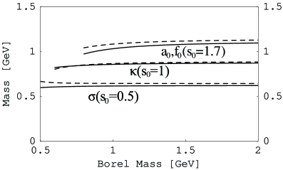
Figure 4: Masses of the $\sigma$, $\kappa$, $a_{0}$ and $f_{0}$ as tetraquark states calculated by the mixed currents $\eta_{1}$ (solid line) and $\eta_{2}$ (dashed line), as functions of the Borel mass $M_{B}$.

The current $\eta_{1}$ has the antisymmetric flavor structure and $\eta_{2}$ has the symmetric flavor structure. By using these currents with different flavor structures, we arrive at similar QCD sum rule results. This suggests that the tetraquarks of different flavor structure may mix with each other, and the tetraquark states can contain diquark and antidiquark having the mixing of the symmetric flavor $\mathbf{6_{f}}\otimes\mathbf{\bar{6}_{f}}$ and the antisymmetric flavor $\mathbf{\bar{3}_{f}}\otimes\mathbf{3_{f}}$, just like they can have a mixing of different color, spin and orbital symmetries. This is very much different from the ground baryon states, where the different flavor representations $\mathbf{8}$ and $\mathbf{10}$ correspond to different spins $\mathbf{1/2}$ and $\mathbf{3/2}$, which induces a mass splitting between $\Delta(1232)$ and $N(939)$.

V Finite Decay Width

The scalar mesons have large decay widthes, and it is important to consider their effect. In this section, we use a Gaussian distribution for the phenomenal spectral density, instead of $\delta$-function,

$$\rho^{FDW}(\sqrt{s})d\sqrt{s} \equiv \sum_{n}\langle 0|\eta|n\rangle\langle n|{\eta^{\dagger}}|0\rangle{1\over\sqrt{2\pi}\sigma}\exp\big{(}-{(\sqrt{s}-M_{n})^{2}\over 2*\sigma_{n}^{2}}\big{)}d\sqrt{s}$$ (30)

$$= {f^{2}_{X}\over\sqrt{2\pi}\sigma}\exp\big{(}-{(\sqrt{s}-M_{X})^{2}\over 2*\sigma_{X}^{2}}\big{)}d\sqrt{s}+\rm{higher\,\,states},$$

where as usual the lowest state denoted by $X$ is isolated from the rest of higher states. The Gaussian width $\sigma_{X}$ is related to the Breit-Wigner decay width $\Gamma$ by $\sigma_{X}=\Gamma/2.4$.

Again we assume the continuum contribution can be approximated by the spectral density of OPE above a threshold value $s_{0}$, and we arrive at the sum rule equation for state having a finite decay width

$$\Pi^{FDW}(M_{B}^{2})\equiv\int_{-\infty}^{+\infty}e^{-s/M_{B}^{2}}{1\over\sqrt{2\pi}\sigma}\exp\big{(}-{(\sqrt{s}-M_{X})^{2}\over 2\sigma_{X}^{2}}\big{)}d\sqrt{s}=\int^{s_{0}}_{0}e^{-s/M_{B}^{2}}\rho(s)ds\,.$$ (31)

For a given $\Gamma$, the mass can be obtained by solving the equation

$${\int_{-\infty}^{+\infty}e^{-s/M_{B}^{2}}s\exp\big{(}-{(\sqrt{s}-M_{X})^{2}\over 2\sigma_{X}^{2}}\big{)}d\sqrt{s}\over\int_{-\infty}^{+\infty}e^{-s/M_{B}^{2}}\exp\big{(}-{(\sqrt{s}-M_{X})^{2}\over 2\sigma_{X}^{2}}\big{)}d\sqrt{s}}e={\int^{s_{0}}_{0}e^{-s/M_{B}^{2}}s\rho(s)ds\over\int^{s_{0}}_{0}e^{-s/M_{B}^{2}}\rho(s)ds}\,.$$ (32)

In Fig. 5, the masses of the $\sigma(600)$, $\kappa(800)$, $a_{0}(980)$ and $f_{0}(980)$ are shown as functions of the Borel mass $M_{B}$, by setting $\Gamma=0,~{}100,~{}200$ and $400$ MeV respectively. We find that after considering the finite decay width by using the Gaussian distribution, the predicted masses do not change significantly as far as the Borel mass is within a reasonable range, where we can still reproduce the experimental data. However, the question of finite decay width is very important, and we do not consider that our attempt to use the Gaussian form is the final. We need further investigations, which we would like to put as a future important work.

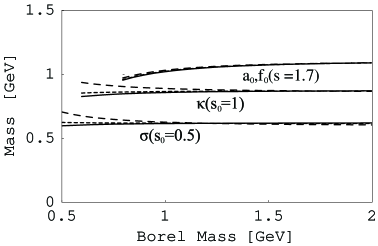
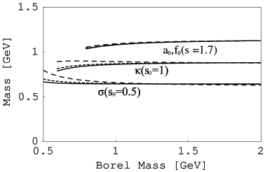
Figure 5: Masses of the $\sigma$, $\kappa$, $a_{0}$ and $f_{0}$ as tetraquark states calculated by the mixed currents $\eta_{1}$ (left) and $\eta_{2}$ (right), as functions of the Borel mass $M_{B}$. For $\sigma$ and $\kappa$, the solid, short-dashed and long-dashed curves are obtained by setting $\Gamma=0,~{}200$ and $400$ MeV respectively. For $a_{0}$ and $f_{0}$, the solid, short-dashed and long-dashed curves are obtained by setting $\Gamma=0,~{}100$ and $200$ MeV respectively.

VI Conventional $\bar{q}q$ Mesons

For comparison, we have also performed the QCD sum rule analysis using the $\bar{q}q$ current within the present framework. The QCD sum rule analyses of conventional $\bar{q}q$ mesons have been performed in Ref. Reinders:1981ww ; Kisslinger:1997gs ; Elias:1998bq ; Du:2004ki . The sum rules using the current $j=\bar{q}_{1}q_{2}$ are

$$f^{2}_{(q_{1}q_{2})}e^{-{m^{2}_{(q_{1}q_{2})}\over M_{B}^{2}}} = \int_{0}^{s_{0}}e^{-s/M_{B}^{2}}{3\over 8\pi^{2}}s\Big{(}1+{17\over 3}{\alpha_{s}\over\pi}\Big{)}ds+{3\over 2}\Big{(}m_{1}\langle\bar{q}_{2}q_{2}\rangle+m_{2}\langle\bar{q}_{1}q_{1}\rangle\Big{)}$$

$$+{1\over 8\pi}\langle{g^{2}\over 4\pi}G^{2}\rangle-{1\over 2M_{B}^{2}}\Big{(}m_{1}\langle g\bar{q}_{2}\sigma Gq_{2}\rangle+m_{2}\langle g\bar{q}_{1}\sigma Gq_{1}\rangle\Big{)}$$

$$-{16\pi\over 3M_{B}^{2}}{g_{s}\over 4\pi}{\langle\bar{q}_{1}q_{1}\rangle\langle\bar{q}_{2}q_{2}\rangle}-{16\pi\over 27M_{B}^{2}}{g_{s}\over 4\pi}\Big{(}{\langle\bar{q}_{1}q_{1}\rangle^{2}+\langle\bar{q}_{2}q_{2}\rangle}^{2}\Big{)}\,.$$

The masses of $\sigma$ and $a_{0}$ are predicted to be around 1.2 GeV, while the masses of $\kappa$ and $f_{0}$ are larger due to the $strange$ quark content. Here again we have tested other values of $M_{B}$ and $s_{0}$, and confirmed that the result shown is optimal. These results are consistent with the previous work Reinders:1981ww ; Kisslinger:1997gs ; Elias:1998bq ; Du:2004ki .

VII Summary

We have performed the QCD sum rule analysis with tetraquark currents, and found the masses of scalar mesons in the region of 600 – 1000 MeV with the ordering, $m_{\sigma}<m_{\kappa}<m_{f_{0},a_{0}}$. We have also used the conventional $\bar{q}q$ currents, and verified their masses around 1.2 GeV. We have tested all possible independent tetraquark currents as well as their linear combinations, and considered the effect of finite decay width. Our conclusions are, therefore, rather robust.

The scalar tetraquark currents can have either the antisymmetric flavor or the symmetric flavor structures. We found that there are five independent currents for each state. We investigated Borel mass $M_{B}$ and threshold value $s_{0}$ dependences, which are quite stable. The convergence of the OPE is also good, the positivity (of spectral density) is maintained, and the pole contribution is sufficient large. Therefore, we have achieved a QCD sum rule which is the best reliable within the present calculation of OPE.

Our calculation supports a tetraquark structure for low-lying scalar mesons. We find that the gluon condensate is quite large in the OPE of the mixed currents, which is related to the question of the origin of the mass generation of hadrons Weinberg:1969hw . We obtain similar results by using the currents having both the antisymmetric flavor structure and the symmetric flavor structure. This suggests that the tetraquark can have a mixing of different flavor symmetries, as well as different color, spin and orbital symmetries. There is a mass splitting due to the different flavor, color, spin and orbital structures. If this mass spitting is large enough to be observed in experiments, the tetraquark spectrum would become much more complicated; If the mass splitting is too small to be observed in experiments, a broad decay width would be observed. Such a tetraquark structure will open an alternative path toward the understanding of exotic multiquark dynamics which one does not experience in the conventional hadrons.

Appendix A Relations between $(qq)(\bar{q}\bar{q})$ and $(\bar{q}q)(\bar{q}q)$ Structures

In this appendix, we study the relations between $(qq)(\bar{q}\bar{q})$ and $(\bar{q}q)(\bar{q}q)$ currents. We work under $SU(3)_{c}\otimes~{}SU(3)_{f}\otimes~{}SO(1,3)_{L}$, where the quark field $q^{A}_{a\mu}$ has the color index $a$, flavor index $A$ and Lorentz index $\mu$. First, we consider the color and flavor structures. The interchange of both color and flavor does not need to be antisymmetric, due to the extra orbital and spin degrees of freedom. Therefore we can not use the Pauli principle such as $q^{A}_{a}q^{B}_{b}=-q^{B}_{b}q^{A}_{a}$ within the color and flavor spaces. Altogether there are four types of diquark ($qq$) and four types of quark-antiquark ($\bar{q}q$). They are shown in Table 4, where the sum over repeated indices ($a,b,\cdots$ for color indices, $A,B,\cdots$ for flavor indices) is taken.

Table 4: Color and flavor structures of $qq$ and $\bar{q}q$

(Color, Flavor)	($\mathbf{\bar{3}_{c}}$, $\mathbf{\bar{3}_{f}}$)	($\mathbf{\bar{3}_{c}}$, $\mathbf{6_{f}}$)	($\mathbf{6_{c}}$, $\mathbf{\bar{3}_{f}}$)	($\mathbf{6_{c}}$, $\mathbf{6_{f}}$)
Diquark ($qq$)	$\epsilon^{abc}\epsilon_{ABC}(q^{A}_{a}q^{B}_{b})$	$\epsilon^{abc}(q^{A}_{a}q^{B}_{b}+q^{B}_{a}q^{A}_{b})$	$\epsilon_{ABC}(q^{A}_{a}q^{B}_{b}+q^{A}_{b}q^{B}_{a})$	$(q^{A}_{a}q^{B}_{b}+q^{B}_{a}q^{A}_{b})+(a\leftrightarrow b)$
(Color, Flavor)	($\mathbf{1_{c}}$, $\mathbf{1_{f}}$)	($\mathbf{1_{c}}$, $\mathbf{8_{f}}$)	($\mathbf{8_{c}}$, $\mathbf{1_{f}}$)	($\mathbf{8_{c}}$, $\mathbf{8_{f}}$)
Quark-antiquark ($\bar{q}q$)	$(\bar{q}^{A}_{a}q^{A}_{a})$	$\lambda^{N}_{AB}(\bar{q}^{A}_{a}q^{B}_{a})$	$\lambda_{n}^{ab}(\bar{q}^{A}_{a}q^{A}_{b})$	$\lambda^{N}_{AB}\lambda_{n}^{ab}(\bar{q}^{A}_{a}q^{B}_{b})$

To construct a tetraquark by using $(qq)(\bar{q}\bar{q})$, the color is either $(\mathbf{3}\otimes\mathbf{3})\otimes(\mathbf{\bar{3}}\otimes\mathbf{\bar{3}})\rightarrow\mathbf{\bar{3}}\otimes\mathbf{3}\rightarrow\mathbf{1}$ or $(\mathbf{3}\otimes\mathbf{3})\otimes(\mathbf{\bar{3}}\otimes\mathbf{\bar{3}})\rightarrow\mathbf{6}\otimes\mathbf{\bar{6}}\rightarrow\mathbf{1}$; the flavor is $(\mathbf{3}\otimes\mathbf{3})\otimes(\mathbf{\bar{3}}\otimes\mathbf{\bar{3}})=(\mathbf{\bar{3}}\oplus\mathbf{6})\otimes(\mathbf{3}\oplus\mathbf{\bar{6}})=\mathbf{1}\oplus\mathbf{8}\oplus\mathbf{8}\oplus\mathbf{10}\oplus\mathbf{8}\oplus\mathbf{10}\oplus\mathbf{1}\oplus\mathbf{8}\oplus\mathbf{27}$; To construct a tetraquark by using $(\bar{q}q)(\bar{q}q)$, the color is either $(\mathbf{\bar{3}}\otimes\mathbf{3})\otimes(\mathbf{\bar{3}}\otimes\mathbf{3})\rightarrow\mathbf{1}\otimes\mathbf{1}\rightarrow\mathbf{1}$ or $(\mathbf{\bar{3}}\otimes\mathbf{3})\otimes(\mathbf{\bar{3}}\otimes\mathbf{3})\rightarrow\mathbf{8}\otimes\mathbf{\bar{8}}\rightarrow\mathbf{1}$, with the same flavor structure as before. In Table 5, we show all possible color and flavor structures of tetraquark currents $T^{F_{1}(F_{2})}_{C}$. Here $F_{1}$ denotes the flavor representation of tetraquark; $F_{2}$ and $C$ show the intermediate flavor and color representations of either diquark (antidiquark) or quark-antiquark. $S^{ABCD}$ is the totally symmetric matrix. Because we want to make a scalar tetraquark state, the diquark and antidiquark fields should have the same color, spin and orbital symmetries. Therefore, they must have the same flavor symmetry, which is either symmetric ($\mathbf{6_{f}}\otimes\mathbf{\bar{6}_{f}}$) or antisymmetric ($\mathbf{\bar{3}_{f}}\otimes\mathbf{3_{f}}$).

Table 5: Color and flavor structures of tetraquark currents

$(qq)(\bar{q}\bar{q})$	$(\mathbf{3}\otimes\mathbf{3})\otimes(\mathbf{\bar{3}}\otimes\mathbf{\bar{3}})\rightarrow\mathbf{\bar{3}}\otimes\mathbf{3}\rightarrow\mathbf{1_{c}}$	$(\mathbf{3}\otimes\mathbf{3})\otimes(\mathbf{\bar{3}}\otimes\mathbf{\bar{3}})\rightarrow\mathbf{6}\otimes\mathbf{\bar{6}}\rightarrow\mathbf{1_{c}}$
$(\mathbf{3}\otimes\mathbf{3})\otimes(\mathbf{\bar{3}}\otimes\mathbf{\bar{3}})$	$\epsilon^{abe}\epsilon^{cde}\epsilon_{ABE}\epsilon_{CDE}(q^{A}_{a}q^{B}_{b})(\bar{q}^{C}_{c}\bar{q}^{D}_{d})\equiv T^{\mathbf{1}(\mathbf{3})}_{\mathbf{3}}$	$\epsilon_{ABE}\epsilon_{CDE}(q^{A}_{a}q^{B}_{b}+q^{A}_{b}q^{B}_{a})(\bar{q}^{C}_{a}\bar{q}^{D}_{b}+\bar{q}^{C}_{b}\bar{q}^{D}_{a})$
$\rightarrow\mathbf{\bar{3}}\otimes\mathbf{3}\rightarrow\mathbf{1_{f}}$		$=2\epsilon_{ABE}\epsilon_{CDE}(q^{A}_{a}q^{B}_{b})(\bar{q}^{C}_{a}\bar{q}^{D}_{b}+\bar{q}^{C}_{b}\bar{q}^{D}_{a})\equiv 2T^{\mathbf{1}(\mathbf{3})}_{\mathbf{6}}$
$\rightarrow\mathbf{\bar{3}}\otimes\mathbf{3}\rightarrow\mathbf{8_{f}}$	$\epsilon^{abe}\epsilon^{cde}\lambda_{N}^{EF}\epsilon_{ABE}\epsilon_{CDF}(q^{A}_{a}q^{B}_{b})(\bar{q}^{C}_{c}\bar{q}^{D}_{d})\equiv T^{\mathbf{8}(\mathbf{3})}_{\mathbf{3}}$	$\lambda_{N}^{EF}\epsilon_{ABE}\epsilon_{CDF}(q^{A}_{a}q^{B}_{b})(\bar{q}^{C}_{a}\bar{q}^{D}_{b}+\bar{q}^{C}_{b}\bar{q}^{D}_{a})\equiv T^{\mathbf{8}(\mathbf{3})}_{\mathbf{6}}$
$\rightarrow\mathbf{\bar{3}}\otimes\mathbf{\bar{6}}\rightarrow\mathbf{8_{f}}$	$\epsilon^{abe}\epsilon^{cde}\lambda_{N}^{DF}\epsilon_{ABE}\epsilon_{CEF}(q^{A}_{a}q^{B}_{b})(\bar{q}^{C}_{c}\bar{q}^{D}_{d})\equiv T^{\mathbf{8}(\mathbf{3},\mathbf{6})}_{\mathbf{3}}$	$\lambda_{N}^{DF}\epsilon_{ABE}\epsilon_{CEF}(q^{A}_{a}q^{B}_{b})(\bar{q}^{C}_{a}\bar{q}^{D}_{b}+\bar{q}^{C}_{b}\bar{q}^{D}_{a})\equiv T^{\mathbf{8}(\mathbf{3},\mathbf{6})}_{\mathbf{6}}$
$\rightarrow\mathbf{\bar{3}}\otimes\mathbf{\bar{6}}\rightarrow\mathbf{10_{f}}$	$\epsilon^{abe}\epsilon^{cde}S^{CDE}\epsilon_{ABE}(q^{A}_{a}q^{B}_{b})(\bar{q}^{C}_{c}\bar{q}^{D}_{d})\equiv T^{\mathbf{10}(\mathbf{3},\mathbf{6})}_{\mathbf{3}}$	$S^{CDE}\epsilon_{ABE}(q^{A}_{a}q^{B}_{b})(\bar{q}^{C}_{a}\bar{q}^{D}_{b}+\bar{q}^{C}_{b}\bar{q}^{D}_{a})\equiv T^{\mathbf{10}(\mathbf{3},\mathbf{6})}_{\mathbf{6}}$
$\rightarrow\mathbf{6}\otimes\mathbf{3}\rightarrow\mathbf{8_{f}}$	$\epsilon^{abe}\epsilon^{cde}\lambda_{N}^{BF}\epsilon_{AEF}\epsilon_{CDE}(q^{A}_{a}q^{B}_{b})(\bar{q}^{C}_{c}\bar{q}^{D}_{d})\equiv T^{\mathbf{8}(\mathbf{6},\mathbf{3})}_{\mathbf{3}}$	$\lambda_{N}^{BF}\epsilon_{AEF}\epsilon_{CDE}(q^{A}_{a}q^{B}_{b})(\bar{q}^{C}_{a}\bar{q}^{D}_{b}+\bar{q}^{C}_{b}\bar{q}^{D}_{a})\equiv T^{\mathbf{8}(\mathbf{6},\mathbf{3})}_{\mathbf{6}}$
$\rightarrow\mathbf{6}\otimes\mathbf{3}\rightarrow\mathbf{10_{f}}$	$\epsilon^{abe}\epsilon^{cde}S^{ABE}\epsilon_{CDE}(q^{A}_{a}q^{B}_{b})(\bar{q}^{C}_{c}\bar{q}^{D}_{d})\equiv T^{\mathbf{10}(\mathbf{6},\mathbf{3})}_{\mathbf{3}}$	$S^{ABE}\epsilon_{CDE}(q^{A}_{a}q^{B}_{b})(\bar{q}^{C}_{a}\bar{q}^{D}_{b}+\bar{q}^{C}_{b}\bar{q}^{D}_{a})\equiv T^{\mathbf{10}(\mathbf{6},\mathbf{3})}_{\mathbf{6}}$
$\rightarrow\mathbf{6}\otimes\mathbf{\bar{6}}\rightarrow\mathbf{1_{f}}$	$\epsilon^{abe}\epsilon^{cde}(q^{A}_{a}q^{B}_{b}+q^{B}_{a}q^{A}_{b})(\bar{q}^{A}_{c}\bar{q}^{B}_{d}+\bar{q}^{B}_{c}\bar{q}^{A}_{d})$	$(q^{A}_{a}q^{B}_{b}+q^{B}_{a}q^{A}_{b})(\bar{q}^{A}_{a}\bar{q}^{B}_{b}+\bar{q}^{B}_{a}\bar{q}^{A}_{b}+(a\leftrightarrow b))$
	$=2\epsilon^{abe}\epsilon^{cde}(q^{A}_{a}q^{B}_{b})(\bar{q}^{A}_{c}\bar{q}^{B}_{d}+\bar{q}^{B}_{c}\bar{q}^{A}_{d})\equiv 2T^{\mathbf{1}(\mathbf{6})}_{\mathbf{3}}$	$=2(q^{A}_{a}q^{B}_{b})(\bar{q}^{A}_{a}\bar{q}^{B}_{b}+\bar{q}^{B}_{a}\bar{q}^{A}_{b}+(a\leftrightarrow b))\equiv 2T^{\mathbf{1}(\mathbf{6})}_{\mathbf{6}}$
$\rightarrow\mathbf{6}\otimes\mathbf{\bar{6}}\rightarrow\mathbf{8_{f}}$	$\lambda^{N}_{BC}\epsilon^{abe}\epsilon^{cde}(q^{A}_{a}q^{B}_{b}+q^{B}_{a}q^{A}_{b})(\bar{q}^{A}_{c}\bar{q}^{C}_{d}+\bar{q}^{C}_{c}\bar{q}^{A}_{d})\equiv T^{\mathbf{8}(\mathbf{6})}_{\mathbf{3}}$	$\lambda^{N}_{BC}(q^{A}_{a}q^{B}_{b}+q^{B}_{a}q^{A}_{b})(\bar{q}^{A}_{a}\bar{q}^{C}_{b}+\bar{q}^{C}_{a}\bar{q}^{A}_{b}+(a\leftrightarrow b))\equiv T^{\mathbf{8}(\mathbf{6})}_{\mathbf{6}}$
$\rightarrow\mathbf{6}\otimes\mathbf{\bar{6}}\rightarrow\mathbf{27_{f}}$	$S_{ABCD}\epsilon^{abe}\epsilon^{cde}(q^{A}_{a}q^{B}_{b})(\bar{q}^{C}_{c}\bar{q}^{D}_{d})\equiv T^{\mathbf{27}(\mathbf{6})}_{\mathbf{3}}$	$S_{ABCD}(q^{A}_{a}q^{B}_{b})(\bar{q}^{C}_{a}\bar{q}^{D}_{b}+\bar{q}^{C}_{b}\bar{q}^{D}_{a})\equiv T^{\mathbf{27}(\mathbf{6})}_{\mathbf{6}}$
$(\bar{q}q)(\bar{q}q)$	$(\mathbf{\bar{3}}\otimes\mathbf{3})\otimes(\mathbf{\bar{3}}\otimes\mathbf{3})\rightarrow\mathbf{1}\otimes\mathbf{1}\rightarrow\mathbf{1_{c}}$	$(\mathbf{\bar{3}}\otimes\mathbf{3})\otimes(\mathbf{\bar{3}}\otimes\mathbf{3})\rightarrow\mathbf{8}\otimes\mathbf{8}\rightarrow\mathbf{1_{c}}$
$(\mathbf{\bar{3}}\otimes\mathbf{3})\otimes(\mathbf{\bar{3}}\otimes\mathbf{3})$	$(\bar{q}^{A}_{a}q^{A}_{a})(\bar{q}^{B}_{b}q^{B}_{b})\equiv T^{\mathbf{1}(\mathbf{1})}_{\mathbf{1}}$	$(\bar{q}^{A}_{a}\lambda_{n}^{ab}q^{A}_{b})(\bar{q}^{B}_{c}\lambda_{n}^{cd}q^{B}_{d})\equiv T^{\mathbf{1}(\mathbf{1})}_{\mathbf{8}}$
$\rightarrow\mathbf{1}\otimes\mathbf{1}\rightarrow\mathbf{1_{f}}$
$\rightarrow\mathbf{1}\otimes\mathbf{8}\rightarrow\mathbf{8_{f}}$	$\lambda^{N}_{BC}(\bar{q}^{A}_{a}q^{A}_{a})(\bar{q}^{B}_{b}q^{C}_{b})\equiv T^{\mathbf{8}(\mathbf{1},~{}\mathbf{8})}_{\mathbf{1}}$	$\lambda^{N}_{BC}(\bar{q}^{A}_{a}\lambda_{n}^{ab}q^{A}_{b})(\bar{q}^{B}_{c}\lambda_{n}^{cd}q^{C}_{d})\equiv T^{\mathbf{8}(\mathbf{1},~{}\mathbf{8})}_{\mathbf{8}}$
$\rightarrow\mathbf{8}\otimes\mathbf{1}\rightarrow\mathbf{8_{f}}$	$\lambda^{N}_{BC}(\bar{q}^{B}_{a}q^{C}_{a})(\bar{q}^{A}_{b}q^{A}_{b})\equiv T^{\mathbf{8}(\mathbf{8},~{}\mathbf{1})}_{\mathbf{1}}$	$\lambda^{N}_{BC}(\bar{q}^{B}_{a}\lambda_{n}^{ab}q^{C}_{b})(\bar{q}^{A}_{c}\lambda_{n}^{cd}q^{A}_{d})\equiv T^{\mathbf{8}(\mathbf{8},~{}\mathbf{1})}_{\mathbf{8}}$
$\rightarrow\mathbf{8}\otimes\mathbf{8}\rightarrow\mathbf{1_{f}}$	$(\bar{q}^{A}_{a}\lambda^{N}_{AB}q^{B}_{a})(\bar{q}^{C}_{b}\lambda^{N}_{CD}q^{D}_{b})\equiv T^{\mathbf{1}(\mathbf{8})}_{\mathbf{1}}$	$(\bar{q}^{A}_{a}\lambda_{n}^{ab}\lambda^{N}_{AB}q^{B}_{b})(\bar{q}^{C}_{c}\lambda_{n}^{cd}\lambda^{N}_{CD}q^{D}_{d})\equiv T^{\mathbf{1}(\mathbf{8})}_{\mathbf{8}}$
$\rightarrow\mathbf{8}\otimes\mathbf{8}\rightarrow\mathbf{8_{f}}$	$\lambda_{N}^{FE}\epsilon_{ACE}\epsilon_{BDF}(\bar{q}^{A}_{a}q^{B}_{a})(\bar{q}^{C}_{b}q^{D}_{b})\equiv T^{\mathbf{8}(\mathbf{8})}_{\mathbf{1}}$	$\lambda_{N}^{FE}\epsilon_{ACE}\epsilon_{BDF}(\bar{q}^{A}_{a}\lambda_{n}^{ab}q^{B}_{b})(\bar{q}^{C}_{c}\lambda_{n}^{cd}q^{D}_{d})\equiv T^{\mathbf{8}(\mathbf{8})}_{\mathbf{8}}$
$\rightarrow\mathbf{8}\otimes\mathbf{8}\rightarrow\mathbf{8_{f}^{\prime}}$	$\lambda_{N}^{BF}\epsilon_{ACE}\epsilon_{DEF}(\bar{q}^{A}_{a}q^{B}_{a})(\bar{q}^{C}_{b}q^{D}_{b})\equiv T^{\mathbf{8^{\prime}}(\mathbf{8})}_{\mathbf{1}}$	$\lambda_{N}^{BF}\epsilon_{ACE}\epsilon_{DEF}(\bar{q}^{A}_{a}\lambda_{n}^{ab}q^{B}_{b})(\bar{q}^{C}_{c}\lambda_{n}^{cd}q^{D}_{d})\equiv T^{\mathbf{8^{\prime}}(\mathbf{8})}_{\mathbf{8}}$
$\rightarrow\mathbf{8}\otimes\mathbf{8}\rightarrow\mathbf{10_{f}}$	$\epsilon_{ACE}S_{BDE}(\bar{q}^{A}_{a}q^{B}_{a})(\bar{q}^{C}_{b}q^{D}_{b})\equiv T^{\mathbf{10}(\mathbf{8})}_{\mathbf{1}}$	$\epsilon_{ACE}S_{BDE}(\bar{q}^{A}_{a}\lambda_{n}^{ab}q^{B}_{b})(\bar{q}^{C}_{c}\lambda_{n}^{cd}q^{D}_{d})\equiv T^{\mathbf{10}(\mathbf{8})}_{\mathbf{8}}$
$\rightarrow\mathbf{8}\otimes\mathbf{8}\rightarrow\mathbf{10_{f}^{\prime}}$	$\epsilon_{BDE}S_{ACE}(\bar{q}^{A}_{a}q^{B}_{a})(\bar{q}^{C}_{b}q^{D}_{b})\equiv T^{\mathbf{10^{\prime}}(\mathbf{8})}_{\mathbf{1}}$	$\epsilon_{BDE}S_{ACE}(\bar{q}^{A}_{a}\lambda_{n}^{ab}q^{B}_{b})(\bar{q}^{C}_{c}\lambda_{n}^{cd}q^{D}_{d})\equiv T^{\mathbf{10^{\prime}}(\mathbf{8})}_{\mathbf{8}}$
$\rightarrow\mathbf{8}\otimes\mathbf{8}\rightarrow\mathbf{27_{f}}$	$S_{ABCD}(\bar{q}^{A}_{a}q^{B}_{a})(\bar{q}^{C}_{b}q^{D}_{b})\equiv T^{\mathbf{27}(\mathbf{8})}_{\mathbf{1}}$	$S_{ABCD}(\bar{q}^{A}_{a}\lambda_{n}^{ab}q^{B}_{b})(\bar{q}^{C}_{c}\lambda_{n}^{cd}q^{D}_{d})\equiv T^{\mathbf{27}(\mathbf{8})}_{\mathbf{8}}$

If the orbital and spin structure between the two quarks (two antiquarks) are symmetric, then the color-flavor structure of diquark (antidiquark) should be anti-symmetric, which means $q^{A}_{a}q^{B}_{b}=-q^{B}_{b}q^{A}_{a}$ ($\bar{q}^{A}_{a}\bar{q}^{B}_{b}=-\bar{q}^{B}_{b}\bar{q}^{A}_{a}$). In this case, we can verify

$$T^{\mathbf{1}(\mathbf{3})}_{\mathbf{3}}=T^{\mathbf{8}(\mathbf{3})}_{\mathbf{3}}=T^{\mathbf{8}(\mathbf{3},\mathbf{6})}_{\mathbf{3}}=T^{\mathbf{10}(\mathbf{3},\mathbf{6})}_{\mathbf{3}}=T^{\mathbf{8}(\mathbf{6},\mathbf{3})}_{\mathbf{6}}=T^{\mathbf{10}(\mathbf{6},\mathbf{3})}_{\mathbf{6}}=T^{\mathbf{1}(\mathbf{6})}_{\mathbf{6}}=T^{\mathbf{8}(\mathbf{6})}_{\mathbf{6}}=T^{\mathbf{27}(\mathbf{6})}_{\mathbf{6}}=0\,,$$ (34)

If the orbital and spin structure between two quarks (two antiquarks) are anti-symmetric, then the color-flavor structure of diquark (antidiquark) should be symmetric, which means $q^{A}_{a}q^{B}_{b}=q^{B}_{b}q^{A}_{a}$ ($\bar{q}^{A}_{a}\bar{q}^{B}_{b}=\bar{q}^{B}_{b}\bar{q}^{A}_{a}$). Then we can verify

$$T^{\mathbf{1}(\mathbf{3})}_{\mathbf{6}}=T^{\mathbf{8}(\mathbf{3})}_{\mathbf{6}}=T^{\mathbf{8}(\mathbf{3},\mathbf{6})}_{\mathbf{6}}=T^{\mathbf{10}(\mathbf{3},\mathbf{6})}_{\mathbf{6}}=T^{\mathbf{8}(\mathbf{6},\mathbf{3})}_{\mathbf{3}}=T^{\mathbf{10}(\mathbf{6},\mathbf{3})}_{\mathbf{3}}=T^{\mathbf{1}(\mathbf{6})}_{\mathbf{3}}=T^{\mathbf{8}(\mathbf{6})}_{\mathbf{3}}=T^{\mathbf{27}(\mathbf{6})}_{\mathbf{3}}=0\,.$$ (35)

Now let us discuss the Fierz rearrangement in order to relate $(qq)(\bar{q}\bar{q})$ and $(\bar{q}q)(\bar{q}q)$ structures. First we perform it in the color and flavor spaces. To do this, it is convenient to consider the interchange of color indices:

$$(q^{A}_{a}q^{B}_{b}\bar{q}^{C}_{a}\bar{q}^{D}_{b})={1\over 3}(q^{A}_{a}q^{B}_{b}\bar{q}^{C}_{b}\bar{q}^{D}_{a})+{1\over 2}\lambda_{n}^{ab}\lambda_{n}^{cd}(q^{A}_{a}q^{B}_{c}\bar{q}^{C}_{d}\bar{q}^{D}_{b})\,,$$

$$\lambda_{n}^{ab}\lambda_{n}^{cd}(q^{A}_{a}q^{B}_{c}\bar{q}^{C}_{b}\bar{q}^{D}_{d})={16\over 9}(q^{A}_{a}q^{B}_{b}\bar{q}^{C}_{b}\bar{q}^{D}_{a})-{1\over 3}\lambda_{n}^{ab}\lambda_{n}^{cd}(q^{A}_{a}q^{B}_{c}\bar{q}^{C}_{d}\bar{q}^{D}_{b})\,.$$ (36)

We can obtain the same result for flavor structure.

Let us take $T^{\mathbf{1}(\mathbf{3})}_{\mathbf{3}}$ as an example, and perform the simultaneous interchange of both color and flavor indices

$$T^{\mathbf{1}(\mathbf{3})}_{\mathbf{3}} = \epsilon^{abe}\epsilon^{cde}\epsilon_{ABE}\epsilon_{CDE}(q^{A}_{a}q^{B}_{b})(\bar{q}^{C}_{c}\bar{q}^{D}_{d})$$

$$= (q^{A}_{a}q^{B}_{b})(\bar{q}^{A}_{a}\bar{q}^{B}_{b})-(q^{A}_{a}q^{B}_{b})(\bar{q}^{A}_{b}\bar{q}^{B}_{a})-(q^{A}_{a}q^{B}_{b})(\bar{q}^{B}_{a}\bar{q}^{A}_{b})+(q^{A}_{a}q^{B}_{b})(\bar{q}^{B}_{b}\bar{q}^{A}_{a})$$

$$= (q^{A}_{a}q^{B}_{b})(\bar{q}^{A}_{a}\bar{q}^{B}_{b})-\Big{(}{1\over 3}(q^{A}_{a}q^{B}_{b})(\bar{q}^{A}_{a}\bar{q}^{B}_{b})+{1\over 2}\lambda_{n}^{ab}\lambda_{n}^{cd}(q^{A}_{a}q^{B}_{c})(\bar{q}^{A}_{b}\bar{q}^{B}_{d})\Big{)}$$

$$-(q^{A}_{a}q^{B}_{b})(\bar{q}^{B}_{a}\bar{q}^{A}_{b})+\Big{(}{1\over 3}(q^{A}_{a}q^{B}_{b})(\bar{q}^{B}_{a}\bar{q}^{A}_{b})+{1\over 2}\lambda_{n}^{ab}\lambda_{n}^{cd}(q^{A}_{a}q^{B}_{c})(\bar{q}^{B}_{b}\bar{q}^{A}_{d})\Big{)}$$

$$= {2\over 3}(q^{A}_{a}q^{B}_{b})(\bar{q}^{A}_{a}\bar{q}^{B}_{b})-{1\over 2}\lambda_{n}^{ab}\lambda_{n}^{cd}(q^{A}_{a}q^{B}_{c})(\bar{q}^{A}_{b}\bar{q}^{B}_{d})-{2\over 3}\Big{(}{1\over 3}(q^{A}_{a}q^{B}_{b})(\bar{q}^{A}_{a}\bar{q}^{B}_{b})+{1\over 2}\lambda^{N}_{AB}\lambda^{N}_{CD}(q^{A}_{a}q^{C}_{b})(\bar{q}^{B}_{a}\bar{q}^{D}_{b})\Big{)}$$

$$+{1\over 2}\Big{(}{1\over 3}\lambda_{n}^{ab}\lambda_{n}^{cd}(q^{A}_{a}q^{B}_{c})(\bar{q}^{A}_{b}\bar{q}^{B}_{d})+{1\over 2}\lambda^{N}_{AB}\lambda^{N}_{CD}\lambda_{n}^{ab}\lambda_{n}^{cd}(q^{A}_{a}q^{C}_{c})(\bar{q}^{B}_{b}\bar{q}^{D}_{d})\Big{)}$$

$$= {4\over 9}(q^{A}_{a}q^{B}_{b})(\bar{q}^{A}_{a}\bar{q}^{B}_{b})-{1\over 3}\lambda_{n}^{ab}\lambda_{n}^{cd}(q^{A}_{a}q^{B}_{c})(\bar{q}^{A}_{b}\bar{q}^{B}_{d})-{1\over 3}\lambda^{N}_{AB}\lambda^{N}_{CD}(q^{A}_{a}q^{C}_{b})(\bar{q}^{B}_{a}\bar{q}^{D}_{b})$$

$$+{1\over 4}\lambda^{N}_{AB}\lambda^{N}_{CD}\lambda_{n}^{ab}\lambda_{n}^{cd}(q^{A}_{a}q^{C}_{c})(\bar{q}^{B}_{b}\bar{q}^{D}_{d})\,.$$

Because we only consider the color and flavor structures, by changing the ordering of the second quark and third quark, we arrive at the result:

$$\sim {4\over 9}(\bar{q}^{A}_{a}q^{A}_{a})(\bar{q}^{B}_{b}q^{B}_{b})-{1\over 3}\lambda_{n}^{ab}\lambda_{n}^{cd}(\bar{q}^{A}_{b}q^{A}_{a})(\bar{q}^{B}_{d}q^{B}_{c})-{1\over 3}\lambda^{N}_{AB}\lambda^{N}_{CD}(\bar{q}^{B}_{a}q^{A}_{a})(\bar{q}^{D}_{b}q^{C}_{b})$$ (37)

$$+{1\over 4}\lambda^{N}_{AB}\lambda^{N}_{CD}\lambda_{n}^{ab}\lambda_{n}^{cd}(\bar{q}^{B}_{b}q^{A}_{a})(\bar{q}^{D}_{d}q^{C}_{c})\,.$$

$$= {4\over 9}T^{\mathbf{1}(\mathbf{1})}_{\mathbf{1}}-{1\over 3}T^{\mathbf{1}(\mathbf{1})}_{\mathbf{8}}-{1\over 3}T^{\mathbf{1}(\mathbf{8})}_{\mathbf{1}}+{1\over 4}T^{\mathbf{1}(\mathbf{8})}_{\mathbf{8}}\,.$$

Next we perform the Fierz rearrangement in the Lorentz indices. The formulae is:

$$(\mathbf{1})_{\alpha\beta}(\mathbf{1})_{\gamma\delta}={1\over 4}(\mathbf{1})_{\alpha\delta}(\mathbf{1})_{\gamma\beta}+{1\over 4}(\mathbf{\gamma_{\mu}})_{\alpha\delta}(\mathbf{\gamma^{\mu}})_{\gamma\beta}+{1\over 8}(\mathbf{\sigma_{\mu\nu}})_{\alpha\delta}(\mathbf{\sigma^{\mu\nu}})_{\gamma\beta}-{1\over 4}(\mathbf{\gamma_{\mu}\gamma_{5}})_{\alpha\delta}(\mathbf{\gamma^{\mu}\gamma_{5}})_{\gamma\beta}+{1\over 4}(\mathbf{\gamma_{5}})_{\alpha\delta}(\mathbf{\gamma_{5}})_{\gamma\beta}\,.$$ (38)

By using this equation, we can obtain various relations such as

$$((q^{A}_{a})^{T}Cq^{B}_{b})(\bar{q}^{C}_{c}C(\bar{q}^{D}_{d})^{T}) = -{1\over 4}((q^{A}_{a})^{T}CC(\bar{q}^{D}_{d})^{T})(\bar{q}^{C}_{c}q^{B}_{b})-{1\over 4}((q^{A}_{a})^{T}C\gamma_{\mu}C(\bar{q}^{D}_{d})^{T})(\bar{q}^{C}_{c}\gamma^{\mu}q^{B}_{b})$$ (39)

$$-{1\over 8}((q^{A}_{a})^{T}C\sigma_{\mu\nu}C(\bar{q}^{D}_{d})^{T})(\bar{q}^{C}_{c}\sigma^{\mu\nu}q^{B}_{b})+{1\over 4}((q^{A}_{a})^{T}C\gamma_{\mu}\gamma_{5}C(\bar{q}^{D}_{d})^{T})(\bar{q}^{C}_{c}\gamma^{\mu}\gamma_{5}q^{B}_{b})$$

$$-{1\over 4}((q^{A}_{a})^{T}C\gamma_{5}C(\bar{q}^{D}_{d})^{T})(\bar{q}^{C}_{c}\gamma_{5}q^{B}_{b})$$

$$= -{1\over 4}(\bar{q}^{D}_{d}q^{A}_{a})(\bar{q}^{C}_{c}q^{B}_{b})+{1\over 4}(\bar{q}^{D}_{d}\gamma_{\mu}q^{A}_{a})(\bar{q}^{C}_{c}\gamma^{\mu}q^{B}_{b})+{1\over 8}(\bar{q}^{D}_{d}\sigma_{\mu\nu}q^{A}_{a})(\bar{q}^{C}_{c}\sigma^{\mu\nu}q^{B}_{b})$$

$$+{1\over 4}(\bar{q}^{D}_{d}\gamma_{\mu}\gamma_{5}q^{A}_{a})(\bar{q}^{C}_{c}\gamma^{\mu}\gamma_{5}q^{B}_{b})-{1\over 4}(\bar{q}^{D}_{d}\gamma_{5}q^{A}_{a})(\bar{q}^{C}_{c}\gamma_{5}q^{B}_{b})\,.$$

In order to label the Lorentz structure for a scalar tetraquark field, we introduce $S$, $V$, $T$, $A$ and $P$ instead of $T$:

$$S\mbox{ for }(q^{T}C\gamma_{5}q)(\bar{q}\gamma_{5}C\bar{q}^{T})\mbox{ and }(\bar{q}q)(\bar{q}q)\,,$$

$$V\mbox{ for }(q^{T}C\gamma_{\mu}\gamma_{5}q)(\bar{q}\gamma^{\mu}\gamma_{5}C\bar{q}^{T})\mbox{ and }(\bar{q}\gamma_{\mu}q)(\bar{q}\gamma^{\mu}q)\,,$$

$$T\mbox{ for }(q^{T}C\sigma_{\mu\nu}q)(\bar{q}\sigma^{\mu\nu}C\bar{q}^{T})\mbox{ and }(\bar{q}\sigma_{\mu\nu}q)(\bar{q}\sigma^{\mu\nu}q)\,,$$

$$A\mbox{ for }(q^{T}C\gamma_{\mu}q)(\bar{q}\gamma^{\mu}C\bar{q}^{T})\mbox{ and }(\bar{q}\gamma_{\mu}\gamma_{5}q)(\bar{q}\gamma^{\mu}\gamma_{5}q)\,,$$

$$P\mbox{ for }(q^{T}Cq)(\bar{q}C\bar{q}^{T})\mbox{ and }(\bar{q}\gamma_{5}q)(\bar{q}\gamma_{5}q)\,.$$

For example,

$$S^{\mathbf{27}(\mathbf{6})}_{\mathbf{6}}\equiv S_{ABCD}(q^{AT}_{a}C\gamma_{5}q^{B}_{b})(\bar{q}^{C}_{a}\gamma_{5}C\bar{q}^{DT}_{b}+\bar{q}^{C}_{b}\gamma_{5}C\bar{q}^{DT}_{a})\,,$$

$$V^{\mathbf{27}(\mathbf{8})}_{\mathbf{1}}\equiv S_{ABCD}(\bar{q}^{A}_{a}\gamma_{\mu}q^{B}_{a})(\bar{q}^{C}_{b}\gamma^{\mu}q^{D}_{b})\,.$$ (40)

Diquarks belonging to $T$ and $A$ have a symmetric Lorentz structure (see Eq. 34)

$$(C\gamma_{\mu})_{\alpha\beta}=(C\gamma_{\mu})_{\beta\alpha}\,,(C\sigma_{\mu\nu})_{\alpha\beta}=(C\sigma_{\mu\nu})_{\beta\alpha}\,,$$ (41)

so they have an anti-symmetric color-flavor structure. Therefore, currents having the symmetric color-flavor structure vanish, such as

$$A^{\mathbf{1}(\mathbf{3})}_{\mathbf{3}}=\epsilon^{abe}\epsilon^{cde}\epsilon_{ABE}\epsilon_{CDE}((q^{A}_{a})^{T}C\gamma_{\mu}q^{B}_{b})(\bar{q}^{C}_{c}\gamma^{\mu}C(\bar{q}^{D}_{d})^{T})=0\,.$$ (42)

Similarly, diquarks belonging to $S$, $V$ and $P$ have an anti-symmetric Lorentz structure (see Eq. 35)

$$(C)_{\alpha\beta}=-(C)_{\beta\alpha}\,,(C\gamma_{\mu}\gamma_{5})_{\alpha\beta}=-(C\gamma_{\mu}\gamma_{5})_{\beta\alpha}\,,(C\gamma_{5})_{\alpha\beta}=-(C\gamma_{5})_{\beta\alpha}\,,$$ (43)

and so they have a symmetric color-flavor structure.

By now, we have known the flavor, color and Lorentz structures of scalar tetraquark fields, for both $(qq)(\bar{q}\bar{q})$ and $(\bar{q}q)(\bar{q}q)$ structures, and are ready to derive some relations.

A.1 Specifying the flavor structure

In order to establish the relations, we need to specify the flavor quantum numbers of the tetraquark currents. As we are considering in this work, let us choose the flavor octet states $(\mathbf{3}\otimes\mathbf{3})\otimes(\mathbf{\bar{3}}\otimes\mathbf{\bar{3}})\rightarrow\mathbf{\bar{3}}\otimes\mathbf{3}\rightarrow\mathbf{8_{f}}$ for the illustration.

In this case, diquarks and antidiquarks have an anti-symmetric flavor structure, and we can verify

$$S^{\mathbf{8}(\mathbf{3})}_{\mathbf{6}}=V^{\mathbf{8}(\mathbf{3})}_{\mathbf{6}}=T^{\mathbf{8}(\mathbf{3})}_{\mathbf{3}}=A^{\mathbf{8}(\mathbf{3})}_{\mathbf{3}}=P^{\mathbf{8}(\mathbf{3})}_{\mathbf{6}}=0\,.$$ (44)

Therefore, there are five types of $(qq)(\bar{q}\bar{q})$ fields which are non-zero and independent:

$$S^{\mathbf{8}(\mathbf{3})}_{\mathbf{3}}\,,V^{\mathbf{8}(\mathbf{3})}_{\mathbf{3}}\,,T^{\mathbf{8}(\mathbf{3})}_{\mathbf{6}}\,,A^{\mathbf{8}(\mathbf{3})}_{\mathbf{6}}\,,P^{\mathbf{8}(\mathbf{3})}_{\mathbf{3}}\,,$$

while all ten types remain for the $(\bar{q}q)(\bar{q}q)$ fields:

$$S^{\mathbf{8}(\mathbf{8})}_{\mathbf{1}}\,,V^{\mathbf{8}(\mathbf{8})}_{\mathbf{1}}\,,T^{\mathbf{8}(\mathbf{8})}_{\mathbf{1}}\,,A^{\mathbf{8}(\mathbf{8})}_{\mathbf{1}}\,,P^{\mathbf{8}(\mathbf{8})}_{\mathbf{1}}\,,S^{\mathbf{8}(\mathbf{8})}_{\mathbf{8}}\,,V^{\mathbf{8}(\mathbf{8})}_{\mathbf{8}}\,,T^{\mathbf{8}(\mathbf{8})}_{\mathbf{8}}\,,A^{\mathbf{8}(\mathbf{8})}_{\mathbf{8}}\,,P^{\mathbf{8}(\mathbf{8})}_{\mathbf{8}}\,,$$

Among these ten $(\bar{q}q)(\bar{q}q)$ fields, only five are independent. We can derive the following five equation by applying the Fierz transformation for the $(\bar{q}q)(\bar{q}q)$ fields:

$$S^{\mathbf{8}(\mathbf{8})}_{\mathbf{8}} = -\frac{1}{6}S^{\mathbf{8}(\mathbf{8})}_{\mathbf{1}}+\frac{1}{2}V^{\mathbf{8}(\mathbf{8})}_{\mathbf{1}}+\frac{1}{4}T^{\mathbf{8}(\mathbf{8})}_{\mathbf{1}}-\frac{1}{2}A^{\mathbf{8}(\mathbf{8})}_{\mathbf{1}}-\frac{1}{2}P^{\mathbf{8}(\mathbf{8})}_{\mathbf{1}}\,,$$

$$V^{\mathbf{8}(\mathbf{8})}_{\mathbf{8}} = 2S^{\mathbf{8}(\mathbf{8})}_{\mathbf{1}}-\frac{5}{3}V^{\mathbf{8}(\mathbf{8})}_{\mathbf{1}}-A^{\mathbf{8}(\mathbf{8})}_{\mathbf{1}}-2P^{\mathbf{8}(\mathbf{8})}_{\mathbf{1}}\,,$$

$$T^{\mathbf{8}(\mathbf{8})}_{\mathbf{8}} = 6S^{\mathbf{8}(\mathbf{8})}_{\mathbf{1}}-\frac{5}{3}T^{\mathbf{8}(\mathbf{8})}_{\mathbf{1}}+6P^{\mathbf{8}(\mathbf{8})}_{\mathbf{1}}\,,$$ (45)

$$A^{\mathbf{8}(\mathbf{8})}_{\mathbf{8}} = -2S^{\mathbf{8}(\mathbf{8})}_{\mathbf{1}}-V^{\mathbf{8}(\mathbf{8})}_{\mathbf{1}}-\frac{5}{3}A^{\mathbf{8}(\mathbf{8})}_{\mathbf{1}}+2P^{\mathbf{8}(\mathbf{8})}_{\mathbf{1}}\,,$$

$$P^{\mathbf{8}(\mathbf{8})}_{\mathbf{8}} = \frac{1}{2}S^{\mathbf{8}(\mathbf{8})}_{\mathbf{1}}-\frac{1}{2}V^{\mathbf{8}(\mathbf{8})}_{\mathbf{1}}+\frac{1}{4}T^{\mathbf{8}(\mathbf{8})}_{\mathbf{1}}+\frac{1}{2}A^{\mathbf{8}(\mathbf{8})}_{\mathbf{1}}-\frac{1}{6}P^{\mathbf{8}(\mathbf{8})}_{\mathbf{1}}\,.$$

Employing the five currents on the left hand sides of Eqs. (A.1) as independent ones, and applying the Fierz transformation, we can establish the following relations among the five $(qq)(\bar{q}\bar{q})$ and five $(\bar{q}q)(\bar{q}q)$ structures:

$$S^{\mathbf{8}(\mathbf{3})}_{\mathbf{3}} = -\frac{1}{2}S^{\mathbf{8}(\mathbf{8})}_{\mathbf{1}}-\frac{1}{2}V^{\mathbf{8}(\mathbf{8})}_{\mathbf{1}}+\frac{1}{4}T^{\mathbf{8}(\mathbf{8})}_{\mathbf{1}}-\frac{1}{2}A^{\mathbf{8}(\mathbf{8})}_{\mathbf{1}}-\frac{1}{2}P^{\mathbf{8}(\mathbf{8})}_{\mathbf{1}}\,,$$

$$V^{\mathbf{8}(\mathbf{3})}_{\mathbf{3}} = 2S^{\mathbf{8}(\mathbf{8})}_{\mathbf{1}}-V^{\mathbf{8}(\mathbf{8})}_{\mathbf{1}}+A^{\mathbf{8}(\mathbf{8})}_{\mathbf{1}}-2P^{\mathbf{8}(\mathbf{8})}_{\mathbf{1}}\,,$$

$$T^{\mathbf{8}(\mathbf{3})}_{\mathbf{6}} = 6S^{\mathbf{8}(\mathbf{8})}_{\mathbf{1}}+T^{\mathbf{8}(\mathbf{8})}_{\mathbf{1}}+6P^{\mathbf{8}(\mathbf{8})}_{\mathbf{1}}\,,$$ (46)

$$A^{\mathbf{8}(\mathbf{3})}_{\mathbf{6}} = 2S^{\mathbf{8}(\mathbf{8})}_{\mathbf{1}}+V^{\mathbf{8}(\mathbf{8})}_{\mathbf{1}}-A^{\mathbf{8}(\mathbf{8})}_{\mathbf{1}}-2P^{\mathbf{8}(\mathbf{8})}_{\mathbf{1}}\,,$$

$$P^{\mathbf{8}(\mathbf{3})}_{\mathbf{3}} = -\frac{1}{2}S^{\mathbf{8}(\mathbf{8})}_{\mathbf{1}}+\frac{1}{2}V^{\mathbf{8}(\mathbf{8})}_{\mathbf{1}}+\frac{1}{4}T^{\mathbf{8}(\mathbf{8})}_{\mathbf{1}}+\frac{1}{2}A^{\mathbf{8}(\mathbf{8})}_{\mathbf{1}}-\frac{1}{2}P^{\mathbf{8}(\mathbf{8})}_{\mathbf{1}}\,.$$

A.2 Specifying the color structure

For completeness of mathematical structure, one can specify the color quantum numbers for the currents rather the flavor ones. For illustration, let us consider the color structure $(\mathbf{3}\otimes\mathbf{3})\otimes(\mathbf{\bar{3}}\otimes\mathbf{\bar{3}})\rightarrow\mathbf{\bar{3}}\otimes\mathbf{3}\rightarrow\mathbf{1_{c}}$. In order to establish the relations between $(qq)(\bar{q}\bar{q})$ and $(\bar{q}q)(\bar{q}q)$ currents, we find that we need two flavor structures: $(\mathbf{3_{f}}\otimes\mathbf{3_{f}})\otimes(\mathbf{\bar{3}_{f}}\otimes\mathbf{\bar{3}_{f}})\rightarrow\mathbf{\bar{3}_{f}}\otimes\mathbf{3_{f}}\rightarrow\mathbf{1_{f}}$ and $(\mathbf{3_{f}}\otimes\mathbf{3_{f}})\otimes(\mathbf{\bar{3}_{f}}\otimes\mathbf{\bar{3}_{f}})\rightarrow\mathbf{6_{f}}\otimes\mathbf{\bar{6}_{f}}\rightarrow\mathbf{1_{f}}$.

In this case, diquarks and antidiquarks have an anti-symmetric color structure. By using the Pauli principle, we can verify

$$S^{\mathbf{1}(\mathbf{6})}_{\mathbf{3}}=V^{\mathbf{1}(\mathbf{6})}_{\mathbf{3}}=T^{\mathbf{1}(\mathbf{3})}_{\mathbf{3}}=A^{\mathbf{1}(\mathbf{3})}_{\mathbf{3}}=P^{\mathbf{1}(\mathbf{6})}_{\mathbf{3}}=0\,.$$ (47)

Therefore, there are five types of $(qq)(\bar{q}\bar{q})$ fields, which are non-zero and independent:

$$S^{\mathbf{1}(\mathbf{3})}_{\mathbf{3}}\,,V^{\mathbf{1}(\mathbf{3})}_{\mathbf{3}}\,,T^{\mathbf{1}(\mathbf{6})}_{\mathbf{3}}\,,A^{\mathbf{1}(\mathbf{6})}_{\mathbf{3}}\,,P^{\mathbf{1}(\mathbf{3})}_{\mathbf{3}}\,.$$

The single $(\bar{q}q)(\bar{q}q)$ fields can not have an anti-symmetric color structure. Therefore, we need to use their combinations. By using Eq. (A), $(\bar{q}q)(\bar{q}q)$ fields can be combined to have an anti-symmetric color structure:

$$(\bar{q}^{A}_{a}q^{A}_{a})(\bar{q}^{B}_{b}q^{B}_{b})-(\bar{q}^{A}_{a}q^{A}_{b})(\bar{q}^{B}_{b}q^{B}_{a}) = (\bar{q}^{A}_{a}q^{A}_{a})(\bar{q}^{B}_{b}q^{B}_{b})-{1\over 3}(\bar{q}^{A}_{a}q^{A}_{a})(\bar{q}^{B}_{b}q^{B}_{b})-{1\over 2}\lambda_{n}^{ab}\lambda_{n}^{cd}(\bar{q}^{A}_{a}q^{A}_{b})(\bar{q}^{B}_{c}q^{B}_{d})$$ (48)

$$= {2\over 3}S^{\mathbf{1}(\mathbf{1})}_{\mathbf{1}}-{1\over 2}S^{\mathbf{1}(\mathbf{1})}_{\mathbf{8}}\equiv S^{\mathbf{1}(\mathbf{1})}_{\mathbf{3}}\,,$$

Altogether there are ten types of non-vanishing $(\bar{q}q)(\bar{q}q)$ currents:

$$S^{\mathbf{1}(\mathbf{1})}_{\mathbf{3}}\,,V^{\mathbf{1}(\mathbf{1})}_{\mathbf{3}}\,,T^{\mathbf{1}(\mathbf{1})}_{\mathbf{3}}\,,A^{\mathbf{1}(\mathbf{1})}_{\mathbf{3}}\,,P^{\mathbf{1}(\mathbf{1})}_{\mathbf{3}}\,,S^{\mathbf{1}(\mathbf{8})}_{\mathbf{3}}\,,V^{\mathbf{1}(\mathbf{8})}_{\mathbf{3}}\,,T^{\mathbf{1}(\mathbf{8})}_{\mathbf{3}}\,,A^{\mathbf{1}(\mathbf{8})}_{\mathbf{3}}\,,P^{\mathbf{1}(\mathbf{8})}_{\mathbf{3}}\,.$$

Once again, among them only five are independent

$$S^{\mathbf{1}(\mathbf{8})}_{\mathbf{3}} = -\frac{1}{6}S^{\mathbf{1}(\mathbf{1})}_{\mathbf{3}}+\frac{1}{2}V^{\mathbf{1}(\mathbf{1})}_{\mathbf{3}}+\frac{1}{4}T^{\mathbf{1}(\mathbf{1})}_{\mathbf{3}}-\frac{1}{2}A^{\mathbf{1}(\mathbf{1})}_{\mathbf{3}}-\frac{1}{2}P^{\mathbf{1}(\mathbf{1})}_{\mathbf{3}}\,,$$

$$V^{\mathbf{1}(\mathbf{8})}_{\mathbf{3}} = 2S^{\mathbf{1}(\mathbf{1})}_{\mathbf{3}}-\frac{5}{3}V^{\mathbf{1}(\mathbf{1})}_{\mathbf{3}}-A^{\mathbf{1}(\mathbf{1})}_{\mathbf{3}}-2P^{\mathbf{1}(\mathbf{1})}_{\mathbf{3}}\,,$$

$$T^{\mathbf{1}(\mathbf{8})}_{\mathbf{3}} = 6S^{\mathbf{1}(\mathbf{1})}_{\mathbf{3}}-\frac{5}{3}T^{\mathbf{1}(\mathbf{1})}_{\mathbf{3}}+6P^{\mathbf{1}(\mathbf{1})}_{\mathbf{3}}\,,$$ (49)

$$A^{\mathbf{1}(\mathbf{8})}_{\mathbf{3}} = -2S^{\mathbf{1}(\mathbf{1})}_{\mathbf{3}}-V^{\mathbf{1}(\mathbf{1})}_{\mathbf{3}}-\frac{5}{3}A^{\mathbf{1}(\mathbf{1})}_{\mathbf{3}}+2P^{\mathbf{1}(\mathbf{1})}_{\mathbf{3}}\,,$$

$$P^{\mathbf{1}(\mathbf{8})}_{\mathbf{3}} = \frac{1}{2}S^{\mathbf{1}(\mathbf{1})}_{\mathbf{3}}-\frac{1}{2}V^{\mathbf{1}(\mathbf{1})}_{\mathbf{3}}+\frac{1}{4}T^{\mathbf{1}(\mathbf{1})}_{\mathbf{3}}+\frac{1}{2}A^{\mathbf{1}(\mathbf{1})}_{\mathbf{3}}-\frac{1}{6}P^{\mathbf{1}(\mathbf{1})}_{\mathbf{3}}\,.$$

The relations between $(qq)(\bar{q}\bar{q})$ and $(\bar{q}q)(\bar{q}q)$ structures are:

$$S^{\mathbf{1}(\mathbf{3})}_{\mathbf{3}} = -\frac{1}{2}S^{\mathbf{1}(\mathbf{1})}_{\mathbf{3}}-\frac{1}{2}V^{\mathbf{1}(\mathbf{1})}_{\mathbf{3}}+\frac{1}{4}T^{\mathbf{1}(\mathbf{1})}_{\mathbf{3}}-\frac{1}{2}A^{\mathbf{1}(\mathbf{1})}_{\mathbf{3}}-\frac{1}{2}P^{\mathbf{1}(\mathbf{1})}_{\mathbf{3}}\,,$$

$$V^{\mathbf{1}(\mathbf{3})}_{\mathbf{3}} = 2S^{\mathbf{1}(\mathbf{1})}_{\mathbf{3}}-V^{\mathbf{1}(\mathbf{1})}_{\mathbf{3}}+A^{\mathbf{1}(\mathbf{1})}_{\mathbf{3}}-2P^{\mathbf{1}(\mathbf{1})}_{\mathbf{3}}\,,$$

$$T^{\mathbf{1}(\mathbf{6})}_{\mathbf{3}} = 6S^{\mathbf{1}(\mathbf{1})}_{\mathbf{3}}+T^{\mathbf{1}(\mathbf{1})}_{\mathbf{3}}+6P^{\mathbf{1}(\mathbf{1})}_{\mathbf{3}}\,,$$ (50)

$$A^{\mathbf{1}(\mathbf{6})}_{\mathbf{3}} = 2S^{\mathbf{1}(\mathbf{1})}_{\mathbf{3}}+V^{\mathbf{1}(\mathbf{1})}_{\mathbf{3}}-A^{\mathbf{1}(\mathbf{1})}_{\mathbf{3}}-2P^{\mathbf{1}(\mathbf{1})}_{\mathbf{3}}\,,$$

$$P^{\mathbf{1}(\mathbf{3})}_{\mathbf{3}} = -\frac{1}{2}S^{\mathbf{1}(\mathbf{1})}_{\mathbf{3}}+\frac{1}{2}V^{\mathbf{1}(\mathbf{1})}_{\mathbf{3}}+\frac{1}{4}T^{\mathbf{1}(\mathbf{1})}_{\mathbf{3}}+\frac{1}{2}A^{\mathbf{1}(\mathbf{1})}_{\mathbf{3}}-\frac{1}{2}P^{\mathbf{1}(\mathbf{1})}_{\mathbf{3}}\,.$$

A.3 Specifying the Lorentz structure

Finally, let us consider the case where the Lorentz structure is specified. As an illustration, let us consider a tetraquark current $(q^{T}C\gamma_{5}q)(\bar{q}\gamma_{5}C\bar{q}^{T})$. Possible color structures are $(\mathbf{3}\otimes\mathbf{3})\otimes(\mathbf{\bar{3}}\otimes\mathbf{\bar{3}})\rightarrow\mathbf{\bar{3}}\otimes\mathbf{3}\rightarrow\mathbf{1_{c}}$ and $(\mathbf{3}\otimes\mathbf{3})\otimes(\mathbf{\bar{3}}\otimes\mathbf{\bar{3}})\rightarrow\mathbf{6}\otimes\mathbf{\bar{6}}\rightarrow\mathbf{1_{c}}$; and possible flavor structures are $(\mathbf{3}\otimes\mathbf{3})\otimes(\mathbf{\bar{3}}\otimes\mathbf{\bar{3}})\rightarrow\mathbf{\bar{3}}\otimes\mathbf{3}\rightarrow\mathbf{1_{f}}$ and $(\mathbf{3}\otimes\mathbf{3})\otimes(\mathbf{\bar{3}}\otimes\mathbf{\bar{3}})\rightarrow\mathbf{6}\otimes\mathbf{\bar{6}}\rightarrow\mathbf{1_{f}}$.

By using the Pauli principle, we can verify

$$S^{\mathbf{1}(\mathbf{6})}_{\mathbf{3}}=S^{\mathbf{1}(\mathbf{3})}_{\mathbf{6}}=0\,.$$ (51)

Therefore, there are two currents which are non-zero and independent:

$$S^{\mathbf{1}(\mathbf{3})}_{\mathbf{3}} = \epsilon^{abe}\epsilon^{cde}\epsilon_{ABE}\epsilon_{CDE}(q^{A}_{a}C\gamma_{5}q^{B}_{b})(\bar{q}^{C}_{c}\gamma_{5}C\bar{q}^{D}_{d})\,,$$

$$S^{\mathbf{1}(\mathbf{6})}_{\mathbf{6}} = (q^{A}_{a}C\gamma_{5}q^{B}_{b})(\bar{q}^{A}_{a}\gamma_{5}C\bar{q}^{B}_{b}+\bar{q}^{B}_{a}\gamma_{5}C\bar{q}^{A}_{b}+(a\leftrightarrow b))\,,$$

Now from the combination of quark and antiquark, possible color structures are $(\mathbf{\bar{3}}\otimes\mathbf{3})\otimes(\mathbf{\bar{3}}\otimes\mathbf{3})\rightarrow\mathbf{1}\otimes\mathbf{1}\rightarrow\mathbf{1_{c}}$ and $(\mathbf{\bar{3}}\otimes\mathbf{3})\otimes(\mathbf{\bar{3}}\otimes\mathbf{3})\rightarrow\mathbf{8}\otimes\mathbf{8}\rightarrow\mathbf{1_{c}}$; and possible flavor structures are $(\mathbf{\bar{3}}\otimes\mathbf{3})\otimes(\mathbf{\bar{3}}\otimes\mathbf{3})\rightarrow\mathbf{1}\otimes\mathbf{1}\rightarrow\mathbf{1_{f}}$ and $(\mathbf{\bar{3}}\otimes\mathbf{3})\otimes(\mathbf{\bar{3}}\otimes\mathbf{3})\rightarrow\mathbf{8}\otimes\mathbf{8}\rightarrow\mathbf{1_{f}}$. Therefore, there are four non-vanishing currents:

$$P^{\prime\mathbf{1}(\mathbf{1})}_{\mathbf{1}} = (q^{A}_{a}C\gamma_{5}q^{B}_{b})(\bar{q}^{A}_{a}\gamma_{5}C\bar{q}^{B}_{b})\,,$$

$$P^{\prime\mathbf{1}(\mathbf{1})}_{\mathbf{8}} = \lambda_{n}^{ab}\lambda_{n}^{cd}(q^{A}_{a}C\gamma_{5}q^{B}_{c})(\bar{q}^{A}_{b}\gamma_{5}C\bar{q}^{B}_{d})\,,$$

$$P^{\prime\mathbf{1}(\mathbf{8})}_{\mathbf{1}} = \lambda^{N}_{AB}\lambda^{N}_{CD}(q^{A}_{a}C\gamma_{5}q^{C}_{b})(\bar{q}^{B}_{a}\gamma_{5}C\bar{q}^{D}_{b})\,,$$

$$P^{\prime\mathbf{1}(\mathbf{8})}_{\mathbf{8}} = \lambda^{N}_{AB}\lambda^{N}_{CD}\lambda_{n}^{ab}\lambda_{n}^{cd}(q^{A}_{a}C\gamma_{5}q^{C}_{c})(\bar{q}^{B}_{b}\gamma_{5}C\bar{q}^{D}_{d})\,.$$

The Lorentz structure is still specified to be $(q^{T}C\gamma_{5}q)(\bar{q}\gamma_{5}C\bar{q}^{T})$. However, if we interchange the second quark and third antiquark as done in Eq. (37) within the color and flavor spaces structures, They are now “$(\bar{q}q)(\bar{q}q)$” currents. Among them, only two are independent, through the following relations:

$$P^{\prime\mathbf{1}(\mathbf{8})}_{\mathbf{1}} = P^{\prime\mathbf{1}(\mathbf{1})}_{\mathbf{8}}\,,$$

$$P^{\prime\mathbf{1}(\mathbf{8})}_{\mathbf{8}} = {32\over 9}P^{\prime\mathbf{1}(\mathbf{1})}_{\mathbf{1}}-{4\over 3}P^{\prime\mathbf{1}(\mathbf{1})}_{\mathbf{8}}\,.$$ (52)

Finally, relations between the $(qq)(\bar{q}\bar{q})$ and “$(\bar{q}q)(\bar{q}q)$” currents are

$$S^{\mathbf{1}(\mathbf{3})}_{\mathbf{3}} = {4\over 3}P^{\prime\mathbf{1}(\mathbf{1})}_{\mathbf{1}}-P^{\prime\mathbf{1}(\mathbf{1})}_{\mathbf{8}}\,,$$

$$S^{\mathbf{1}(\mathbf{6})}_{\mathbf{6}} = {8\over 3}P^{\prime\mathbf{1}(\mathbf{1})}_{\mathbf{1}}+P^{\prime\mathbf{1}(\mathbf{1})}_{\mathbf{8}}\,.$$ (53)

References

- (1) W. M. Yao et al. [Particle Data Group], J. Phys. G 33, 1 (2006).
- (2) E. M. Aitala et al., Phys. Rev. Lett. 86, 770 (2001); M. Ablikim et al., Phys. Lett. B 598, 149 (2004).
- (3) E. M. Aitala et al., Phys. Rev. Lett. 89, 121801 (2002); M. Ablikim et al., Phys. Lett. B 633, 681 (2006).
- (4) D. Aston et al., Nucl. Phys. B 296, 493 (1988).
- (5) M. N. Achasov et al., Phys. Lett. B 485, 349 (2000).
- (6) M. N. Achasov et al., Phys. Lett. B 479, 53 (2000).
- (7) R. R. Akhmetshin et al. [CMD-2 Collaboration], Phys. Lett. B 462, 380 (1999).
- (8) R. L. Jaffe, Phys. Rev. D 15, 267 (1977); R. L. Jaffe, Phys. Rev. D 15, 281 (1977).
- (9) R. L. Jaffe, arXiv:hep-ph/0701038.
- (10) F. E. Close and N. A. Tornqvist, J. Phys. G 28, R249 (2002).
- (11) T. Hatsuda and T. Kunihiro, Phys. Rept. 247, 221 (1994).
- (12) R. L. Jaffe, Phys. Rept. 409, 1 (2005) [Nucl. Phys. Proc. Suppl. 142, 343 (2005)].
- (13) T. V. Brito, F. S. Navarra, M. Nielsen and M. E. Bracco, Phys. Lett. B 608, 69 (2005).
- (14) L. Maiani, F. Piccinini, A. D. Polosa and V. Riquer, Phys. Rev. Lett. 93, 212002 (2004) [arXiv:hep-ph/0407017].
- (15) F. Buccella, H. Hogaasen, J. M. Richard and P. Sorba, Eur. Phys. J. C 49, 743 (2007).
- (16) N. Mathur et al., arXiv:hep-ph/0607110.
- (17) Z. G. Wang, W. M. Yang and S. L. Wan, J. Phys. G 31, 971 (2005).
- (18) A. Zhang, T. Huang and T. G. Steele, arXiv:hep-ph/0612146.
- (19) J. D. Weinstein and N. Isgur, Phys. Rev. Lett. 48, 659 (1982).
- (20) N. N. Achasov and V. V. Gubin, Phys. Rev. D 56, 4084 (1997).
- (21) H. Suganuma, K. Tsumura, N. Ishii and F. Okiharu, PoS LAT2005, 070 (2006).
- (22) K. F. Liu, arXiv:0706.1262 [hep-ph].
- (23) Z. Y. Zhou, G. Y. Qin, P. Zhang, Z. Xiao, H. Q. Zheng and N. Wu, JHEP 0502, 043 (2005).
- (24) I. Caprini, G. Colangelo and H. Leutwyler, Phys. Rev. Lett. 96, 132001 (2006).
- (25) F. K. Guo, R. G. Ping, P. N. Shen, H. C. Chiang and B. S. Zou, Nucl. Phys. A 773, 78 (2006).
- (26) Z. H. Guo, L. Y. Xiao and H. Q. Zheng, arXiv:hep-ph/0610434.
- (27) M. R. Pennington, arXiv:0705.3314 [hep-ph].
- (28) H. X. Chen, A. Hosaka and S. L. Zhu, Phys. Rev. D 74, 054001 (2006).
- (29) H. X. Chen, A. Hosaka and S. L. Zhu, Phys. Lett. B 650, 369 (2007).
- (30) M. A. Shifman, A. I. Vainshtein and V. I. Zakharov, Nucl. Phys. B 147, 385 (1979).
- (31) L. J. Reinders, H. Rubinstein and S. Yazaki, Phys. Rept. 127, 1 (1985).
- (32) M. E. Bracco, A. Lozea, R. D. Matheus, F. S. Navarra and M. Nielsen, Phys. Lett. B 624, 217 (2005).
- (33) S. Narison, Phys. Rev. D 73, 114024 (2006).
- (34) R. D. Matheus, F. S. Navarra, M. Nielsen and R. Rodrigues da Silva, arXiv:0705.1357 [hep-ph].
- (35) J. Sugiyama, T. Nakamura, N. Ishii, T. Nishikawa and M. Oka, arXiv:0707.2533 [hep-ph].
- (36) W. Lucha, D. Melikhov and S. Simula, Phys. Rev. D 76, 036002 (2007).
- (37) H. J. Lee and N. I. Kochelev, Phys. Lett. B 642, 358 (2006).
- (38) http://www.feyncalc.org/.
- (39) K. C. Yang, W. Y. P. Hwang, E. M. Henley and L. S. Kisslinger, Phys. Rev. D 47, 3001 (1993).
- (40) S. Narison, Camb. Monogr. Part. Phys. Nucl. Phys. Cosmol. 17, 1 (2002).
- (41) V. Gimenez, V. Lubicz, F. Mescia, V. Porretti and J. Reyes, Eur. Phys. J. C 41, 535 (2005).
- (42) M. Jamin, Phys. Lett. B 538, 71 (2002).
- (43) B. L. Ioffe and K. N. Zyablyuk, Eur. Phys. J. C 27, 229 (2003).
- (44) A. A. Ovchinnikov and A. A. Pivovarov, Sov. J. Nucl. Phys. 48, 721 (1988) [Yad. Fiz. 48, 1135 (1988)].
- (45) W. Y. P. Hwang and K. C. Yang, Phys. Rev. D 49, 460 (1994).
- (46) L. J. Reinders, S. Yazaki and H. R. Rubinstein, Nucl. Phys. B 196, 125 (1982).
- (47) L. S. Kisslinger, J. Gardner and C. Vanderstraeten, Phys. Lett. B 410, 1 (1997).
- (48) V. Elias, A. H. Fariborz, F. Shi and T. G. Steele, Nucl. Phys. A 633, 279 (1998).
- (49) D. S. Du, J. W. Li and M. Z. Yang, Phys. Lett. B 619, 105 (2005).
- (50) S. Weinberg, Phys. Rev. 177, 2604 (1969).