Hall Effect in Granular Metals: Weak Localization Corrections

Abstract

We study the effects of localization on the Hall transport in a granular system at large tunneling conductance $g_{T}\gg 1$ corresponding to the metallic regime. We show that the first-order in $1/g_{T}$ weak localization correction to Hall resistivity of a two- or three-dimensional granular array vanishes identically, $\delta\rho_{xy}^{WL}=0$. This result is in agreement with the one for ordinary disordered metals. Being due to an exact cancellation, our result holds for arbitrary relevant values of temperature $T$ and magnetic field $H$, both in the “homogeneous” regime of very low $T$ and $H$ corresponding to ordinary disordered metals and in the “structure-dependent” regime of higher values of $T$ or $H$.

I Introduction

Dense-packed arrays of metallic or semiconducting nanoparticles imbedded into an insulating matrix, usually called granular systems or nanocrystals, form a new important class of artificial materials with tunable electronic properties. A lot about the transport and thermodynamical properties of such systems has been already understood theoretically (see a review BELVreview, and references therein). For instance, the longitudinal conductivity (resistivity) has been calculated in both the metallic and insulating regimes.

At the same time, little attention has been paid to the Hall transport in such granular systems. Measuring the Hall resistivity one can obtain important information about the system and such a study is certainly desirable for the characterization of granular materials.

Hall transport in granular materials has been addressed theoretically only recently in Refs. KEshort, ; KElong, . In these works we studied the Hall effect in a granular system in the metallic regime (“granular metal”), when the intergrain tunneling conductance $G_{T}=(2e^{2}/\hbar)g_{T}$ is large, $g_{T}\gg 1$ (further we set $\hbar=1$). We have shown that at high enough temperatures the Hall resistivity of a granular metal is given by an essentially classical Drude-type expression

$$\rho^{(0)}_{xy}=\frac{H}{n^{*}ec},$$ (1)

where the effective carrier density $n^{*}$ of the system differs from the actual carrier density $n$ in the grains only by a numerical factor dependent on the grain geometry and type of the granular lattice. For a granular film, its sheet Hall resistance is obtained by dividing Eq. (1) by the film thickness.

As the temperature $T$ is lowered, effects of Coulomb interaction become especially important and can influence the transport properties of the system significantly. Indeed, we have demonstratedKEshort ; KElong that in quite a broad range of temperatures the classical Hall resistivity (1) of both two- (2D) and three- (3D) dimensional granular arrays acquires a noticeable logarithmic correction due to the Coulomb interaction, which is of local origin and absent in ordinary homogeneously disordered metals.

The Coulomb interaction, however, is not the only source of quantum contributions. Another quantum effect setting in at sufficiently low temperatures is weak localization (WL), which is due to the interference of electrons moving along self-intersecting trajectories. The first order in the inverse tunneling conductance $1/g_{T}$ WL correction $\delta\rho_{xx}^{WL}$ to the longitudinal resistivity of a granular metal, including its dependence on the magnetic field $H$ (magnetoresistance)BCTV ; BVG , was studied in Refs. BelUD, ; BCTV, ; BVG, . Being divergent for two-dimensional samples (granular films consisting of one of a few grain monolayers), the WL correction $\delta\rho_{xx}^{WL}$ exhibits a universal behavior at lowest temperatures $T$ and magnetic fields $H$, in agreement with the theory of ordinary homogeneously disordered metals. As $T$ or $H$ are increased or if the sample is three-dimensional, the correction $\delta\rho_{xx}^{WL}$ becomes dependent on the granular structure of the system. In the latter regime, however, the relative correction is already quite small and does not exceed $1/g_{T}$.

In this work we study the effects of weak localization on the Hall transport in a granular system in the metallic regime. We calculate first-order in $1/g_{T}$ weak localization corrections to the Hall conductivity and resistivity and find that both for 2D and 3D arrays the correction to the Hall resistivity vanishes identically:

$$\delta\rho_{xy}^{WL}=0.$$

This result is in agreement with the one obtained for homogeneously disordered metals in Ref. Fukuyama, ; AKLL, . Being due to an exact cancellation, it holds for arbitrary values of temperature and magnetic field, both in the “homogeneous” regime of very low $T$ and $H$ and in the “structure-dependent” regime of higher values of $T$ or $H$. Of course, this cancellation occurs under certain assumptions, but they are the same as those under which a nonvanishing correction $\delta\rho_{xx}^{WL}$ to the longitudinal resistivity was obtainedBelUD ; BCTV ; BVG .

II Model and method

The model we use in this paper is essentially the same as the one studied in Refs. KEshort, ; KElong, and we refer the reader to those works for details. We consider a quadratic (2D, $d=2$) or cubic (3D, $d=3$) lattice of metallic grains coupled to each other by tunnel contacts (see Fig. 1) and assume translational symmetry of the lattice, i.e., equal conductances $G_{T}$ of all contacts and identical properties of all grains (size and shape, density of states, etc.). To simplify the calculations further, we also assume the intragrain electron dynamics diffusive, i.e., that the mean free path $l$ is much smaller than the size $a$ of the grain ($l\ll a$). However, our results are also valid for ballistic ($l\gtrsim a$) intragrain disorder provided the electron intragrain motion is classically chaotic. In the metallic regime ($g_{T}\gg 1$) the localization effects can be studied perturbatively in $1/g_{T}$, as long as the relative corrections remain small. We perform calculations for magnetic fields $H$, such that $\omega_{H}\tau_{0}\ll 1$, where $\omega_{H}=eH/(mc)$ is the cyclotron frequency and $\tau_{0}$ is the electron scattering time inside the grain. The condition $\omega_{H}\tau_{0}\ll 1$ is well met for granular arrays even for experimentally high fields owing to the small size $a$ of the grains. We assume that the granularity of the system is “well-pronounced”, i.e., that the condition

$$\Gamma\ll E_{\text{Th}},$$ (2)

is fulfilled, where $\Gamma$ is the tunneling escape rate and $E_{\text{Th}}$ is the Thouless energy of the grain.

We write the Hamiltonian describing the system as

$$\hat{H}=\hat{H}_{0}+\hat{H}_{t}+\hat{H}_{c}.$$ (3)

In Eq. (3),

$$\hat{H}_{0}=\sum_{\bf i}\int d{\bf r}_{\bf i}\psi^{\dagger}({\bf r}_{\bf i})\left\{\xi\left[{\bf p}_{\bf i}-\frac{e}{c}{\bf A}({\bf r}_{\bf i})\right]+U({\bf r}_{\bf i})\right\}\psi({\bf r}_{\bf i})$$ (4)

is the electron Hamiltonian of isolated grains, $\xi({\bf p})={\bf p}^{2}/2m-\epsilon_{F}$, ${\bf A}({\bf r}_{\bf i})$ is the vector potential describing the uniform magnetic field ${\bf H}=H{\bf e}_{z}$ pointing in the $z$ direction, $U({\bf r}_{\bf i})$ is the random disorder potential of the grains, ${\bf i}=(i_{1},\ldots,i_{d})$ is an integer vector numerating the grains. The disorder average is performed using a Gaussian distribution with the variance

$$\langle U({\bf r}_{\bf i})U({\bf r}^{\prime}_{\bf i})\rangle_{U}=\frac{1}{2\pi\nu\tau_{0}}\delta({\bf r}_{\bf i}-{\bf r}^{\prime}_{\bf i}),$$ (5)

where $\nu$ is the density of states in the grain at the Fermi level per one spin projection and $\tau_{0}$ is the intragrain scattering time.

Further, the tunneling Hamiltonian in Eq. (3) is given by

$$\hat{H}_{t}=\sum_{\langle{\bf i},{\bf j}\rangle}(X_{{\bf i},{\bf j}}+X_{{\bf j},{\bf i}}),\mbox{ }X_{{\bf i},{\bf j}}=\int d{\bf s}_{\bf i}d{\bf s}_{\bf j}\,t({\bf s}_{\bf i},{\bf s}_{\bf j})\psi^{\dagger}({\bf s}_{\bf i})\psi({\bf s}_{\bf j}),$$ (6)

where the summation is taken over the neighboring grains connected by a tunnel contact, and the integration is done over the surfaces of the contact. The tunneling amplitudes $t({\bf s}_{\bf i},{\bf s}_{\bf j})$ are assumed to be random Gaussian variables with the variance

$$\langle t({\bf s}_{\bf i},{\bf s}_{\bf j})t({\bf s}_{\bf j},{\bf s}_{\bf i})\rangle_{t}=t_{0}^{2}\delta({\bf s}_{\bf i}-{\bf s}_{\bf j}),$$ (7)

where $\delta({\bf s}_{\bf i}-{\bf s}_{\bf j})$ is a $\delta$-function on the contact surface, and $t_{0}^{2}$ has a meaning of tunneling probability per unit area of the contact. This accounts for inevitable irregularities of the tunnel barriers on atomic scales and well models the local nature of tunneling between metallic grains.

Finally, the last term $\hat{H}_{c}$ in Eq. (3) stands for the Coulomb interaction between the electrons. In the leading first in $1/g_{T}$ order the Coulomb interaction results in the phase relaxation yielding a finite dephasing rate $1/\tau_{\phi}$ in the Cooperon self-energyBVG ; BelUD . Since our main result does not depend on the explicit form of the Cooperon, we will not deal with the Coulomb interaction in this paper and will omit $\hat{H}_{c}$ in Eq. (3) from now on.

The conductivity is calculated using the Kubo formula in Matsubara techniqueAGD :

$$\sigma_{{\bf a}{\bf b}}(\omega)=2e^{2}a^{2-d}\frac{1}{\omega}\sum_{\bf j}\left[\Pi_{{\bf a}{\bf b}}(\omega,{\bf i}-{\bf j})-\Pi_{{\bf a}{\bf b}}(0,{\bf i}-{\bf j})\right]$$ (8)

where $\omega\in 2\pi T{\mathbb{Z}}$ is a bosonic Matsubara frequency (${\mathbb{Z}}$ is a set of integers, throughout the paper we assume $\omega\geq 0$), ${\bf a}$ and ${\bf b}$ are the lattice unit vectors, and

$$\Pi_{{\bf a}{\bf b}}(\omega,{\bf i}-{\bf j})=\int_{0}^{1/T}d\tau\,e^{i\omega\tau}\Pi_{{\bf a}{\bf b}}(\tau,{\bf i}-{\bf j}),$$

$$\Pi_{{\bf a}{\bf b}}(\tau,{\bf i}-{\bf j})=\langle T_{\tau}I_{{\bf i},{\bf a}}(\tau)I_{{\bf j},{\bf b}}(0)\rangle$$ (9)

is the current-current correlation function. In Eq. (9),

$$I_{{\bf i},{\bf a}}(\tau)=X_{{\bf i}+{\bf a},{\bf i}}(\tau)-X_{{\bf i},{\bf i}+{\bf a}}(\tau),$$ (10)

the thermodynamic average $\langle\ldots\rangle$ is taken with the Hamiltonian $\hat{H}=\hat{H}_{0}+\hat{H}_{t}$ [Eq. (3) with discarded $\hat{H}_{c}$], and $A(\tau)=e^{\hat{H}\tau}Ae^{-\hat{H}\tau}$ is the Heisenberg representation of any operator $A$.

III Weak localization corrections

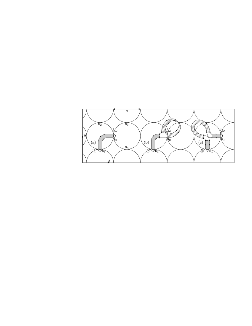
Figure 1: (a) Diagrams for the “bare” classical Hall conductivity $\sigma_{xy}^{(0)}$ [Eqs. (11) and (12)] of the granular metal. The contact ${\bf s}_{1}$ is connected to the contact $s_{0}$ by the intragrain diffuson (gray stripe). Same contributions from the contacts ${\bf s}_{2},{\bf s}_{3},{\bf s}_{4}$ have to be taken into account [Eq. (12)]. (b) Diagrams describing the weak localization correction to the conductance $G_{T}$ of the tunnel contact. A diagram with the Cooperon $\mathcal{C}_{0}$ (rendered with lines stripe) flipped down and the same two diagrams for the second contact also have to be considered. (c) An example of a diagram for the weak localization correction to the Hall resistance $R_{H}$ of the grain, which is expressed through the intragrain diffuson $D(\omega,{\bf r},{\bf r}^{\prime})$ [Eqs. (24) and (29)]. The diagram contributes to the renormalization of the diffusion coefficient $D_{0}$ [Eq. (24)], the complete set of such diagrams shown in Fig. 3. Weak localization corrections to the boundary condition (29) must be also taken into account (see Fig. 4).

The “bare” (i.e., without quantum effects) Hall conductivity of a granular metal is given byKEshort ; KElong

$$\sigma^{(0)}_{xy}=G_{T}^{2}R_{H}a^{2-d},$$ (11)

where $G_{T}$ is the conductance of the tunnel contact and $R_{H}$ is the Hall resistance of the grain. The latter is expressed through the intragrain diffuson as

$$R_{H}=\frac{1}{2e^{2}\nu}(\bar{D}_{\nearrow}-\bar{D}_{\searrow}+\bar{D}_{\swarrow}-\bar{D}_{\nwarrow}),$$ (12)

where

$$\bar{D}_{\alpha}=\frac{1}{S_{0}^{2}}\int d{\bf s}_{0}d{\bf s}_{a}\bar{D}({\bf s}_{0},{\bf s}_{a}),$$

with $a=1,2,3,4$ for $\alpha=\nearrow,\searrow,\swarrow,\nwarrow$, respectively [see Fig. 1(a)], $S_{0}$ is the area of the contact, and $\bar{D}({\bf r},{\bf r}^{\prime})$ is the diffusion propagator of a single grain at $\omega=0$ with discarded zero mode $1/(\omega\mathcal{V})$ ($\mathcal{V}$ is the grain volume). We specify $\bar{D}({\bf r},{\bf r}^{\prime})$ explicitly somewhat later. The essentially classical result (11) is given by the diagram in Fig. 1(a), in which the contacts ${\bf s}_{a}$, $a=1,2,3,4$, are connected to the contact ${\bf s}_{0}$ by the intragrain diffuson $\bar{D}({\bf r},{\bf r}^{\prime})$. In order not to overcomplicate the calculations we consider the range of frequencies $\omega\ll E_{\text{Th}}$ in this paper, which allows us to neglect the intragrain Coulomb interaction when calculating the bare Hall conductivity (see Ref. KElong, for details).

We emphasize the crucial for the Hall effect technical pointKEshort ; KElong : the nonvanishing contribution to the Hall conductivity [Eqs. (11) and (12)] comes from nonzero modes of the diffuson $\bar{D}({\bf r},{\bf r}^{\prime})$ only, whereas the zero mode $1/(\omega\mathcal{V})$ simply drops out due to the sign structure of Eq. (12).

Since the bare longitudinal conductivity equals

$$\sigma_{xx}^{(0)}=a^{2-d}G_{T},$$ (13)

the bare Hall resistivity, following from Eqs. (11) and (13),

$$\rho^{(0)}_{xy}=\frac{\sigma^{(0)}_{xy}}{\left(\sigma^{(0)}_{xx}\right)^{2}}=R_{H}a^{d-2}$$ (14)

is independent of the intergrain tunneling conductance $G_{T}$. It can be further shownKEshort ; KElong that the Hall resistance $R_{H}$ [Eq. (12)] is independent of the scattering time $\tau_{0}$ and Eq. (14) leads to Eq. (1).

In the first order in the inverse tunneling conductance $1/g_{T}$, the weak localization corrections to the classical result (11) are given by the sum of all “minimally crossed” diagrams. The “fan-shaped” ladder arising in such diagrams corresponds to the well-known particle-particle propagator called “Cooperon”, which can be formally defined for a granular metal in the same way as for an ordinary disordered metal:

$$\mathcal{C}(\omega,{\bf r}_{\bf i},{\bf r}_{\bf j}^{\prime})=\frac{1}{2\pi\nu}\langle\mathcal{G}(\varepsilon+\omega,{\bf r}_{\bf i},{\bf r}_{\bf j}^{\prime})\ \mathcal{G}(\varepsilon,{\bf r}_{\bf i},{\bf r}_{\bf j}^{\prime})\rangle_{U,t},\mbox{ }(\varepsilon+\omega)\varepsilon<0.$$ (15)

Here $\mathcal{G}$’s are the “exact” Green functions in the Matsubara technique and the average is taken over the intragrain and tunnel contact disorder with the help of Eqs. (5) and (7). The points ${\bf r}_{\bf i}$ and ${\bf r}_{\bf j}^{\prime}$ may belong to arbitrary distant grains ${\bf i}$ and ${\bf j}$.

One can calculate the Cooperon $\mathcal{C}(\omega,{\bf r}_{\bf i},{\bf r}_{\bf j}^{\prime})$ using the same diagrammatic rules as those for the diffusonKElong . They are governed by the condition $p_{F}a\gg 1$ ($p_{F}$ is the Fermi momentum in the grains) that each grain is a “good” metallic sample. This demands that the diagrammatic “paths” of the Green functions $\mathcal{G}(\varepsilon+\omega,{\bf r}_{\bf i},{\bf r}_{\bf j}^{\prime})$ and $\mathcal{G}(\varepsilon,{\bf r}_{\bf i},{\bf r}_{\bf j}^{\prime})$ through intermediate grains and contacts coincide. Therefore, the full Cooperon (15) is “composed” of the Cooperons

$$C(\omega,{\bf r},{\bf r}^{\prime})=\frac{1}{2\pi\nu}\langle\mathcal{G}(\varepsilon+\omega,{\bf r},{\bf r}^{\prime})\ \mathcal{G}(\varepsilon,{\bf r},{\bf r}^{\prime})\rangle_{U},\mbox{ }(\varepsilon+\omega)\varepsilon<0$$ (16)

of isolated grains. In Eq. (16), ${\bf r}$ and ${\bf r}^{\prime}$ belong to the same given grain and tunneling to the neighboring grains should be completely neglected.

Although in order to obtain nonvanishing Hall conductivity (11), one is forced to take nonzero modes in the intragrain diffuson $\bar{D}({\bf r},{\bf r}^{\prime})$ into accountKEshort ; KElong , the zero modes in the Cooperons themselves do not drop out from the expressions for WL corrections. Therefore due to the small size of the grains one may use the “zero-mode” approximation for the Cooperons, i.e., to leave only the zero mode $1/(\omega\mathcal{V})$ in each grain in the expression for the Cooperon (16). To do so, however, the condition (2) alone is not sufficient, since the Cooperons are sensitive to magnetic field, and in the presence of magnetic field an additional condition must be met. Namely, the magnetic flux $Ha^{2}$ threading through each grain must be smaller than the flux quantum $c/e$:

$$\frac{e}{c}Ha^{2}\ll 1.$$ (17)

Under the conditions (2) and (17) the spatial dependence of the intragrain Cooperon (16) coming from nonzero modes can be neglected and one gets:

$$C(\omega,{\bf r},{\bf r}^{\prime})\approx\frac{1}{\mathcal{V}}\frac{1}{\omega+{\cal E}(H)},$$

where ${\cal E}(H)\propto D_{0}(\frac{e}{c}Ha)^{2}$ is the “mass term” acquired due to dephasing by the magnetic field within the grain [$D_{0}$ is the intragrain diffusion coefficient defined after Eq. (24)]. After that, the Cooperon $\mathcal{C}(\omega,{\bf r}_{\bf i},{\bf r}_{\bf j}^{\prime})$ [Eq. (15)] of the whole granular system depends on the grain indices ${\bf i}$ and ${\bf j}$ only and we denote such “zero-mode” Cooperon as $\mathcal{C}_{0}(\omega,{\bf i},{\bf j})$. Its properties in the presence of magnetic field were studied in Refs. BCTV, ; BVG, . Since our main result, the vanishing WL correction to the Hall resistivity, does not depend on the explicit form of $\mathcal{C}_{0}(\omega,{\bf i},{\bf j})$, we do not repeat these properties here, reminding for reference only that in the absence of magnetic field and dephasing effects one has

$$\mathcal{C}_{0}(\omega,{\bf i},{\bf j})=\int\frac{a^{d}d^{d}{\bf q}}{(2\pi)^{d}}\frac{e^{ia{\bf q}({\bf i}-{\bf j})}}{\omega+2\Gamma\sum_{\beta}[1-\cos(q_{\beta}a)]},$$

where the integration is done over the first Brillouin zone ${\bf q}\in[-\pi/a,\pi/a]^{d}$ and $\beta=x,y$ in 2D and $\beta=x,y,z$ in 3D. Note, that we have removed the inverse grain volume $1/\mathcal{V}$ from the definition of $\mathcal{C}_{0}(\omega,{\bf i},{\bf j})$.

We can now proceed with calculations of the weak localization corrections. Conveniently, the contributions from the diagrams giving first-order corrections to HC $\sigma_{xy}^{(0)}$ are factorized according to the structure of Eq. (11), i.e., each diagram can be attributed to the renormalization of either the tunneling conductance $G_{T}$ of the contact or the Hall resistance $R_{H}$ of the grain. Below we study these two types of corrections separately.

III.1 Weak localization correction to $G_{T}$

First consider the diagram in Fig. 1(b). In this diagram the Cooperon $\mathcal{C}_{0}(\omega,{\bf i}+{\bf e}_{x},{\bf i})$ connects the points belonging to two sides (in the grains ${\bf i}+{\bf e}_{x}$ and ${\bf i}$) of the same contact $({\bf i}+{\bf e}_{x},{\bf i})$. Note that such diagrams arise form the “particle-particle pairing” $X_{{\bf i}+{\bf e}_{x},{\bf i}}(\tau)X_{{\bf i}+{\bf e}_{x},{\bf i}}(\tau_{1})$ [see Eqs. (6) and (10)] of the tunneling operators at the considered contact $({\bf i}+{\bf e}_{x},{\bf i})$, whereas in the diagram in Fig. 1(a) for the bare conductivity we have “particle-hole pairing” $X_{{\bf i}+{\bf e}_{x},{\bf i}}(\tau)X_{{\bf i},{\bf i}+{\bf e}_{x}}(\tau_{1})$.

Since the other elements of the diagram in Fig. 1(b) remain unaffected, this diagram can be attributed to the renormalization of the conductance $G_{T}$ of the tunnel contact in Eq. (11). Indeed, considering the same diagrams for the other contact in Fig. 1(a), for the relative correction to HC $\sigma_{xy}^{(0)}$ [Eq. (11)] we obtain:

$$\frac{\delta\sigma_{xy}^{(1)}(\omega)}{\sigma_{xy}^{(0)}}=2\frac{\delta G_{T}(\omega)}{G_{T}},$$ (18)

where

$$\frac{\delta G_{T}(\omega)}{G_{T}}=\frac{1}{2\pi\nu\mathcal{V}}[\mathcal{C}_{0}(\omega,{\bf i}+{\bf a},{\bf i})+\mathcal{C}_{0}(\omega,{\bf i},{\bf i}+{\bf a})],$$ (19)

and ${\bf a}={\bf e}_{x}$ or ${\bf a}={\bf e}_{y}$, [assuming the square/cubic symmetry of the lattice, we do not distinguish between $x$ and $y$ directions]. In Eq. (18), the factor $2$ stands for two contacts according to the square $G_{T}^{2}$ in Eq. (11). As expected, the expression (19) for the relative correction to $G_{T}$ obtained from the diagrams in Fig. 1(b) coincides with the one obtained from calculating WL correction to the longitudinal conductivity $\sigma_{xx}^{(0)}$ in Refs. BelUD, ; BCTV, ; BVG, :

$$\frac{\delta\sigma_{xx}^{WL}(\omega)}{\sigma_{xx}^{(0)}}=\frac{\delta G_{T}(\omega)}{G_{T}}.$$ (20)

Since the correction (18) contributes solely to the renormalization of the tunneling conductance $G_{T}$ and the bare HR $\rho_{xy}^{(0)}$ [Eq. (14)] simply does not contain $G_{T}$, the corresponding WL correction to HR from the diagrams in Fig. 1(b) vanishes:

$$\frac{\delta\rho_{xy}^{(1)}(\omega)}{\rho_{xy}^{(0)}}=\frac{\delta\sigma_{xy}^{(1)}(\omega)}{\sigma_{xy}^{(0)}}-2\frac{\delta\sigma_{xx}^{WL}(\omega)}{\sigma_{xx}^{(0)}}\equiv 0.$$ (21)

III.2 Weak localization correction to $R_{H}$

Now let us consider the diagram shown in Fig. 1(c). This diagram describes the effect of localization on the intragrain diffuson $D(\omega,{\bf r},{\bf r}^{\prime})$ and, eventually, contributes to the renormalization of the Hall resistance $R_{H}$ of the grain, expressed through the diffuson according to Eq. (12). The aim of this section is to show that the WL correction to the Hall resistance (12) arising from all such diagrams actually vanishes:

$$\delta R_{H}^{WL}=0.$$ (22)

We remind the reader that the intragrain diffuson is defined formally as

$$D(\omega,{\bf r},{\bf r}^{\prime})\equiv\frac{1}{2\pi\nu}\langle\mathcal{G}(\varepsilon+\omega,{\bf r},{\bf r}^{\prime})\mathcal{G}(\varepsilon,{\bf r}^{\prime},{\bf r})\rangle_{U},\mbox{ }(\varepsilon+\omega)\varepsilon<0.$$ (23)

where $\langle\ldots\rangle_{U}$ denotes the averaging over the intragrain disorder according to Eq. (5).

III.2.1 Intragrain diffuson in the absence of weak localization effects

In the absence of weak localization effects (i.e., in the “noncrossing approximation”AGD ) the average (23) is given by a series of ladder-type diagrams. The summation of this series is equivalent to solving a certain integral equation, which in the diffusive limit ($\omega\tau_{0}\ll 1$ and $l\ll a$) can be reduced to a differential diffusion equation

$$(\omega-D_{0}\nabla_{\bf r}^{2})D(\omega,{\bf r},{\bf r}^{\prime})=\delta({\bf r}-{\bf r}^{\prime}).$$ (24)

Here $D_{0}=v_{F}l/3$ is the classical diffusion coefficient in the grain ($v_{F}$ is the Fermi velocity, $l=v_{F}\tau_{0}$ is the electron mean free path, $D_{0}$ is not affected by magnetic field, such that $\omega_{H}\tau_{0}\ll 1$).

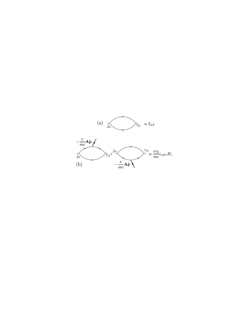
Figure 2: Diagrams for the current-coordinate correlation function $\langle j_{\alpha}r_{\beta}\rangle_{0}$ [Eqs. (26) and (28)] in the absence of weak localization. Fermionic lines denote the Green function $[G(\varepsilon,{\bf p})]^{-1}=i\varepsilon-\xi_{\bf p}+\frac{i}{2\tau_{0}}\text{sgn}\,\varepsilon$ of a bulk metal with $H=0$. (a) Magnetic-field-independent part of $\langle j_{\alpha}r_{\beta}\rangle_{0}$ giving the LHS of the boundary condition (29). (b) Linear in magnetic field part of $\langle j_{\alpha}r_{\beta}\rangle_{0}$ obtained by inserting the “magnetic vertex” $-\frac{e}{mc}{\bf A}\hat{{\bf p}}$ in all possible ways into the diagram (a) and giving the RHS of Eq. (29).

For a finite system (a grain), Eq. (24) must be supplied by a proper boundary condition. In Ref. KElong, we have shown that the boundary condition in the diffusive case has the form

$$n_{\alpha}\langle j_{\alpha}r_{\beta}\rangle_{0}\nabla_{{\bf r}\beta}D(\omega,{\bf r},{\bf r}^{\prime})|_{{\bf r}\in S}=0.$$ (25)

Here, the coordinate ${\bf r}$ belongs to the grain boundary $S$, the unit vector ${\bf n}$ normal to the grain boundary points outside the grain, $\alpha,\beta=x,y,z$, and

$$\langle j_{\alpha}r_{\beta}\rangle_{0}=\int d{\bf x}\hat{j}_{{\bf r}\alpha}[G(\varepsilon+\omega,{\bf r},{\bf x})G(\varepsilon,{\bf x},{\bf r})]({\bf x}-{\bf r})_{\beta}$$ (26)

is the current-coordinate correlation function. In Eq. (26), $G(\varepsilon+\omega,{\bf r},{\bf x})=\langle\mathcal{G}(\varepsilon+\omega,{\bf r},{\bf x})\rangle_{U}$ is the disorder-averaged Green function of the grain and the current operator ${\bf j}_{\bf r}$ acts on the product of two Green functions as

$$\hat{{\bf j}}_{\bf r}[G(\varepsilon+\omega,{\bf r},{\bf x})G(\varepsilon,{\bf x},{\bf r})]=$$

$$=\frac{1}{2m}[G(\varepsilon,{\bf x},{\bf r})(-i\nabla_{\bf r})G(\varepsilon+\omega,{\bf r},{\bf x})$$

$$+G(\varepsilon+\omega,{\bf r},{\bf x})(i\nabla_{\bf r})G(\varepsilon,{\bf x},{\bf r})]$$

$$-\frac{e}{mc}{\bf A}({\bf r})G(\varepsilon+\omega,{\bf r},{\bf x})\mathcal{G}(\varepsilon,{\bf x},{\bf r}),$$ (27)

where the vector potential ${\bf A}({\bf r})$ corresponds to the magnetic field $H$.

Owing to the small spatial scale ($\sim l\ll a$) of the kernel in Eq. (26), $\langle j_{\alpha}r_{\beta}\rangle_{0}$ may be evaluated for ${\bf r}$ located not directly on the grain boundary, but a few $l$ away from it in the bulk of the grain, where the expressions for the bulk can be used for $G$’s. Note that the ladder contribution to $\langle j_{\alpha}r_{\beta}\rangle_{0}$ vanishes in the case of the white noise-disorder [Eq. (5)].

As we are study Hall transport, the correlation function $\langle j_{\alpha}r_{\beta}\rangle_{0}$ has to be calculated taking the magnetic field $H$ into account, which may be done in the linear in $H$ order, since the condition $\omega_{H}\tau_{0}\ll 1$ is assumed to be met. The calculations can be performed with the help of the diagrammatic technique either by directly expanding Green functions $G$ in the vector potential ${\bf A}({\bf r})$ or using an explicitly gauge-invariant approach developed by Khodas and Finkel’stein in Ref. Khodas, . We choose the former approach here. The diagrams for $\langle j_{\alpha}r_{\beta}\rangle_{0}$ in the absence of WL effects are given in Fig. 2 and we obtainKElong :

$$\langle j_{\alpha}r_{\beta}\rangle_{0}=\Lambda\left(\delta_{\alpha\beta}+\frac{e\tau_{0}}{mc}\epsilon_{\alpha\beta\gamma}H_{\gamma}\right),$$ (28)

where $\epsilon_{\alpha\beta\gamma}$ is the totally antisymmetric tensor, $\epsilon_{xyz}=1$, and $\Lambda=-(2\pi/3)\nu l^{2}$ is an irrelevant for the boundary condition (25) prefactor. Inserting Eq. (28) into Eq. (25), we get

$$({\bf n},\nabla_{\bf r}D)|_{{\bf r}\in S}=\omega_{H}\tau_{0}({\bf t},\nabla_{\bf r}D)|_{{\bf r}\in S},$$ (29)

where ${\bf t}=[{\bf n},{\bf H}]/H$ is the tangent vector pointing in the direction opposite to the edge drift.

The propagator $\bar{D}({\bf r},{\bf r}^{\prime})$ entering the expression (12) for the Hall resistance $R_{H}$ of the grain, satisfies Eqs. (24) and (29) with $\omega=0$, i.e., $\bar{D}({\bf r},{\bf r}^{\prime})$ is a Green function for the Poisson equation with the boundary condition (29).

III.2.2 Intragrain diffuson renormalized by weak localization effects

We can now proceed with WL corrections to the intragrain diffuson $D(\omega,{\bf r},{\bf r}^{\prime})$. Since neglecting localization effects the diffuson $D(\omega,{\bf r},{\bf r}^{\prime})$ [Eq. (23)] has been reduced to the solution of Eqs. (24) and (25), our task now is to find out how these equations are affected by weak localization. It is very important that for a finite system with boundary (grain) one has to renormalize not only the diffusion equation (24) itself, but also the boundary condition (25) for the diffuson.

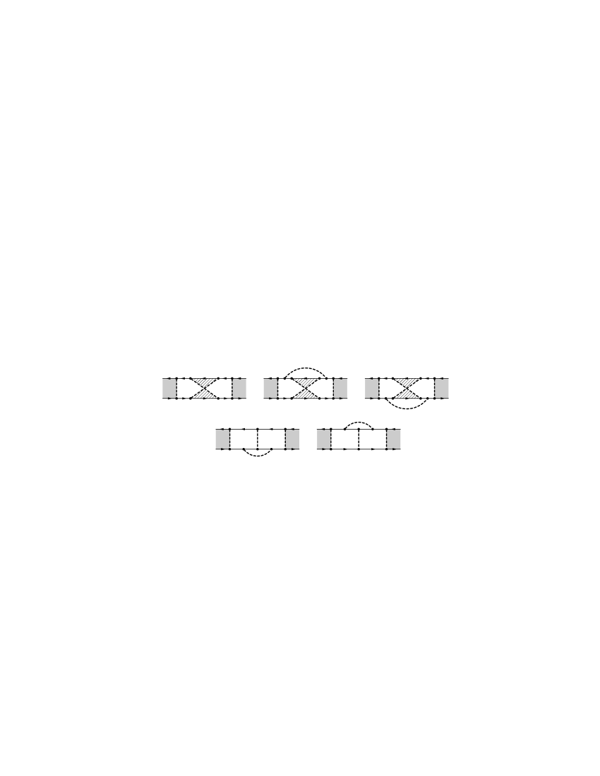
Figure 3: Diagrams for the weak localization correction to the diffusion coefficient $D_{0}$ [Eqs. (30) and (31)] of the intragrain diffuson $D(\omega,{\bf r},{\bf r}^{\prime})$ (gray blocks). Diagrams in the upper row form a Hikami box, the twisted rendered with lines block denotes the Cooperon $\mathcal{C}_{0}(\omega,{\bf i},{\bf i})$. Diagrams in the lower row are of the same order as the sum of those in the upper row and are missing in the ladder summation for $\mathcal{C}_{0}(\omega,{\bf i},{\bf i})$.

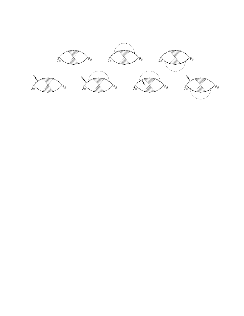
Figure 4: Diagrams for the weak localization corrections [Eq. (32)] to the current-coordinate correlation function $\langle j_{\alpha}r_{\beta}\rangle_{0}$ [Eqs. (26) and (28)]. Diagrams in the upper row forming a Hikami box describe the correction to the magnetic-field-independent part of $\langle j_{\alpha}r_{\beta}\rangle_{0}$ [Fig. 2(a)]. Diagrams in the lower row describe the correction to the linear in the magnetic field part of $\langle j_{\alpha}r_{\beta}\rangle_{0}$ [Fig. 2(b)]. Similar insertions of the magnetic vertex into the right block of Green functions and the upside-down flip of such diagrams must also be considered.

We start by considering the diffusion equation (24). In a bulk metal effects of localization on the diffusive electron motion were first studied in Ref. GLK, by Gorkov, Larkin, and Khmelnitski. It was shown that the diffusion equation (24) remains valid, but the diffusion constant $D_{0}$ is renormalized. The diagrams describing renormalization of $D_{0}$ are obtained by inserting the “fan-shaped” ladder into the ordinary ladder describing the diffuson $D(\omega,{\bf r},{\bf r}^{\prime})$, as shown in Fig. 3. Their calculation is more challenging for a granular system due to the possibility of tunneling between the grains. Nevertheless, under the assumed conditions (2) and (17) we obtain a result essentially the same as that of Ref. GLK, for the renormalized diffusion coefficient:

$$\tilde{D}_{0}(\omega)=D_{0}[1-c(\omega)],$$ (30)

where

$$c(\omega)=\frac{1}{\pi\nu\mathcal{V}}\mathcal{C}_{0}(\omega,{\bf i},{\bf i})$$ (31)

is given by the zero-mode Cooperon with coinciding points. Since the characteristic scale of the Cooperon is $\mathcal{C}_{0}(\omega,{\bf i},{\bf i})\sim 1/\Gamma$ and the mean level spacing in each grain is $\delta=1/(\nu\mathcal{V})$, the relative correction $c(\omega)\sim\delta/\Gamma=1/g_{T}$ is proportional to the inverse intergrain conductance $1/g_{T}$.

More interestingly, for a finite system one also has to consider the effect of WL on the boundary condition (25). The sensitivity of the boundary condition to WL effects is crucial for the Hall transport, since, as it was discussed in Ref. KElong, , the differences $\bar{D}_{\nearrow}-\bar{D}_{\searrow}$ and $\bar{D}_{\swarrow}-\bar{D}_{\nwarrow}$ in Eq. (12) for $R_{H}$ are nonvanishing solely due to the presence of the magnetic field in Eq. (25). Since the boundary condition (25) is determined by the correlation function (26), we need to find WL correction to this quantity. The corresponding diagrams are shown in Fig. 4. Their calculation is somewhat cumbersome, but straightforward, and yields the following result for the renormalized correlation function:

$$\langle j_{\alpha}r_{\beta}\rangle=\Lambda\left\{\delta_{\alpha\beta}[1-c(\omega)]+\frac{e\tau_{0}}{mc}\epsilon_{\alpha\beta\gamma}H_{\gamma}[1-2c(\omega)]\right\},$$ (32)

where $c(\omega)$ is given by Eq. (31).

As a result, replacing $D_{0}$ by $\tilde{D}_{0}(\omega)$ [Eq. (30)] in Eq. (24) and $\langle j_{\alpha}r_{\beta}\rangle_{0}$ by $\langle j_{\alpha}r_{\beta}\rangle$ [Eq. (32)] in Eq. (25), we obtain that the renormalized diffuson satisfies the equation

$$\left\{\omega-D_{0}[1-c(\omega)]\nabla_{\bf r}^{2}\right\}D(\omega,{\bf r},{\bf r}^{\prime})=\delta({\bf r}-{\bf r}^{\prime})$$ (33)

and the boundary condition

$$({\bf n},\nabla_{\bf r}D)|_{{\bf r}\in S}=\omega_{H}\tau_{0}[1-c(\omega)]({\bf t},\nabla_{\bf r}D)|_{{\bf r}\in S}.$$ (34)

instead of Eqs. (24) and (29), respectively. In Eq. (34) we put $[1-2c(\omega)]/[1-c(\omega)]\approx 1-c(\omega)$, since $c(\omega)\ll 1$ within the validity of the perturbation approach.

III.2.3 Vanishing weak localization correction to the grain Hall resistance $R_{H}$

Now let us see how the obtained renormalizations affect the Hall resistance $R_{H}$ [Eq. (12)] of the grain. Although Eqs. (33) and (34) cannot be solved for an arbitrary shape of the grains, this is not actually necessary and the needed conclusions about $R_{H}$ can be drawn based on the following rather simple analysis.

The characteristic value of $\bar{D}_{\alpha}$’s in Eq. (12) can be estimated from Eq. (33) as

$$\bar{D}_{\alpha}\propto\frac{1}{a^{3}}\frac{1}{D_{0}[1-c(\omega)]/a^{2}}.$$ (35)

The differences $\bar{D}_{\nearrow}-\bar{D}_{\searrow}=\bar{D}_{\swarrow}-\bar{D}_{\nwarrow}$ in Eq. (12), however, require a more accurate estimate, since they are nonzero only in the presence of magnetic field $H\neq 0$ due to the directional asymmetry $\bar{D}({\bf r},{\bf r}^{\prime})\neq\bar{D}({\bf r}^{\prime},{\bf r})$, and vanish for $H=0$, when $\bar{D}({\bf r},{\bf r}^{\prime})=\bar{D}({\bf r}^{\prime},{\bf r})$. The effect of magnetic field is contained in the right-hand side (RHS) of the boundary condition (34). Since the difference $\bar{D}_{\nearrow}-\bar{D}_{\searrow}$ is linear in $H$ for $\omega_{H}\tau_{0}\ll 1$, it is linear in the factor $\omega_{H}\tau_{0}[1-c(\omega)]$ in the RHS of Eq. (34). Combining this fact with Eq. (35), we obtain

$$\bar{D}_{\nearrow}-\bar{D}_{\searrow}\propto\frac{1}{a^{3}}\frac{\omega_{H}\tau_{0}[1-c(\omega)]}{D_{0}[1-c(\omega)]/a^{2}}=\frac{1}{a^{3}}\frac{\omega_{H}\tau_{0}}{D_{0}/a^{2}},$$ (36)

where the proportionality coefficient depends on the grain geometry only. We see that the factors $[1-c(\omega)]$ in the numerator and denominator arising from the boundary condition (34) and differential equation (33), respectively, cancel each other. Therefore, the Hall resistance $R_{H}$ [Eq. (12)] of the grain remains unaffected by weak localization effects and the correction $\delta R_{H}^{WL}$ to it vanishes [Eq. (22)]. Consequently, the corresponding contributions to the Hall conductivity and resistivity vanish:

$$\frac{\delta\rho_{xy}^{(2)}(\omega)}{\rho_{xy}^{(0)}}=\frac{\delta\sigma_{xy}^{(2)}(\omega)}{\sigma_{xy}^{(0)}}=\frac{\delta R_{H}^{WL}}{R_{H}}\equiv 0.$$ (37)

IV Results and conclusion

Combining Eqs. (21) and (37), we obtain that the first-order in the inverse tunneling conductance $1/g_{T}$ weak localization correction $\delta\rho_{xy}^{WL}=\delta\rho_{xy}^{(1)}+\delta\rho_{xy}^{(2)}$ to the Hall resistivity of a granular metal vanishes identically:

$$\delta\rho_{xy}^{WL}=0.$$ (38)

The weak localization correction $\delta\sigma_{xy}^{WL}=\delta\sigma_{xy}^{(1)}+\delta\sigma_{xy}^{(2)}=\delta\sigma_{xy}^{(1)}$ [Eqs. (18), (20), and (37)] to the Hall conductivity originates from the renormalization of the tunneling conductance $G_{T}$ only, the corresponding relative correction being twice as large as that to the longitudinal conductivity:

$$\frac{\delta\sigma_{xy}^{WL}}{\sigma_{xy}^{(0)}}=2\frac{\delta\sigma_{xx}^{WL}}{\sigma_{xx}^{(0)}}.$$

The WL correction $\delta\sigma_{xx}^{WL}$ was studied in Refs. BelUD, ; BCTV, ; BVG, .

Whether the exact cancellation (38) obtained in the first order in $1/g_{T}$ is violated in higher orders or not remains a question of a separate investigation. What is important, however, is that in the same first order in $1/g_{T}$ (i) logarithmic temperature-dependent corrections to both the longitudinal $\rho_{xx}$ET ; BELV and Hall $\rho_{xy}$KEshort ; KElong resistivities due to Coulomb interactions exist; (ii) weak localization correction $\delta\rho_{xx}^{WL}(H)$ to $\rho_{xx}$ existsBelUD ; BCTV ; BVG , being sensitive to the magnetic fieldBCTV ; BVG . Therefore, we come to the conclusion that in the leading order in $1/g_{T}$, in which quantum effects do come into play, the effect of weak localization on the Hall resistivity is absent [Eq. (38)].

Experimentally, our result (38) may be tested by measuring the dependence of the Hall coefficient $\rho_{xy}(H)/H$ on magnetic field $H$. Since the weak localization correction $\delta\rho_{xx}^{WL}(H)$ is sensitive to the magnetic field, Eq. (38) states that in the range of sufficiently low magnetic fields $H$, in which the relative change in the longitudinal resistivity $\rho_{xx}(H)$ of the order of $1/g_{T}$ due to localization effects is predictedBCTV ; BVG , no comparable change in $\rho_{xy}(H)/H$ is expected.

In conclusion, we have studied the effects of weak localization on Hall transport in granular metals. Calculating the first-order in the inverse intergrain conductance corrections, we found that the Hall resistivity of the system remains unaffected by weak localization effects. This result is in agreement with the one obtained for ordinary disordered metals. It holds for arbitrary relevant values of temperatures $T$ and magnetic fields $H$, both in the universal “homogeneous” regime of very low $T$ and $H$ and in the “structure-dependent” regime of higher $T$ or $H$.

We thank Igor S. Beloborodov, Yuli V. Nazarov, and Anatoly F. Volkov for illuminating discussions and acknowledge financial support of Degussa AG (Germany), SFB Transregio 12, the state of North-Rhine Westfalia, and the European Union.

References

• (1) I. S. Beloborodov, A. V. Lopatin, V. M. Vinokur, and K. B. Efetov, Rev. Mod. Phys. 79, 469 (2007).
• (2) M. Yu. Kharitonov, K. B. Efetov, arXiv:cond-mat/0609736 [Phys. Rev. Lett. (to be published)].
• (3) M. Yu. Kharitonov, K. B. Efetov, arXiv:0706.3866.
• (4) I.S. Beloborodov, A.V. Lopatin, and V.M. Vinokur, Phys. Rev.B 70, 205120 (2004).
• (5) C. Biagini, T. Caneva, V. Tognetti, and A.A. Varlamov, Phys. Rev. B 72, 041102(R) (2005).
• (6) Ya.M. Blanter, V.M. Vinokur, and L.I. Glazman, Phys. Rev. B 73, 165322 (2006).
• (7) H. Fukuyama, J. Phys. Soc. Japan 49, 644 (1980).
• (8) B.L. Altshuler, D.E. Khmelnitski, A.I. Larkin, and P.A. Lee, Phys. Rev. B 22, 5142 (1980).
• (9) A.A. Abrikosov, L.P. Gorkov, and I.E. Dzyaloshinski, Methods of Quantum Field Theory in Statistical Physics (Prentice-Hall, Englewood Cliffs, New Jersey, 1963).
• (10) M. Khodas, A. M. Finkel’stein, Phys. Rev. B 68, 155114 (2003).
• (11) L. Gorkov, A. Larkin and D. Khmelnitski, Pis’ma Zh. Eksp. Teor. Fiz. 30, 248 (1979) [Sov. Phys JETP Lett. 30, 228 (1979)].
• (12) K. B. Efetov and A. Tschersich, Europhys. Lett. 59, 114, (2002); Phys. Rev. B 67, 174205, (2003).
• (13) I. S. Beloborodov, K. B. Efetov, A. V. Lopatin, and V. M. Vinokur, Phys. Rev. Lett 91, 246801, (2003).