On the Complexity of the Interlace Polynomial

Abstract

We consider the two-variable interlace polynomial introduced by Arratia, Bollobás and Sorkin (2004). We develop graph transformations which allow us to derive point-to-point reductions for the interlace polynomial. Exploiting these reductions we obtain new results concerning the computational complexity of evaluating the interlace polynomial at a fixed point. Regarding exact evaluation, we prove that the interlace polynomial is $\mathsf{\#P}$-hard to evaluate at every point of the plane, except on one line, where it is trivially polynomial time computable, and four lines, where the complexity is still open. This solves a problem posed by Arratia, Bollobás and Sorkin (2004). In particular, three specializations of the two-variable interlace polynomial, the vertex-nullity interlace polynomial, the vertex-rank interlace polynomial and the independent set polynomial, are almost everywhere $\mathsf{\#P}$-hard to evaluate, too. For the independent set polynomial, our reductions allow us to prove that it is even hard to approximate at every point except at $0$.

1 Introduction

The number of Euler circuits in specific graphs and their interlacings turned out to be a central issue in the solution of a problem related to DNA sequencing by hybridization [ABCS00]. This led to the definition of a new graph polynomial, the one-variable interlace polynomial [ABS04a]. Further research on this polynomial inspired the definition of a two-variable interlace polynomial $q(G;x,y)$ containing as special cases the following graph polynomials: $q_{N}(G;y)=q(G;2,y)$ is the original one-variable interlace polynomial which was renamed to “vertex-nullity interlace polynomial”, $q_{R}(G;x)=q(G;x,2)$ is the new “vertex-rank interlace polynomial” and $I(G;x)=q(G;1,1+x)$ is the independent set polynomial [ABS04b].

Although the interlace polynomial $q(G;x,y)$ is a different object from the celebrated Tutte polynomial (also known as dichromatic polynomial, see, for instance, [Tut84]), they are also similar to each other. While the Tutte polynomial can be defined recursively by a deletion-contraction identity on edges, the interlace polynomial satisfies recurrence relations involving several operations on vertices (deletion, pivotization, complementation).

Besides the deletion-contraction identity, the so called state expansion is a well-known way to define the Tutte polynomial. Here the similarity to the two-variable interlace polynomial is especially striking: while the interlace polynomial is defined as a sum over all vertex subsets of the graph using the rank of adjacency matrices (see (2.1)), the state expansion of the Tutte polynomial can be interpreted as a sum over all edge subsets of the graph using the rank of incidence matrices (see (4.1)) [ABS04b, Section 1].

References to further work on the interlace polynomial can be found in [ABS04b] and [EMS07].

1.1 Previous work

The aim of this paper is to explore the computational complexity of evaluating the two-variable interlace polynomial $q(G;x,y)$. For the Tutte polynomial this problem was solved in [JVW90]: Evaluating the Tutte polynomial is $\mathsf{\#P}$-hard at any algebraical point of the plane, except on the hyperbola $(x-1)(y-1)=1$ and at a few special points, where the Tutte polynomial can be evaluated in polynomial time. For the two-variable interlace polynomial $q(G;x,y)$, only on a one-dimensional subset of the plane (on the lines $x=2$ and $x=1$) some results about the evaluation complexity are known.

A connection between the vertex-nullity interlace polynomial and the Tutte polynomial of planar graphs [ABS04a, End of Section 7], [EMS07, Theorem 3.1] shows that evaluating $q$ is $\mathsf{\#P}$-hard almost everywhere on the line $x=2$ (Corollary 4.4).

It has also been noticed that $q(G;1,2)$ evaluates to the number of independent sets of $G$ [ABS04b, Section 5], which is $\mathsf{\#P}$-hard to compute [Val79]. Recent work on the matching generating polynomial [AM07] implies that evaluating $q$ is $\mathsf{\#P}$-hard almost everywhere on the line $x=1$ (Corollary 4.10).

A key ingredient of [JVW90] is to apply graph transformations known as stretching and thickening of edges. For the Tutte polynomial, these graph transformations allow us to reduce the evaluation at one point to the evaluation at another point. For the interlace polynomial no such graph transformations have been given so far.

1.2 Our results

We develop three graph transformations which are useful for the interlace polynomial: cloning of vertices and adding combs or cycles to the vertices. Applying these transformations allows us to reduce the evaluation of the interlace polynomial at some point to the evaluation of it at another point, see Theorem 3.3, Theorem 3.5 and Theorem 3.7. We exploit this to obtain the following new results about the computational complexity of $q(G;x,y)$.

We prove that the two-variable interlace polynomial $q(G;x,y)$ is $\mathsf{\#P}$-hard to evaluate at almost every point of the plane, Theorem 4.11, see also Figure 1. Even though there are some unknown (gray, in Figure 1) lines left on the complexity map for $q$, this solves a challenge posed in [ABS04b, Section 5]. In particular we obtain the new result that evaluating the vertex-rank interlace polynomial $q_{R}(G;x)$ is $\mathsf{\#P}$-hard at almost every point (Corollary 4.12). Our techniques also give a new proof that the independent set polynomial is $\mathsf{\#P}$-hard to evaluate almost everywhere (Corollary 4.10).

Apart from these results on the computational complexity of evaluating the interlace polynomial exactly, we also show that the values of the independent set polynomial (which is the interlace polynomial $q(G;x,y)$ on the line $x=1$) are hard to approximate almost everywhere (Theorem 5.4).

2 Preliminaries

2.1 Interlace Polynomials

We consider undirected graphs without multiple edges but with self loops allowed. Let $G=(V,E)$ be such a graph and $A\subseteq V$. By $G[A]$ we denote $(A,\{e|e\in E,e\subseteq A\})$, the subgraph of $G$ induced by $A$. The adjacency matrix of $G$ is the symmetric $n\times n$-matrix $M=(m_{ij})$ over $\mathbb{F}_{2}=\{0,1\}$ with $m_{i,j}=1$ iff $\{i,j\}\in E$. The rank of this matrix is its rank over $\mathbb{F}_{2}$. Slightly abusing notation we write $rk(G)$ for this rank. This allows us to define the two-variable interlace polynomial.

Definition 2.1 ([ABS04b]).

Let $G=(V,E)$ be an undirected graph. The interlace polynomial $q(G;x,y)$ of $G$ is defined as

$$q(G;x,y)=\sum_{A\subseteq V}(x-1)^{rk(G[A])}(y-1)^{|A|-rk(G[A])}.$$ (2.1)

In Section 3 we will introduce graph transformations which perform one and the same operation (cloning one single vertex, adding a comb or a cycle to one single vertex, resp.) on every vertex of a graph. Instead of relating the interlace polynomial of the original graph directly to the interlace polynomial of the transformed graph, we will analyze how, say, cloning one single vertex changes the interlace polynomial. To express this, we must be able to treat the vertex being cloned in a particular way, differently from the other vertices. This becomes possible using a multivariate version of the interlace polynomial, in which each vertex has its own variable. Once we can express the effect of cloning one vertex by an appropriate substitution of the vertex variable in the multivariate interlace polynomial, cloning all the vertices amounts to a simple substitution of all vertex variables and brings us back to a bivariate interlace polynomial. This procedure has been applied successfully to the Tutte polynomial [Sok05, BM06].

We choose the following multivariate interlace polynomial, which is similar to the multivariate Tutte polynomial of Sokal [Sok05] and a specialization of the multivariate interlace polynomial defined by Courcelle [Cou07].

Definition 2.2.

Let $G=(V,E)$ be an undirected graph. For each $v\in V$ let $x_{v}$ be an indeterminate. Writing $x_{A}$ for $\prod_{v\in A}x_{v}$, we define the following multivariate interlace polynomial:

$$P(G;u,\mathbf{x})=\sum_{A\subseteq V}x_{A}u^{rk(G[A])}.$$

Substituting each $x_{v}$ in $P(G;u,\mathbf{x})$ by $x$, we obtain another bivariate interlace polynomial:

$$P(G;u,x)=\sum_{A\subseteq V}x^{|A|}u^{rk(G[A])}.$$

An easy calculation proves that $q$ and $P$ are closely related:

Lemma 2.3.

Let $G$ be a graph. Then we have the polynomial identities $q(G;x,y)=P(G;\frac{x-1}{y-1},y-1)$ and $P(G;u,x)=q(G;ux+1,x+1)$. ∎

2.2 Evaluating Graph Polynomials

Given $\xi,\upsilon\in\mathbb{Q}$ we want to analyze the following computational problem:

Input

Graph $G$

Output

$q(G;\xi,\upsilon)$

This is what we mean by “evaluating the interlace polynomial $q$ at the point $(\xi,\upsilon)$”. As an abbreviation for this computational problem we write

$$q(\xi,\upsilon),$$

which should not be confused with the expression $q(G;\xi,\upsilon)$ denoting just a value in $\mathbb{Q}$. Evaluating other graph polynomials such as $P$, $q_{N}$, $q_{R}$ and $I$ is defined accordingly.

If $P_{1}$ and $P_{2}$ are computational problems we use $P_{1}\preceq_{T}P_{2}$ ($P_{1}\preceq^{\mathtt{m}}P_{2}$) to denote a polynomial time Turing reduction (polynomial time many-one reduction, resp.) from $P_{1}$ to $P_{2}$. For instance, Lemma 2.3 gives

Corollary 2.4.

For $\xi,\upsilon\in\tilde{\mathbb{Q}}$, $\upsilon\neq 1$, we have $q(\xi,\upsilon)\preceq^{\mathtt{m}}P(\frac{\xi-1}{\upsilon-1},\upsilon-1)$. For $\mu,\xi\in\tilde{\mathbb{Q}}$ we have $P(\mu,\xi)\preceq^{\mathtt{m}}q(\mu\xi+1,\xi+1)$. ∎

Here $\tilde{\mathbb{Q}}$ denotes some finite dimensional field extension $\mathbb{Q}\subseteq\tilde{\mathbb{Q}}\subseteq\mathbb{R}$, which has a discrete representation. As $\sqrt{2}$ will play an important role but we are not able to use arbitrary real numbers as the input for a Turing machine, we use $\tilde{\mathbb{Q}}$ instead of $\mathbb{Q}$ or $\mathbb{R}$. We fix some $\tilde{\mathbb{Q}}$ for the rest of this paper. This construction is done in the spirit of Jaeger, Vertigan, and Welsh [JVW90] who also propose to adjoin a finite number of points to $\mathbb{Q}$ in order to talk about the complexity at irrational points. To some extent, this is an ad hoc construction, but it is sufficient for this work.

3 Graph Transformations for the Interlace Polynomial

Now we describe our graph transformations, vertex cloning and adding combs or cycles to the vertices. The main results of this section are Theorem 3.3, Theorem 3.5 and Theorem 3.7, which describe the effect of these graph transformations on the interlace polynomial.

3.1 Cloning

Cloning vertices in the graph yields our first graph transformation.

Cloning one vertex

Let $G=(V,E)$ be a graph. Let $a\in V$ be some vertex (the one which will be cloned) and $N$ the set of neighbors of $a$, $V^{\prime}=V\setminus\{a\}$ and $M=V^{\prime}\setminus N$. The graph $G$ with $a$ cloned, $G_{aa}$, is obtained out of $G$ in the following way: Insert a new isolated vertex $a^{\prime}$. Connect $a^{\prime}$ to all vertices in $N$. If $a$ does not have a self loop, we are done. Otherwise connect $a$ and $a^{\prime}$ and insert a self loop at $a^{\prime}$. Thus, adjacency matrices of the original (cloned, resp.) graph are

$$B=\begin{array}[]{c|ccc}&a&N&M\\ \hline\cr a&b&\mathbf{1}&\mathbf{0}\\ N&\mathbf{1}&A_{11}&A_{12}\\ M&\mathbf{0}&A_{21}&A_{22}\end{array}\quad\quad\text{and}\quad\quad B_{aa}=\begin{array}[]{c|cccc}&a^{\prime}&a&N&M\\ \hline\cr a^{\prime}&b&b&\mathbf{1}&\mathbf{0}\\ a&b&b&\mathbf{1}&\mathbf{0}\\ N&\mathbf{1}&\mathbf{1}&A_{11}&A_{12}\\ M&\mathbf{0}&\mathbf{0}&A_{21}&A_{22}\end{array}\quad,\quad\text{resp,}$$ (3.1)

where $b=1$ if $a$ has a self loop and $b=0$ otherwise. As the first column of $B_{aa}$ equals its second column, as well as the first row equals the second row, we can remove the first row and the first column of $B_{aa}$ without changing the rank. This also holds when we consider the adjacency matrices of $G[A]$ ($G_{aa}[A]$, resp.) instead of $G$ ($G_{aa}$ resp.) for $A\subseteq V^{\prime}$. Thus we have for any $A\subseteq V^{\prime}$

$$rk(G_{aa}[A]) =rk(G[A]),$$ (3.2)

$$rk(G_{aa}[A\cup\{a,a^{\prime}\}]) =rk(G_{aa}[A\cup\{a\}])=rk(G_{aa}[A\cup\{a^{\prime}\}])=rk(G[A\cup\{a\}]).$$ (3.3)

Let $\mathbf{x}=(x_{v})_{v\in V(G_{aa})}$ be a labeling of the vertices of $G_{aa}$ by indeterminates. Define $\mathbf{X}$ to denote the following labeling of the vertices of $G$: $X_{v}:=x_{v}$ for all $v\in V^{\prime}$, $X_{a}:=(1+x_{a})(1+x_{a^{\prime}})-1=x_{a}+x_{a^{\prime}}+x_{a}x_{a^{\prime}}$. Then we have

Lemma 3.1.

$P(G_{aa};u,\mathbf{x})=P(G;u,\mathbf{X})$.

Proof.

On the one hand we have

$$P(G_{aa};u,\mathbf{x})$$

$$= \sum_{A\subseteq V^{\prime}}x_{A}(u^{rk(G_{aa}[A])}+x_{a}u^{rk(G_{aa}[A\cup\{a\}])}+x_{a^{\prime}}u^{rk(G_{aa}[A\cup\{a^{\prime}\}])}+x_{a}x_{a^{\prime}}u^{rk(G_{aa}[A\cup\{a,a^{\prime}\}])})$$

$$= \sum_{A\subseteq V^{\prime}}x_{A}(u^{rk(G[A])}+(x_{a}+x_{a^{\prime}}+x_{a}x_{a^{\prime}})u^{rk(G[A\cup\{a\}])})\ \text{by \eqref{eq:rank_aa}, \eqref{eq:rank_aa2}}.$$

On the other hand we have

$$P(G;u,\mathbf{X})= \sum_{A\subseteq V^{\prime}}X_{A}(u^{rk(G[A])}+X_{a}u^{rk(G[A\cup\{a\}])})$$

$$= \sum_{A\subseteq V^{\prime}}x_{A}(u^{rk(G[A])}+(x_{a}+x_{a^{\prime}}+x_{a}x_{a^{\prime}})u^{rk(G[A\cup\{a\}])}).$$

∎

Cloning all vertices

Fix some $k$. Given a graph $G$, the graph $G_{k}$ is obtained by cloning each vertex of $G$ exactly $k-1$ times. Note that the result of the cloning is independent of the order in which the different vertices are cloned. For $a\in V(G)$ let $a_{1},\ldots,a_{k}$ be the corresponding vertices in $G_{k}$. For a vertex labeling $\mathbf{x}$ of $G_{k}$ we define the vertex labeling $\mathbf{X}$ of $G$ by $X_{a}=(1+x_{a_{1}})(1+x_{a_{2}})\cdots(1+x_{a_{k}})-1$ for $a\in V(G)$. Applying Lemma 3.1 repeatedly we obtain

Lemma 3.2.

$P(G_{k};u,\mathbf{x})=P(G;u,\mathbf{X})$. ∎

Substitution of $x_{v}$ by $x$ for all vertices $v$ gives

Theorem 3.3.

Let $G$ be a graph and $G_{k}$ be obtained out of $G$ by cloning each vertex of $G$ exactly $k-1$ times. Then

$$P(G_{k};u,x)=P(G;u,(1+x)^{k}-1).$$ (3.4)

∎

As we will use it in the proof of Theorem 4.11, we note the following identity for $q$, which can be derived from Theorem 3.3 using Lemma 2.3:

$$q(G_{k};x,y)=q(G;(x-1)\frac{y^{k}-1}{y-1}+1,y^{k}).$$ (3.5)

Theorem 3.3 also implies the following reduction for the interlace polynomial, which is the foundation for our results in Section 4.

Proposition 3.4.

Let $B_{2}=\{0,-1,-2\}$ and $x$ be an indeterminate. For $\mu\in\tilde{\mathbb{Q}},\xi\in\tilde{\mathbb{Q}}\setminus B_{2}$ we have $P(\mu,x)\preceq_{T}P(\mu,\xi)$. (For any $\mu\in\tilde{\mathbb{Q}}$, we write $P(\mu,x)$ to denote the following computational problem: given a graph $G$ compute $P(G;\mu,x)$, which is a polynomial in $x$ with coefficients in $\tilde{\mathbb{Q}}$.)

Proof.

Let $\mu$ and $\xi$ be given such that they fulfill the precondition of the proposition. Given a graph $G=:G_{1}$ with $n$ vertices, we build $G_{2},G_{3},\ldots,G_{n+1}$, where $G_{i}$ is obtained out of $G$ by cloning each vertex $i-1$ times. This is possible in time polynomial in $n$. By Theorem 3.3, a call to an oracle for $P(\mu,\xi)$ with input $G_{i}$ gives us $P(G;\mu,(1+\xi)^{i}-1)$ for $i=1,\ldots,n+1$. The restriction on $\xi$ guarantees that for $i=1,2,3,\ldots$ the expression $(1+\xi)^{i}-1$ evaluates to pairwise different values. Thus, for $P(G;\mu,x)$, which is a polynomial in $x$ of degree $\leq n$, we have obtained the values at $n+1$ distinct points. Using Lagrange interpolation we determine the coefficients of $P(G;\mu,x)$. ∎

3.2 Adding Combs

The comb transformation sometimes helps, when cloning has not the desired effect. Let $G=(V,E)$ be a graph and $a\in V$ some vertex. Then we define the $k$-comb of $G$ at $a$ as $G_{a,k}=(V\cup\{a_{1},\ldots,a_{k}\},E\cup\{\{a,a_{1}\},\ldots,\{a,a_{k}\}\})$, with $a_{1},\ldots,a_{k}$ being new vertices.

Using similar arguments as with vertex cloning, adding combs to vertices yields a point-to-point reduction for the interlace polynomial, too.

Theorem 3.5.

Let $G$ be a graph and $G_{k}$ be obtained out of $G$ by performing a $k$-comb operation at every vertex. Then

$$P(G_{k};u,x)=p(k,u,x)^{|V(G)|}P(G;u,x/p(k,u,x)),$$ (3.6)

where $p(k,u,x)=(1+x)^{k}(xu^{2}+1)-xu^{2}$.

Proof.

The adjacency matrices of the original graph $G$ (the graph $G_{a,k}$ with a $k$-comb at $a$, resp.) are

$$\begin{array}[]{c|cc}&a&V^{\prime}\\ \hline\cr a&b&\mathbf{c}\\ V^{\prime}&\mathbf{c}^{T}&A\end{array}\quad\quad\text{and}\quad\quad\begin{array}[]{c|cccccc}&a_{1}&a_{2}&\ldots&a_{k}&a&V^{\prime}\\ \hline\cr a_{1}&&&&&1&\\ a_{2}&&&&&1&\\ \vdots&&&&&\vdots&\\ a_{k}&&&&&1&\\ a&1&1&\ldots&1&b&\mathbf{c}\\ V^{\prime}&&&&\mathbf{}&\mathbf{c}^{T}&A_{11}\\ \end{array}\quad,\ \text{resp.},$$ (3.7)

with empty entries being zero. Consider $A\subseteq V(G_{a,k})$. Let $M:=A\cap\{a,a_{1},\ldots,a_{k}\}$. By (3.7), the rank of $G_{a,k}$ is related to the rank for $G$ in the following way:

• If $a\not\in M$, then $rk(G_{a,k}[A])=rk(G[A\setminus M])$.

• If $a\in M$ and $M\cap\{a_{1},\ldots,a_{k}\}\neq\emptyset$, then $rk(G_{a,k}[A])=rk(G[A\setminus M])+2$: Let w.l.o.g. $a_{1}\in M$. Consider the adjacency matrix of $G_{a,k}[A]$ and the following operations on it, which leave the rank unchanged. Using the first column we remove all $1$s in the $a$-row, except the $1$ in the first column. Using the first row we remove all $1$s in the $a$-column, except the $1$ in the first row. The resulting matrix $B$ is a $(k+|V|)\times(k+|V|)$ matrix with $1$s at positions $(a,a_{1})$ and $(a_{1},a)$, the submatrix of $A_{11}$ induced by $A\setminus M$ in the lower right corner and zeros everywhere else. Thus $rk(B)=rk(G[A\setminus M])+2$.

• If $M=\{a\}$, then $rk(G_{a,k}[A])=rk(G[A])$.

Letting $r(A):=rk(G[A])$ and $r_{a}(A):=rk(G[A\cup\{a\}])$ for $A\subseteq V^{\prime}$, we see that $P(G_{a,k};u,\mathbf{x})$ equals

$$\sum_{A\subseteq V^{\prime}}x_{A}\Big{(} u^{r(A)}\big{(}\underbrace{\sum_{\emptyset\subseteq S\subseteq\{a_{1},\ldots,a_{k}\}}x_{S}+x_{a}u^{2}\cdot\sum_{\emptyset\subsetneq S\subseteq\{a_{1},\ldots,a_{k}\}}x_{S}}_{=:p(k,u,\mathbf{x})}\big{)}$$

$$+x_{a}u^{r_{a}(A)}\Big{)}$$

Note that $p(k,u,\mathbf{x})$ does only depend on $x_{a},x_{a_{1}},\ldots,x_{a_{k}}$, but not on $x_{v}$ for any $v\in V^{\prime}$. As we have

$$P(G;u,\mathbf{X})=\sum_{A\subseteq V^{\prime}}X_{A}(u^{r(A)}+X_{a}u^{r_{a}(A)}),$$

we conclude

$$P(G_{a,k};u,\mathbf{x})=p(k,u,\mathbf{x})P(G;u,\mathbf{X}),$$

where $X_{v}=x_{v}$ for $v\in V^{\prime}$ and $X_{a}=\frac{x_{a}}{p(k,u,\mathbf{x})}$.

We can perform a $k$-comb operation at every $a\in V$ and call the result $G_{k}$. Substituting $x$ for $x_{v},v\in G_{k},$ concludes the proof. ∎

This yields

Proposition 3.6.

Let $p(k,u,x)=(1+x)^{k}(xu^{2}+1)-xu^{2}$. Let $k$ be a positive integer and $\mu,\xi\in\tilde{\mathbb{Q}}$. If $p(k,\mu,\xi)\neq 0$, we have $P(\mu,\xi/p(k,\mu,\xi))\preceq^{\mathtt{m}}P(\mu,\xi)$. ∎

3.3 Adding Cycles

Let $G=(V,G)$ be a graph and $a\in V$ some vertex. Consider the graph $G_{a,k}=(V\cup\{1,2,\ldots,k-1\},E\cup\{\{a,1\},\{a,k-1\}\}\cup\{\{i-1,i\}\ |\ 1<i<k\})$, with $1,2,\ldots,k-1$ being new vertices. We say that $G_{a,k}$ has been obtained out of $G$ by adding a $k$-cycle to $a$.

Theorem 3.7.

Let $G$ be a graph and $G_{k}$ be obtained out of $G$ by adding a $k$-cycle to every vertex. Then $P(G_{k};u,x)=p_{k}(u,x)P(G;u,q_{k}(u,x)/p_{k}(u,x))$ for $k=3,4$ with $p_{3}(u,x)=1+2x+3x^{2}u^{2}$, $q_{3}(u,x)=x+x^{3}u^{2}$, $p_{4}(u,x)=1+3x+x^{2}+2x^{2}u^{2}+x^{3}u^{2}$ and $q_{4}(u,x)=x^{2}+2x^{3}u^{2}+x^{4}u^{2}$.

Proposition 3.8.

$P(0,1)\preceq^{\mathtt{m}}P(0,-1)$ and $P(\mu,-4)\preceq^{\mathtt{m}}P(\mu,-2)$ for every $\mu\in\tilde{\mathbb{Q}}$.

Proof.

The first reduction follows from Theorem 3.7 adding $3$-cycles, the second adding $4$-cycles. ∎

Proof of Theorem 3.7.

We use the same idea as in the proof of Theorem 3.5. Consider the case of a $3$-cycle added at vertex $a$. Let $V^{\prime}=V\setminus\{a\}$. The adjacency matrix of $G_{a,3}$ is

$$\begin{array}[]{c|cccc}&1&2&a&V^{\prime}\\ \hline\cr 1&&1&1&\\ 2&1&&1&\\ a&1&1&b&\mathbf{c}\\ V^{\prime}&&&\mathbf{c}^{T}&A_{11}\\ \end{array}$$

with empty entries being zero. Adding the second row to the first row and the second column to the first column and subsequently the first row to the third row and the first column to the third column does not change the rank and gives

$$\begin{array}[]{c|cccc}&1&2&a&V^{\prime}\\ \hline\cr 1&&1&&\\ 2&1&&&\\ a&&&b&\mathbf{c}\\ V^{\prime}&&&\mathbf{c}^{T}&A_{11}\\ \end{array}.$$

This shows that $rk(G_{a,3}[A]=rk(G[A\setminus\{1,2\}])+2$ for all $A$, $\{1,2,a\}\subseteq A\subseteq V(G_{a,3})$. Using arguments similar to this one and the ones in the proof of Theorem 3.5 we find that

• $rk(G_{a,3}[A])=rk(G[A\cap V^{\prime}]+2$ for all $A$, $\{a\}\subseteq A\subseteq V(G_{a,3})$ and either $1\in A$ or $2\in A$,

• $rk(G_{a,3}[A])=rk(G[A]$ for all $A$, $\{a\}\subseteq A\subseteq V(G_{a,3})$ and $\{1,2\}\cap A=\emptyset$,

• $rk(G_{a,3}[A])=rk(G[A\cap V^{\prime}])+rk(P_{2}[A\cap V(P_{2})])$ for all $A\subseteq V(G_{a,3})$, $a\not\in A$, where $P_{2}$ is the the path with two vertices $1,2$.

Letting again $r(A):=rk(G[A])$ and $r_{a}(A):=rk(G[A\cup\{a\}])$ for $A\subseteq V^{\prime}$, we see that $P(G_{a,3};u,\mathbf{x})$ equals

$$\sum_{A\subseteq V^{\prime}}x_{A}\Big{(} u^{r(A)}\big{(}\underbrace{1+x_{1}+x_{2}+x_{1}x_{2}u^{2}+x_{1}x_{a}u^{2}+x_{2}x_{a}u^{2}}_{=:p_{3}(u,\mathbf{x})}\big{)}$$

$$+u^{r_{a}(A)}(\underbrace{x_{a}+x_{1}x_{2}x_{a}u^{2}}_{=:q_{3}(u,\mathbf{x})})\Big{)},$$

which equals $p_{3}(u,\mathbf{x})P(G;u,\mathbf{X})$ if we define $\mathbf{X}$ by $X_{v}=x_{v}$ for $v\in V^{\prime}$ and $X_{a}=q_{3}(u,\mathbf{x})/p_{3}(u,\mathbf{x})$. We can use this identity for every vertex $a$ and substitute $x_{a}$, $a\in V$, by a single variable $x$. This gives the statement of the theorem concerning $3$-cycles. For $4$-cycles we proceed in a similar fashion. ∎

4 Complexity of evaluating the Interlace Polynomial exactly

The goal of this section is to uncover the complexity maps for $P$ and $q$ as indicated in Figure 1. While the left hand side (complexity map for $P$) is intended to follow the arguments which prove the hardness, the right hand side (complexity map for $q$) focuses on presenting the results.

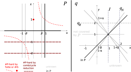
Figure 1: Complexity of the interlace polynomials $P$ and $q$. $\alpha=\sqrt{2}$, $\beta=1/\sqrt{2}$

Remark 4.1.

$P(\mu,0)$ and $P(1,\xi)$ are trivially solvable in polynomial time for any $\mu,\xi\in\tilde{\mathbb{Q}}$, as $P(G;\mu,0)=1$ and $P(G;1,\xi)=(1+\xi)^{|V|}$. ∎

Thus, on the thick black lines $x=0$ and $u=1$ in the left half of Figure 1, $P$ can be evaluated in polynomial time. By Lemma 2.3, these lines in the complexity map for $P$ correspond to the point $(1,1)$ and the line $x=y$, resp., in the complexity map for $q$, see the right half of Figure 1.

4.1 Identifying hard points

We want to establish Corollary 4.4 and Remark 4.5 which tell us, that $P$ is $\mathsf{\#P}$-hard to evaluate almost everywhere on the dashed hyperbola in Figure 1 and at $(0,1)$. To this end we collect known hardness results about the interlace polynomial.

Let $t(G;x,y)$ denote the Tutte polynomial of an undirected graph $G=(V,E)$. It may be defined by its state expansion as

$$t(G;x,y)=\sum_{B\subseteq E(G)}(x-1)^{r(E)-r(B)}(y-1)^{|B|-r(B)},$$ (4.1)

where $r(B)$ is the $\mathbb{F}_{2}$-rank of the incidence matrix of $G[B]=(V,B)$, the subgraph of $G$ induced by $B$. (Note that $r(B)$ equals the number of vertices of $G[B]$ minus the number of components of $G[B]$, which is the rank of $B$ in the cycle matriod of $G$.) For details about the Tutte polynomial we refer to standard literature [Tut84, BO92, Wel93]. The complexity of the Tutte polynomial has been studied extensively. In particular, the following result is known.

Theorem 4.2 ([Ver05]).

Evaluating the Tutte polynomial of planar graphs at $(\xi,\xi)$ is $\mathsf{\#P}$-hard for all $\xi\in\tilde{\mathbb{Q}}$ except for $\xi\in\{0,1,2,1\pm\sqrt{2}\}$.

We will profit from this by a connection between the interlace polynomial and the Tutte polynomial of planar graphs. This connection is established via medial graphs. For any planar graph $G$ one can build the oriented medial graph $\vec{G}_{m}$, find an Euler circuit $C$ in $\vec{G}_{m}$ and obtain the circle graph $H$ of $C$. The whole procedure can be performed in polynomial time. For details we refer to [EMS07]. We will use

Theorem 4.3 ([ABS04a, End of Section 7]; [EMS07, Theorem 3.1]).

Let $G$ be a planar graph, $\vec{G}_{m}$ be the oriented medial graph of $G$ and $H$ be the circle graph of some Euler circuit $C$ of $\vec{G}_{m}$. Then $q(H;2,y)=t(G;y,y)$. Thus we have $t(\upsilon,\upsilon)\preceq^{\mathtt{m}}P(\frac{1}{\upsilon-1},\upsilon-1)$, where $t(\upsilon,\upsilon)$ denotes the problem of evaluating the Tutte polynomial of a planar graph at $(\upsilon,\upsilon)$.

Proof.

See the references for $q(H;2,y)=t(G;y,y)$ and use Lemma 2.3. ∎

We set $\alpha=\sqrt{2}$ and $\beta=1/\sqrt{2}$. Let $B_{1}=\{\pm 1,\pm\beta,0\}$. Theorem 4.2 and Theorem 4.3 yield

Corollary 4.4.

Evaluating the vertex-nullity interlace polynomial $q_{N}$ is $\mathsf{\#P}$-hard almost everywhere. In particular, we have:

• The problem $q_{N}(2)$ is trivially solvable in polynomial time.

• For any $\upsilon\in\tilde{\mathbb{Q}}\setminus\{0,1,2,1\pm\alpha\}$ the problem $q_{N}(\upsilon)=q(2,\upsilon)$ is $\mathsf{\#P}$-hard. Or, in other words, for any $\mu\in\tilde{\mathbb{Q}}\setminus B_{1}$ the problem $P(\mu,1/\mu)$ is $\mathsf{\#P}$-hard. ∎

Remark 4.5.

$P(0,1)$ is $\mathsf{\#P}$-hard, as $P(G;0,1)$ equals the number of independent sets of $G$, which is $\mathsf{\#P}$-hard to compute [Val79]. ∎

4.2 Reducing to hard points

The cloning reduction allows us to spread the collected hardness over almost the whole plane: Combining Corollary 4.4 and Remark 4.5 with Proposition 3.4 we obtain

Proposition 4.6.

Let $B_{1}=\{\pm 1,\pm\beta,0\}$ and $B_{2}=\{0,-1,-2\}$ (as defined on Pages 4.3 and 3.4, resp.). Let $(\mu,\xi)\in((\tilde{\mathbb{Q}}\setminus B_{1})\cup\{0\})\times(\tilde{\mathbb{Q}}\setminus B_{2})$. Then $P(\mu,\xi)$ is $\mathsf{\#P}$-hard. ∎

This tells us that $P$ is $\mathsf{\#P}$-hard to evaluate at every point in the left half of Figure 1 not lying on one of the seven thick lines (three of which are solid gray ones, two of which are solid black ones, and two of which are dashed brown ones). Using the comb and cycle reductions we are able to reveal the hardness of the interlace polynomial $P$ on the lines $x=-1$ and $x=-2$:

Proposition 4.7.

For $\mu\in(\tilde{\mathbb{Q}}\setminus B_{1})\cup\{0\}$ the problem $P(\mu,-1)$ is $\mathsf{\#P}$-hard.

Proof.

For $\mu=0$ we use Proposition 3.8 and Remark 4.5. If $\mu\neq 0$, we can use Proposition 3.6, which yields $P(\mu,-1/\mu^{2})\preceq^{\mathtt{m}}P(\mu,-1)$. For $\mu=\pm 1$ this reduces $(\pm 1,-1)$ to itself. For $\mu=\pm\beta$ this reduces $(\beta,-2)$ to $(\beta,-1)$ and $(-\beta,-2)$ to $(-\beta,-1)$. For other $\mu$ this gives a reduction of some point, which is already known as $\mathsf{\#P}$-hard by Proposition 4.6, to $(\mu,-1)$. ∎

Proposition 4.8.

For $\mu\in(\tilde{\mathbb{Q}}\setminus B_{1})\cup\{0\}$ the problem $P(\mu,-2)$ is $\mathsf{\#P}$-hard.

Proof.

Use Proposition 3.8 and Proposition 4.6. ∎

4.3 Summing up

First we summarize our knowledge about $P$.

Theorem 4.9.

Let $\beta=1/\sqrt{2}$.

1. $P(\mu,\xi)$ is computable in polynomial time on the lines $\mu=1$ and $\xi=0$.

2. For $(\mu,\xi)\in(\tilde{\mathbb{Q}}\setminus\{-1,-\beta,\beta,1\})\times(\tilde{\mathbb{Q}}\setminus\{0\})$ the problem $P(\mu,\xi)$ is $\mathsf{\#P}$-hard.

Proof.

Summary of Remark 4.1, Proposition 4.6, Proposition 4.7, Proposition 4.8. The hardness of $P(0,-1)$ follows from Corollary 4.10. ∎

In particular we obtain the following corollary about the complexity of the independent set polynomial, which also follows from [AM07].

Corollary 4.10.

Evaluating the independent set polynomial $I(\lambda)=P(0,\lambda)=q(1,1+\lambda)$ is $\mathsf{\#P}$-hard at all $\lambda\in\tilde{\mathbb{Q}}$ except at $\lambda=0$, where it is computable in polynomial time.

Now we turn to the complexity of $q$, see also the right half of Figure 1.

Theorem 4.11.

The two-variable interlace polynomial $q$ is $\mathsf{\#P}$-hard to evaluate almost everywhere. In particular, we have:

1. $q(\xi,\upsilon)$ is computable in polynomial time on the line $\xi=\upsilon$.

2. Let $\xi\in\tilde{\mathbb{Q}}\setminus\{1\}$ and $x$ be an indeterminate. Then $q(\xi,1)$ is as hard as computing the whole polynomial $q(x,1)$.

3. $q(\xi,\upsilon)$ is $\mathsf{\#P}$-hard for all

   $$(\xi,\upsilon)\in\{(\xi,\upsilon)\in\tilde{\mathbb{Q}}^{2}\ |\ \upsilon\neq\pm(\xi-1)+1\ \text{and}\ \upsilon\neq\pm\sqrt{2}(\xi-1)+1\ \text{and}\ \upsilon\neq 1\}.$$

Proof of Theorem 4.11 (Sketch).

(1) and (3) follow from Remark 4.1 and Theorem 4.9 using Lemma 2.3. For $\xi\neq 1$, (3.5) gives $q(G_{k};\xi,1)=q(G;k(\xi-1)+1,1)$, which yields enough points for interpolation in the same way as in Proposition 3.4 using $k=1,2,3,\ldots$ This proves (2). ∎

Theorem 4.11 implies

Corollary 4.12.

Let $\beta=1/\sqrt{2}$. Evaluating the vertex-rank interlace polynomial $q_{R}(G;x)$ is $\mathsf{\#P}$-hard at all $\xi\in\tilde{\mathbb{Q}}$ except at $\xi=0,1-\beta,1+\beta$ (complexity open) and $\xi=2$ (computable in polynomial time). ∎

5 Inapproximability of the Independent Set Polynomial

Provided we can evaluate the independent set polynomial at some fixed point, vertex cloning (adding combs, resp.) allows us to evaluate it at very large points. In this section we exploit this to prove that the independent set polynomial is hard to approximate. Similar results are shown in [GJ07] for the Tutte polynomial.

Definition 5.1.

Let $\lambda\in\tilde{\mathbb{Q}}$ and $\varepsilon>0$. By a randomized $2^{n^{1-\varepsilon}}$-approximation algorithm for $I(\lambda)$ we mean a randomized algorithm, that, given a graph $G$ with $n$ nodes, runs in time polynomial in $n$ and returns $\tilde{I}(G;\lambda)\in\tilde{\mathbb{Q}}$ such that

$$\Pr[2^{-n^{1-\varepsilon}}I(G;\lambda)\leq\tilde{I}(G;\lambda)\leq 2^{n^{1-\varepsilon}}I(G;\lambda)]\geq\frac{3}{4}.$$

In [GJ07], (non)approximability in the weaker sense of (not) admitting an FPRAS is considered.

Definition 5.2.

Let $\lambda\in\tilde{\mathbb{Q}}$. A fully polynomial randomized approximation scheme (FPRAS) for $I(\lambda)$ is a randomized algorithm, that given a graph $G$ with $n$ nodes and an error tolerance $\varepsilon,0<\varepsilon<1$, runs in time polynomial in $n$ and $1/\varepsilon$ and returns $\tilde{I}(G;\lambda)\in\tilde{\mathbb{Q}}$ such that

$$\Pr[2^{-\varepsilon}I(G;\lambda)\leq\tilde{I}(G;\lambda)\leq 2^{\varepsilon}I(G;\lambda)]\geq\frac{3}{4}.$$

Lemma 5.3.

For every $\lambda\in\tilde{\mathbb{Q}}$, $0\neq|1+\lambda|\neq 1$, and every $\varepsilon$, $0<\varepsilon<1$, there is no randomized polynomial time $2^{n^{1-\varepsilon}}$-approximation algorithm for $I(\lambda)$ unless $\mathsf{RP}=\mathsf{NP}$.

Theorem 5.4.

For every $\lambda\in\tilde{\mathbb{Q}}\setminus\{0\}$ and every $\varepsilon$, $0<\varepsilon<1$, there is no randomized polynomial time $2^{n^{1-\varepsilon}}$-approximation algorithm (and thus also no FPRAS) for $I(\lambda)$ unless $\mathsf{RP}=\mathsf{NP}$.

Proof.

Lemma 5.3 gives the inapproximability at $\lambda\in\tilde{\mathbb{Q}}\setminus\{-2,-1,0\}$. By (3.6) we could turn an approximation algorithm for $I(-2)$ into an approximation algorithm for $I(2)$ which would imply $\mathsf{RP}=\mathsf{NP}$ by Lemma 5.3. For $I(-1)$ we use Theorem 3.7. ∎

Proof of Lemma 5.3.

Fix $\lambda\in\tilde{\mathbb{Q}},0\neq|1+\lambda|\neq 1$, and $\varepsilon$, $0<\varepsilon<1$. Assume we have a randomized $2^{n^{1-\varepsilon}}$-approximation algorithm $\mathcal{A}$ for $I(\lambda)$. Given a graph $G$, Theorem 3.3 and Theorem 3.5, resp., will allow us to evaluate the independent set polynomial at a point $\xi$ with $|\xi|$ that large, that an approximation of $I(G;\xi)$ can be used to recover the degree of $I(G;x)$, which is the size of a maximum independent set of $G$. As computing this number is $\mathsf{NP}$-hard, a randomized $2^{n^{1-\varepsilon}}$-approximation algorithm for $I(G;\lambda)$ would yield an $\mathsf{RP}$-algorithm for an $\mathsf{NP}$-hard problem, which implies $\mathsf{RP}=\mathsf{NP}$.

Let $G=(V,E)$ be a graph with $|V|=n$. We distinguish two cases. If $|1+\lambda|>1$, we choose a positive integer $l$ such that $(nl)^{1-\varepsilon}\geq n^{2}$ and with $\xi:=(1+\lambda)^{l}-1$ we have

$$|\xi|>2^{2(nl)^{1-\varepsilon}+n+2}.$$ (5.1)

As $\lambda$ and $\varepsilon$ are constant, this can be achieved by choosing $l=\mathsf{poly}(n)$. If $0<|1+\lambda|<1$, we choose a positive integer $l$ such that with $\xi:=\frac{\lambda}{(1+\lambda)^{l}}$ (5.1) holds. By Theorem 3.3 (Theorem 3.5, resp.) we have $I(G;\xi)=I(G_{l};\lambda)$ ($I(G;\xi)=(1+\lambda)^{-l|V|}I(G_{l};\lambda)$, resp.). Algorithm $\mathcal{A}$ returns on input $G_{l}$ within time $\mathsf{poly}(nl)=\mathsf{poly}(n)$ an approximation $\tilde{I}(G_{l};\lambda)$, such that with $\tilde{I}(G;\xi):=\tilde{I}(G_{l};\lambda)$ ($\tilde{I}(G;\xi):=\frac{\tilde{I}(G_{l};\lambda)}{(1+\lambda)^{l|V|}}$, resp.) we have

$$2^{-(nl)^{1-\varepsilon}}I(G;\xi)\leq\tilde{I}(G;\xi)\leq 2^{(nl)^{1-\varepsilon}}I(G;\xi)$$ (5.2)

with high probability.

Let $c$ be the size of a maximum independent set of $G$, and let $N$ be the number of independent sets of maximum size. We have

$$I(G;x)=Nx^{c}+\sum_{0\leq j\leq c-1}i(G;j)x^{j}$$

and thus

$$\begin{split}\Big{|}\frac{I(G;\xi)}{\xi^{c}}-N\Big{|}&\leq\sum_{0\leq j\leq c-1}i(G;j)|\xi|^{j-c}\\ &\leq c2^{n}|\xi|^{-1}\leq 2^{\log n+n}|\xi|^{-1}\overset{\eqref{eq:large_point}}{<}\frac{1}{2}.\end{split}$$ (5.3)

If we could evaluate $I(G;\xi)$ exactly, we could try all $c\in\{1,\ldots,n\}$ to find the one for which $\frac{I(G;\xi)}{\xi^{c}}$ is a good estimation for $N$, $1\leq N\leq 2^{n}$. This $c$ is unique as $|\xi|>2^{n^{2}}$. The following calculation shows that this is also possible using the approximation algorithm $\mathcal{A}$.

Using $\mathcal{A}$ we compute $\tilde{N}(\tilde{c}):=\frac{\tilde{I}(G;\xi)}{\xi^{\tilde{c}}}$ for all $\tilde{c}\in\{1,\ldots,n\}$. We claim that $c$ is the unique $\tilde{c}$ with

$$2^{-(nl)^{1-\varepsilon}-1}\leq\tilde{N}(\tilde{c})\leq 2^{(nl)^{1-\varepsilon}+n+1}.$$ (5.4)

Let us prove this claim. As $1\leq N\leq 2^{n}$ and by (5.3), we know that

$$\frac{1}{2}\leq\frac{I(G,\xi)}{\xi^{c}}\leq 2^{n+1}.$$ (5.5)

Thus, by (5.2), $\tilde{c}=c$ fulfills (5.4).

On the other hand, when $\tilde{c}\leq c-1$ we have

$$|\tilde{N}(\tilde{c})|\overset{\eqref{eq:approx},\eqref{eq:fraction_bounds}}{\geq}2^{-(nl)^{1-\varepsilon}-1}|\xi|\overset{\eqref{eq:large_point}}{>}2^{(nl)^{1-\varepsilon}+n+1}.$$

When $\tilde{c}\geq c+1$ we have $|\tilde{N}(\tilde{c})|<2^{-(nl)^{1-\varepsilon}-1}$ by similar arguments. This shows that any integer $\tilde{c},\tilde{c}\neq c,$ does not fulfill (5.4). Thus, $c$ can be found in randomized polynomial time using $\mathcal{A}$. ∎

References

• [ABCS00] Richard Arratia, Béla Bollobás, Don Coppersmith, and Gregory B. Sorkin. Euler circuits and DNA sequencing by hybridization. Discrete Applied Mathematics, 104(1-3):63–96, 15 August 2000.
• [ABS04a] Richard Arratia, Béla Bollobás, and Gregory B. Sorkin. The interlace polynomial of a graph. J. Comb. Theory Ser. B, 92(2):199–233, 2004.
• [ABS04b] Richard Arratia, Béla Bollobás, and Gregory B. Sorkin. A two-variable interlace polynomial. Combinatorica, 24(4):567–584, 2004.
• [AM07] Ilia Averbouch and J. A. Makowsky. The complexity of multivariate matching polynomials, February 2007. Preprint.
• [BM06] Markus Bläser and Johann Makowsky. Hip hip hooray for Sokal, 2006. Unpublished note.
• [BO92] Thomas Brylawski and James Oxley. The Tutte polynomial and its applications. In Neil White, editor, Matroid Applications, Encyclopedia of Mathematics and its Applications. Cambridge University Press, 1992.
• [Cou07] Bruno Courcelle. A multivariate interlace polynomial, 2007. Preprint, arXiv:cs.LO/0702016 v2.
• [EMS07] Joanna A. Ellis-Monaghan and Irasema Sarmiento. Distance hereditary graphs and the interlace polynomial. Comb. Probab. Comput., 16(6):947–973, 2007.
• [GJ07] Leslie Ann Goldberg and Mark Jerrum. Inapproximability of the Tutte polynomial. In STOC ’07: Proceedings of the 39th Annual ACM Symposium on Theory of Computing, pages 459–468, New York, NY, USA, 2007. ACM Press.
• [JVW90] F. Jaeger, D. L. Vertigan, and D. J. A. Welsh. On the computational complexity of the Jones and the Tutte polynomials. Math. Proc. Cambridge Philos. Soc., 108:35–53, 1990.
• [Sok05] Alan D. Sokal. The multivariate Tutte polynomial (alias Potts model) for graphs and matroids. In Bridget S. Webb, editor, Surveys in Combinatorics 2005. Cambridge University Press, 2005.
• [Tut84] W. T. Tutte. Graph Theory. Addison Wesley, 1984.
• [Val79] Leslie G. Valiant. The complexity of enumeration and reliability problems. SIAM Journal on Computing, 8(3):410–421, 1979.
• [Ver05] Dirk Vertigan. The computational complexity of Tutte invariants for planar graphs. SIAM Journal on Computing, 35(3):690–712, 2005.
• [Wel93] D. J. A. Welsh. Complexity: knots, colourings and counting. Cambridge University Press, New York, NY, USA, 1993.