Bichromatically driven double well: parametric perspective of the control landscape

Abstract

We numerically construct and study the control landscape of a $(\omega,2\omega)$ bichromatically driven double well in the presence of strong fields. The control landscape is obtained by correlating the overlap intensities between the floquet states and an initial phase space coherent state with the parametric motion of the quasienergies i.e., intensity-level velocity correlator. “Walls” of no control, robust under variations of the relative phase between the fields, are seen in the control landscape and associated with multilevel interactions involving chaotic floquet states.

The driven double well system is an important model and an ideal testbed for several schemes that have been suggested for controlling coherent superposition of quantum statesgh98 ; bsbook ; gdjh91 ; Holth92 ; fm93 ; sgsj04 . Starting with the demonstration of enhanced tunneling by Lin and Ballentinelb90 and coherent destruction of tunnelinggdjh91 (CDT) by Grossman et al. there has been a sustained interest in the driven double well due to its relevance in various areas like quantum computingqc , coherent controlbsbook , and quantum dotstkp07 . Many of the proposed control scenario involve few, carefully chosen, levels which provide valuable insights into the process. For example, the essence of CDT can be captured with a two-level floquet state analysisgp92 . However, such few-level schemes might be compromised due to several reasonscdb07 ; gb05 ; lgw94 ; nr05 and one of them, of interest in this work, has to do with the effect of chaos in the underlying phase spacegb05 . Typically, control in the presence of strong fields requires one to go beyond two (or few) level analysis since floquet states delocalized over the chaotic region of the classical phase space are expected to play an important rolegb05 ; lgw94 ; nr05 . Examples include work on bichromatically driven pendulumlgw94 and a recent analysis of the adiabatic passage technique for coherent population transfernr05 .

Despite the progress made towards understanding control in the presence of chaos, a comprehensive understanding of control in terms of the sensitivity to initial states, field strengths, and relative phases is still absent. The crucial object that one needs for such detailed understanding is the “control landscape” since the structure of the control landscape, amongst other things, can shed light on the robustness of the control strategiesrhr04 . To explain what we mean by a control landscape consider the Hamiltonian ($\hbar=1$)

$$H(x,p;t) = \frac{1}{2m}p^{2}+Bx^{4}-Dx^{2}+xf(t)$$ (1)

$$f(t) = \lambda_{1}\cos(\omega t)+\lambda_{2}\cos(2\omega t+\phi)$$

representing a driven double well. Our focus on bichromatic control is motivated by extensive studies that have shown the utility of such fields in addition to the possibility of the relative phase $\phi$ providing an additional control knobhcu07 . Owing to the periodicity of Eq. 1 the dynamics of an initial state $|z\rangle$ can be analyzedpg92 in terms of the floquet states $\{|\chi_{n}\rangle\}$ and the associated quasienergies $\{E_{n}\}$. The control landscape for fixed $\omega$ and a given $|z\rangle$ is the two-parameter space $(\lambda_{1},\lambda_{2})\equiv\bm{\lambda}$ exhibiting regions of control or lack thereof. An early example is the $(\lambda_{1},\omega)$ control plane for CDT which has been extended to construct the landscape for a bichromatically driven two-level systemdbm96 . Recentlysgsj04 , the difference between the quasienergies of the floquet states connected to the bare tunneling states of Eq. 1 has been used to map the control landscape.

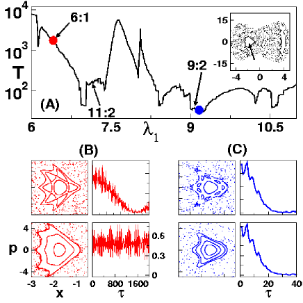
Figure 1: (Color online) (A) Decay time $T$ versus the field strength $\lambda_{1}$ for the coherent state, $|z\rangle\equiv|x_{0},p_{0}\rangle=|-1.5,0\rangle$, localized in the left regular island (indicated by an arrow in the inset showing the stroboscopic phase space at $\lambda_{1}=6.4$) and $\lambda_{2}=0$. Note the strong fluctuations in $T$ with the plateau regions around $\lambda_{1}=7.4$, and $9.2$. (B) and (C) top row shows the local phase space structure and survival probability for representative points $\lambda_{1}=6.4$ and $9.2$ respectively. The bottom row shows the effect of the weak control field (relative phase $\phi=0$) with strength $\lambda_{2}=0.2$ (B) and $\lambda_{2}=0.4$ (C) on the decay of $|z\rangle$.

The examples mentioned above clearly underscore the crucial role of avoided (exact) crossings between the floquet states. For strong driving fields the sheer number of such crossings, involving multiple floquet states, calls for an appropriate measure to construct the control landscape. Here we propose such a measure based on correlating the parametric motion of the floquet quasienergy levels (level velocities) with the overlap intensities $p_{zn}\equiv|\langle z|\chi_{n}\rangle|^{2}$. The overlap intensity-level velocity correlator was introduced by TomsovicToms96 , followed by detailed studieskct02 , as a sensitive measure of localization in phase space. We show, using Eq. 1 as example, that the correlator is an ideal measure for constructing and interpreting, perhaps quantitatively, the control landscape in the presence of strong fields.

In order to emphasize the role of chaos, consider the control problem of Eq. 1 with fixed parameter valueslb90 ; fm93 $m=1,D=10,B=0.5$ and, $\omega=6.07$. The double well supports about eight tunneling doublets and $\omega$ nearly corresponds to the energy separation between the ground and first excited states, neglecting the tunnel splittings. Since we are focusing on strong-field control, we choose $\lambda_{1}\in[6.0,11.0]$ for which the phase space shows two symmetry-related regular islands embedded in a chaotic sea. Earlier, Farrelly and Milligan have shownfm93 that control and suppression of tunneling can be achieved with $\lambda_{2}<\lambda_{1}=10$. In Fig. 1(A) the decay time $T$, in units of $2\pi/\omega$, of a coherent state $|z\rangle$ localized in the left regular island (cf. Fig. 1(A) inset) is shown as a function of $\lambda_{1}$ for $\lambda_{2}=0$. The decay time is infered from the first vanishing of the survival probability

$$S(\tau)\equiv|\langle z|\psi(\tau)\rangle|^{2}=\sum_{m,n}p_{zn}p_{zm}e^{-i(E_{n}-E_{m})\tau}$$ (2)

with the overlap intensities being $p_{zn}\equiv|\langle z|\chi_{n}\rangle|^{2}$. Despite the similar nature of the phase space, strong fluctuations in $T$ reflect the complicated dynamics of $|z\rangle$ as determined by the participation of floquet states and their phase space nature.

A natural question in the context of bichromatic control is as follows. For a given $T(\lambda_{1},\lambda_{2}=0)$, as in Fig. 1(A), what choice of the $2\omega$-field strength $\lambda_{2}$ and phase $\phi$ will suppress the decay? Motivated by recent studiesmes06 one suspects that the local phase phase structure about $|z\rangle$ is an important factor. To this end, in Fig. 1(B) and (C) we show the local phase space structure near the left regular island and the associated $S(\tau)$ for two representative values of $\lambda_{1}$. In case (B) a prominent $6$:$1$ nonlinear resonance is observed. On addition of a weak second field $\lambda_{2}=0.2$ the nonlinear resonance disappears and $S(\tau)$ does not decay to zero. On the other hand in case (C) a $9$:$2$ resonance is observed for $\lambda_{2}=0$ which vanishes at $\lambda_{2}=0.4$. However $S(\tau)$ is hardly effected although in both cases the discrete symmetry is broken ($\phi=0$) upon addition of the $2\omega$-field. Similar insensitivity to the local phase space structure occurs in the vicinity of regions exhibiting plateaus in Fig. 1(A). In other words, attempts to control the decay of $|z\rangle$ in the plateau regions is bound to be difficult. Such plateau regions, near regular-chaotic avoided crossings, have been observedtu94 in the context of chaos-assisted tunneling. Thus, chaotic floquet states are expected to be key for understanding the features in Fig. 1(A).

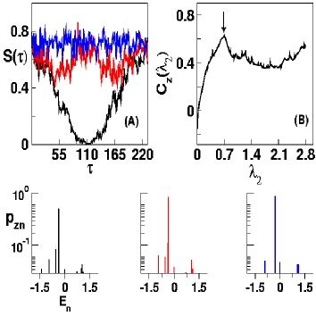
Figure 2: (Color online) (A) Survival probability $S(\tau)$ of $|z\rangle=|-1.5,0\rangle$ with $\lambda_{1}=10$, $\phi=0$ and varying $\lambda_{2}=0$ (black), $0.7$ (red), and $2.5$ (blue). (B) The overlap intensity-level velocity correlator (cf. Eq. 3) is shown as a function of $\lambda_{2}$. $C_{z}(\bm{\lambda})$ exhibits a peak around $\lambda_{2}=0.7$ indicating substantial localization and agreeing with the behaviour of $S(\tau)$ in (A). (Bottom panel) Overlap intensities for $\lambda_{2}=0,0.7$ and, $2.5$ (left to right) indicate breaking of the symmetry for $\lambda_{2}\neq 0$.

Several questions arise at this juncture. What is the precise role of the chaotic states for control? Are the plateaus robust for varying $\lambda_{2}$ and $\phi$? In order to address these questions we motivate the intensity-level velocity correlatorToms96 and show that a simple criterion on the correlator highlights the regimes of control. The floquet states and quasienergies of Eq. 1 are parametrically dependent on the field strengths i.e., $E_{n}=E_{n}(\bm{\lambda})$ and $|\chi_{n}\rangle=|\chi_{n}(\bm{\lambda})\rangle$. Thus the response of a floquet state to the $2\omega$-field is measured by the parametric derivative, also known as level velocity, $\partial E_{n}/\partial\lambda_{2}$. At the same time the decay dynamics of a coherent state $|z\rangle$ is dominated by floquet states that have appreciable overlap with $|z\rangle$ (cf. Eq. 2). Therefore, floquet states $|\chi_{n}\rangle$ with substantial overlap $p_{zn}$ and large $\partial E_{n}/\partial\lambda_{2}$ are expected to be important in controlling the dynamics of $|z\rangle$. The qualitative argument can be made quantitative by introducing the overlap intensity-level velocity correlatorToms96

$$C_{z}(\lambda_{1},\lambda_{2})=\frac{1}{\sigma_{z}\sigma_{E}}\left\langle p_{zn}\frac{\partial E_{n}(\bm{\lambda})}{\partial\lambda_{2}}\right\rangle_{n}$$ (3)

where $\sigma_{z}^{2}$ and $\sigma_{E}^{2}$ are the local variances of $p_{zn}$ and $\partial E_{n}/\partial\lambda_{2}$ respectively. The average in Eq. 3 is over all the floquet states but the dominant contributions are expected to come from a finite number of them according to the qualitative argument above. In order to keep the level velocities to be zero centered, the mean is subtracted and $C_{z}(\bm{\lambda})$ is rescaled to a unitless quantity with unit variance, making it a true correlation coefficientToms96 . In effect, $C_{z}(\bm{\lambda})$ provides information on groups of states exhibiting common localization characteristics and is thus a quantitative measure for deviations from ergodicity.

Utility of the correlator can be illustrated with the example discussed previouslyfm93 with $\lambda_{1}=10$ (fixed), $\lambda_{2}=2.5$ and, $\phi=0$. For the chosen parameters the phase space symmetry is broken and the suppression of tunneling is evident from Fig. 2(A). However, Fig. 2(B) shows that $C_{z}(\bm{\lambda})$ as a function of $\lambda_{2}$ rises rapidly for small $\lambda_{2}$, peaks at $\lambda_{2}\approx 0.7$, and varies slowly for larger values. Interestingly, similar values of $C_{z}(\bm{\lambda})$ at $\lambda_{2}=0.7$ and $\lambda_{2}=2.5$ suggests comparable extent of localization in phase space. Indeed Fig. 2(A) shows that the tunneling is significantly suppressed already around $\lambda_{2}=0.7$. Note that for $\lambda_{2}=2.5$ the symmetry between the two regular islands is broken markedly resulting in the considerable suppression of tunneling seen in Fig. 2(A). In contrast, for $\lambda_{2}=0.7$ the symmetry breaking is hardly perceptible in the phase space and yet there is a strong effect on the quantum dynamics. This has been notedlgw94 before and Fig. 2 shows that the correlator is capable of capturing such effects.

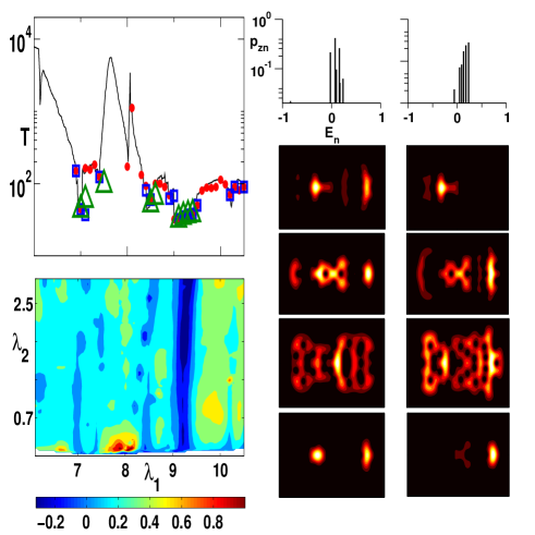
Figure 3: (Color online) The left column shows the control landscape (bottom panel) compared to the decay time plot (top panel, solid line as in Fig. 1(A)). In the decay time plot only points that are least affected upon adding the $2\omega$-field with strengths $\lambda_{2}=0.2$ (red circles), $0.7$ (blue squares), and $2.1$ (green triangles) are shown. Note that the regions where there is a lack of control correspond to the plateaus with $C_{z}(\bm{\lambda})\leq 0$. The middle and right columns show the overlap intensities for $\lambda_{2}=0$ and $2.1$ respectively with $\lambda_{1}=9.2$ (fixed). Multiple state interactions involving chaotic floquet states are involved. The Husimi representationslb90 of the states are shown below the corresponding intensity plots with the axis range being identical to that of the inset in Fig. 1(A). See text for details.

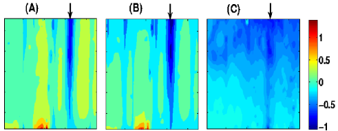
Figure 4: (Color online) Control landscape (axes range as in Fig. 3) corresponding to (A) $\phi=\pi/4$, (B) $\pi/3$, and (C) $\pi/2$. In (C) most of the landscape exhibits $C_{z}(\bm{\lambda})\leq 0$ indicating lack of control. Regions of control gradually emerge in (B) and (C) (see also Fig. 3 for $\phi=0$). Note the robustness of the “wall” of no control around $\lambda_{1}\approx 9.2$ (indicated by arrows).

We now construct the control landscape for the entire range of $\lambda_{1}$ shown in Fig. 1(A). Since $2\omega$-field is the control, the intensity-velocity correlator in Eq. 3 is evaluated at a given point $(\lambda_{1},\lambda_{2})$ using the response of the floquet states with changing field strength $\lambda_{2}$. The resulting control landscape is shown in Fig. 3 together with the decay time data of Fig. 1(A) for relative phase $\phi=0$. The decay time plot shows regions which cannot be controlled by the $2\omega$-field which, interestingly, correspond precisely to the plateaus in Fig. 1(A). A noteworthy feature of the control landscape is the existence of “walls” of no control which are characterized by $C_{z}(\bm{\lambda})\leq 0$. In particular, such a wall at $\lambda_{1}\approx 9.2$ seems to be quite robust and persists for fairly large values of $\lambda_{2}$. Other such regions around $\lambda_{1}\approx 7.0$, and $8.2$ seem to break up for higher values of $\lambda_{2}$. Our analysis reveals that in the wall regions the dynamics of $|z\rangle$ is dominated by multiple floquet states delocalized in the phase space. An example of the multiple floquet contributions, as evident from the overlaps, and the chaotic nature of the associated Husimi representationslb90 is shown in Fig. 3. Note that the participation of the chaotic floquet states at $\lambda_{2}=0$ (no control field) persists even for large $\lambda_{2}$. Hence, using the symmetry breaking property of the $2\omega$-field for control purposes is not very effective when chaotic floquet states are participating in the dynamics. On the other hand regions with $C_{z}(\bm{\lambda})>0$ indicate varying extent of control of the decay. It is interesting to note that the ealier analysisfm93 happens to be in a region away from such walls of no control!

The effect of varying the relative phase $\phi$ on the control landscape is shown in Fig. 4. The case $\phi=\pi/2$ is shown in Fig. 4(C) and one observes that $C_{z}(\bm{\lambda})\leq 0$ over most of the landscape which indicates very little control. This is consistent with the fact that the combined driving field is symmetric for $\phi=\pi/2$. The control landscape for $\phi=\pi/3$, and $\pi/4$ are also shown in Fig. 4(B) and (A) respectively. Note that decreasing $\phi$ from the symmetric value of $\pi/2$ gradually leads to regions of control. However, it is intriguing to see that the wall of no control seen in Fig. 3 for $\lambda_{1}\approx 9.2$ is present for all the values of $\phi$ shown here. For systems with effective $\hbar\ll 1$ one expects several such plateau regions and the effectiveness of the control would depend sensitively on the initial state and field parameters.

In conclusion, we have constructed the control landscape for the bichromatically driven double well in the presence of strong fields using a novel and highly sensitive measure. A simple criterion on the correlator is able to distinguish between regions of control and regions of no control. Lack of control is associated with the involvement of chaotic floquet states and the robustness of such regions of no control reitratescdb07 the need to excercise care in proposing finite-level control schemes in the presence of strong fields. We are currently exploring the usefulness of the correlator, applicable in the presence of adiabatic fields as well, as a tool in formulating local control strategies.

SK gratefully acknowledges useful discussions with Prof. Harshawardhan Wanare. Astha Sethi is funded by a Fellowship from the University Grants Commission, India.

References

- (1) M. Grifoni and P. Hänggi, Phys. Rep. 304, 229 (1998).
- (2) M. Shapiro and P. Brumer, Principles of the Quantum Control of Molecular Processes (Wiley, New York, 2003); K. Bergmann, H. Theuer, and B. Shore, Rev. Mod. Phys. 70, 1003 (1998).
- (3) F. Grossmann, T. Dittrich, P. Jung, and P. Hänggi, Phys. Rev. Lett. 67, 516 (1991).
- (4) M. Holthaus, Phys. Rev. Lett. 69, 1596 (1992); R. Bavli and H. Metiu, Phys. Rev. Lett. 69, 1986 (1992); S. Ya. Kilin, P. R. Berman, and T. M. Maevskaya, Phys. Rev. Lett. 76, 3297 (1996); J. Y. Shin, Phys. Rev. E 54, 289 (1996); A. Igarashi and H. Yamada, Chem. Phys. 327, 395 (2006).
- (5) D. Farrelly and J. A. Milligan, Phys. Rev. E 47, R2225 (1993).
- (6) N. Sangouard, S. Guérin, M. Aminat-Talab, and H. R. Jauslin, Phys. Rev. Lett. 93, 223602 (2004).
- (7) W. A. Lin and L. E. Ballentine, Phys. Rev. Lett. 65, 2927 (1990).
- (8) M. Ndong, D. Lauvergnat, X. Chapuisat, and M. Desouter-Lecomte, J. Chem. Phys. 126, 244505 (2007); U. Troppmann, C. Gollub, and R. de Vivie-Riedle, New J. Phys. 8, 100 (2006); S. Suzuki, K. Mishima, and K. Yamashita, Chem. Phys. Lett. 410, 358 (2005).
- (9) A. F. Terzis, S. Kosionis, and E. Paspalakis, J. Phys. B: At. Mol. Opt. Phys. 40, S331 (2007).
- (10) J. M. G. Llorente and J. Plata, Phys. Rev. A 45, R6958 (1992).
- (11) T. Cheng, H. Darmawan, and A. Brown, Phys. Rev. A 75, 013411 (2007); D. Sugny et al., Phys. Rev. A 74, 043419 (2006).
- (12) J. Gong and P. Brumer, Annu. Rev. Phys. Chem. 56, 1 (2005); S. Kohler, R. Utermann, P. Hänggi, and T. Dittrich, Phys. Rev. E 58, 7219 (1998).
- (13) M. Latka, P. Grigolini and B. J. West, Phys. Rev. E 50, R3299 (1994).
- (14) K. Na and L. E. Reichl, Phys. Rev. A 72, 013402 (2005); Chaos, Solitons and Fractals, 25, 185 (2005).
- (15) H. A. Rabitz, M. M. Hsieh, and C. M. Rosenthal, Science 303, 1998 (2004).
- (16) F. Ehlotzky, Phys. Rep. 345, 175 (2001); S. Huang, C. Chandre, and T. Uzer, J. Phys. B: At. Mol. Opt. Phys. 40, F181 (2007); L. Sirko and P. M. Koch, Phys. Rev. Lett. 89, 274101 (2002); S. Denisov, L. Morales-Molina, S. Flach, and P. Hänggi, Phys. Rev. A 75, 063424 (2007); V. Constantoudis and C. A. Nicolaides, J. Chem. Phys. 122, 084118 (2005); I. Vrábel and W. Jakubetz, J. Chem. Phys. 118, 7366 (2003); V. S. Batista and P. Brumer, Phys. Rev. Lett. 89, 143201 (2002).
- (17) J. Plata and J. M. G. Llorente, J. Phys. A: Math. Gen. 25, L303 (1992).
- (18) Y. Dakhnovskii, R. Bavli, and H. Metiu, Phys. Rev. B 53, 4657 (1996).
- (19) S. Tomsovic, Phys. Rev. Lett. 77, 4158 (1996).
- (20) N. R. Cerruti, S. Keshavamurthy, and S. Tomsovic, Phys. Rev. E 68, 056205 (2003); S. Keshavamurthy, N. R. Cerruti and S. Tomsovic, J. Chem. Phys. 117, 4168 (2002); A. Lakshminarayan, N. R. Cerruti, and S. Tomsovic, Phys. Rev. E 63, 016209 (2000).
- (21) S. Keshavamurthy, Phys. Rev. E 72, 045203(R) (2005); S. Wimberger, P. Schlagheck, C. Eltschka, and A. Buchleitner, Phys. Rev. Lett. 97, 043001 (2006).
- (22) S. Tomsovic and D. Ullmo, Phys. Rev. E 50, 145 (1994).