State-Relevant Maxwell’s Equation from Kaluza-Klein Theory

Abstract

We study a five-dimensional perfect fluid coupled with Kaluza-Klein (KK) gravity. By dimensional reduction, a modified form of Maxwell’s equation is obtained, which is relevant to the equation of state of the source. Since the relativistic magnetohydrodynamics (MHD) and the 3-dimensional formulation are widely used to study space matter, we derive the modified Maxwell’s equations and relativistic MHD in 3+1 form. We then take an ideal Fermi gas as an example to study the modified effect, which can be visible under high density or high energy condition, while the traditional Maxwell’s equation can be regarded as a result in the low density and low temperature limit. We also indicate the possibility to test the state-relevant effect of KK theory in a telluric laboratory.

I Introduction

A unified formulation of Einstein’s theory of gravitation and Maxwell’s theory of electromagnetism in four-dimensional (4D) spacetime was first proposed by Kaluza and Klein using a five-dimensional (5D) geometry Kaluza ; Klein . A free test particle in 5D KK spacetime shows its electricity in the reduced 4D spacetime when it moves along the fifth dimension. Moreover a 5D dust field coupled with KK gravity can curve the 5D spacetime in such a way that it provides exactly the source of the electromagnetic field in the 4D spacetime after the reduction KK . In this paper we study the coupling of a 5D perfect fluid with KK gravity. It turns out that the 5D Einstein’s equation with a source gives a modification of Maxwell’s equation (see in section II), which can show its state-relevant effect on high-density or high-temperature condition (see in section IV). Thus this effect provides intriguing possibilities for the experimental test of the KK theory. Note that the KK theory which we are considering is purely classical. The KK theory has also been studied from the particle physics point of view (see e.g. Kubyshin ), which can show its effects in high energy scale of $TeV$. Whereas the energy scale needed for testing our state-relevant effect is only around $keV$.

In order to reveal the physical implication of the modification more clearly, both the modified Maxwell’s equations and the corresponding general relativistic MHD are reformulated in 3+1 form (see in section III). The formalism is also useful for evolving numerically a relativistic MHD fluid in a spacetime characterized by a strong gravitational field. Taking an ideal Fermi gas as an example, the modification term is studied as a function of degeneracy and temperature parameters (see in section IV). Moreover the modification terms for different components of the perfect fluid may be different. This would result in a net charge excess in high-temperature plasma. Recall that the the electrical neutrality of atoms and of bulk matter has been examined precisely by a number of experiments Gillies . However, in those experiments, either the objects considered are not ionized, or the ions in the objects cannot be regarded as a perfect fluid. Therefore, these experiments cannot provide definite opposite evidence to the classical KK theory since they do not satisfy our premise. But they do cast some doubts on it. Taking account of the state-relevant character, we suggest high-temperature plasma in earth laboratory or dense-matter white dwarf in outer space as candidates to test the possible effects of the modified Maxwell’s equation.

II Kaluza-Klein gravity coupled with 5D perfect fluid

Using a 5D geometry, Kaluza and Klein proposed a unified formulation of gravity and electromagnetism in 4D spacetime Kaluza ; Klein . The original KK theory assumed the so-called“Cylinder Condition”, which means that there exists a space-like killing vector field $\xi^{a}$ on the 5D spacetime ($\hat{M},\hat{g}_{ab}$) duff -yang . Note that the abstract index notation Wald is employed throughout the paper and the signature of the five-metric is of the convention $(-,+,+,+,+)$. In addition, Kaluza also demanded that $\xi^{a}$ is normalized, i.e.,

$$\phi\equiv\hat{g}_{ab}\xi^{a}\xi^{b}=1\ .$$ (1)

Later research shows that the Ansatz (1) may be dropped out and the $\phi$ may play a key role in the study of cosmology uzan ; BR ; Wehus ; Mohamm . Being an extra dimension, the orbits of $\xi^{a}$ are geometrically circles. The physical consideration that any displacement in the usual “physical” 4D spacetime (denoted as $M$) should be orthogonal to the extra dimension implies that the “physical” 4D metric should be defined as

$$g_{ab}=\hat{g}_{ab}-\phi^{-1}\xi_{a}\xi_{b}\ ,$$ (2)

and the projection operator onto $M$ is

$$g^{a}_{~{}b}=\hat{g}^{a}_{~{}b}-\phi^{-1}\xi^{a}\xi_{b}\ .$$ (3)

For practical calculation, it is convenient to take a coordinate system $\{z^{M}=(x^{\mu},y)|\mu=0,1,2,3\}$ with coordinate basis $(e_{M})^{a}=\{(e_{\mu})^{a},(e_{5})^{a}\}$ on $\hat{M}$ adapted to $\xi^{a}$, i.e., $(e_{5})^{a}=(\frac{\partial}{\partial y})^{a}=\xi^{a}$. Then the 5-metric components $\hat{g}_{MN}$ take the form

$$\hat{g}_{MN}=\left(\begin{array}[]{cc}g_{\mu\nu}+\phi B_{\mu}B_{\nu}&\phi B_{\mu}\\ \phi B_{\nu}&\phi\\ \end{array}\right),$$ (4)

where $\hat{g}_{\mu 5}\equiv\phi B_{\mu}$. So, locally, the “physical” spacetime can be understood as a 4-manifold $M$ with the coordinates $\{x^{\mu}\}$ endowed with the metric $g_{ab}$. The whole theory is governed by the 5D Einstein-Hilbert action

$$S_{G}=-\frac{1}{2\hat{k}}\int_{\hat{M}}d^{4}xdy\sqrt{-\hat{g}}\hat{R}\ .$$ (5)

Suppose the range of the fifth coordinate to be $0\leq y\leq L$ and denote $k=\hat{k}/L$. Let $B_{\mu}=fA_{\mu},f^{2}=2k$, then equation (5) becomes a coupling action on $M$ as

$$\hat{S}_{G}=\int_{M}d^{4}x\sqrt{-g}\sqrt{\phi}\left(-\frac{1}{2k}R+\frac{1}{4}\phi F_{ab}(A)F^{ab}(A)\right)\ ,$$ (6)

where $R$ is the curvature scalar of $g_{ab}$ on $M$ and $F_{ab}(A)\equiv 2\partial_{[a}A_{b]}$. Thus, it results in a 4D gravity $g_{ab}$ coupled to an electromagnetic field $A_{a}$ and a scalar field $\phi$. It is clear that, under the Ansatz (1), 5D KK theory unifies the Einstein’s gravity and the source-free Maxwell’s field in the standard formulism.

Now we consider a 5D perfect fluid

$$\hat{T}_{ab}=(\hat{p}+\hat{\mu})\hat{V}_{a}\hat{V}_{b}+\hat{p}\hat{g}_{ab}\ .$$ (7)

The 5-velocity $\hat{V}^{a}$ can be projected onto the “physical” spacetime $(M,g_{ab})$ as

$$u^{a}\equiv g^{a}_{~{}b}\hat{V}^{b}=\hat{V}^{\mu}(e_{\mu})^{a}-(B_{\mu}\hat{V}^{\mu})(e_{5})^{a}\ .$$ (8)

Note that we have $\hat{V}^{a}\hat{V}_{a}=-1$, hence it is easy to show that

$$\hat{V}^{\mu}\hat{V}_{\mu}\equiv\hat{g}_{ab}u^{a}u^{b}=g_{ab}\hat{V}^{a}\hat{V}^{b}=-1-\frac{Q^{2}}{\phi}\ ,$$ (9)

where $Q\equiv\hat{V}_{5}=\hat{g}_{5a}\hat{V}^{a}$ represents the electric charge in $M$ KK . The energy-momentum tensor can be projected on M as $\tilde{T}_{ab}\equiv g_{a}^{~{}c}g_{b}^{~{}d}\hat{T}_{cd}$. In order to obtain the observed 4D energy-momentum tensor $T_{ab}$ on $M$, we have to integrate $\tilde{T}_{ab}$ along the extra dimension. In the light of (8) and (9) we obtain

$$T_{ab}=(\mu+p)v_{a}v_{b}+pg_{ab}\ ,$$ (10)

where

$$p = \hat{p}\sqrt{\phi}L,$$

$$\mu = \frac{\hat{\mu}L(Q^{2}+\phi)}{\sqrt{\phi}}+\hat{p}L\frac{Q^{2}}{\sqrt{\phi}},$$

$$v_{a} = \frac{u_{a}}{\sqrt{-\hat{V}^{\mu}\hat{V}_{\mu}}}\ .$$ (11)

It is clear that $T_{ab}$ is the energy-momentum tensor of a 4D perfect fluid in $M$, where $\mu$ and $p$ are respectively the energy density and pressure density observed by a comoving observer in $M$.

We now consider the reduction of 5D Einstein’s equation

$$\hat{R}_{ab}-\frac{1}{2}\hat{g}_{ab}\hat{R}=\hat{k}\hat{T}_{ab}\ ,$$ (12)

which is equivalent to

$$\hat{R}_{ab}=\hat{k}(\hat{T}_{ab}-\frac{1}{3}\hat{T}^{c}_{c}\hat{g}_{ab})\ .$$ (13)

It is not difficult to show from Eq. (5) that the components of the 5D Ricci tensor $\hat{R}_{ab}$ can be expressed as Wehus

$$\hat{R}_{55}=\frac{1}{2}k\phi^{2}F^{\sigma\rho}F_{\sigma\rho}-\frac{1}{2}\nabla^{\mu}\nabla_{\mu}\phi+\frac{1}{4\phi}(\nabla^{\mu}\phi)\nabla_{\mu}\phi\ ,$$ (14)

$$\hat{R}_{\mu 5} = \frac{f}{2}(\phi\nabla^{\nu}F_{\mu\nu}+\frac{3}{2}F_{\mu\nu}\nabla^{\nu}\phi)$$ (15)

$$+B_{\mu}\left(\frac{1}{2}k\phi^{2}F^{\sigma\rho}F_{\sigma\rho}-\frac{1}{2}\nabla^{\nu}\nabla_{\nu}\phi+\frac{1}{4\phi}(\nabla^{\nu}\phi)\nabla_{\nu}\phi\right)\ ,$$

$$\hat{R}_{\mu\nu} = R_{\mu\nu}-k\phi F^{\sigma}_{\ \mu}F_{\sigma\nu}-\frac{1}{2\phi}\nabla_{\mu}\nabla_{\nu}\phi+\frac{1}{4\phi^{2}}(\nabla_{\mu}\phi)\nabla_{\nu}\phi$$ (16)

$$+B_{\mu}B_{\nu}\left(\frac{1}{2}k\phi^{2}F^{\sigma\rho}F_{\sigma\rho}-\frac{1}{2}\nabla^{\sigma}\nabla_{\sigma}\phi+\frac{1}{4\phi}(\nabla^{\sigma}\phi)\nabla_{\sigma}\phi\right)$$

$$+\frac{f}{2}B_{\mu}(\phi\nabla^{\sigma}F_{\nu\sigma}+\frac{3}{2}F_{\nu\sigma}\nabla^{\sigma}\phi)$$

$$+\frac{f}{2}B_{\nu}(\phi\nabla^{\sigma}F_{\mu\sigma}+\frac{3}{2}F_{\mu\sigma}\nabla^{\sigma}\phi)\ ,$$

where $\nabla_{a}$ is the 4D covariant derivative operator associated with $g_{ab}$. Substituting Eq. (14) into Eq. (13), we obtain a coupling equation for the matter fields as

$$\frac{1}{2}k\phi^{2}F^{ab}F_{ab}=\sqrt{\phi}\nabla^{a}\nabla_{a}\sqrt{\phi}+k\sqrt{\phi}\mu\left(1-\frac{2\phi}{3(\phi+Q^{2})}\right)+k\sqrt{\phi}p\frac{Q^{2}-\phi}{3(Q^{2}+\phi)}\ .$$ (17)

Substituting Eq. (15) into Eq. (13) and using Eq. (17), we obtain an electromagnetic field equation with source as

$$\phi\nabla^{b}F_{ab}+\frac{3}{2}F_{ab}\nabla^{b}\phi=\tilde{\gamma}(1+\frac{p}{\mu})J_{a}\ ,$$ (18)

here we have defined $\tilde{\gamma}\equiv\sqrt{(1+Q^{2})/(\phi+Q^{2})}$, $\rho\equiv\frac{f\mu Q}{\sqrt{\phi(1+Q^{2})}}$ and $J^{a}\equiv\rho v^{a}$ KK . Substituting Eq. (16) into Eq. (13) and using Eq. (17) and (18), we obtain a 4D Einstein’s equation with source as

$$G_{ab} = \frac{k}{\sqrt{\phi}}\left((\mu+p)v_{a}v_{b}+g_{ab}p+\phi^{3/2}(F^{~{}c}_{a}F_{bc}-\frac{1}{4}g_{ab}F^{cd}F_{cd})\right.$$ (19)

$$\left.-\frac{1}{k}(g_{ab}\nabla^{c}\nabla_{c}\sqrt{\phi}-\nabla_{a}\nabla_{b}\sqrt{\phi})\right),$$

where $G_{ab}$ is the Einstein tensor of $g_{ab}$. More generally, if the 5D perfect fluid consists of $m$ components, $\hat{T}_{ab}$ then reads

$$\hat{T}_{ab}=\sum_{\eta=1}^{m}\left((\hat{p}_{\eta}+\hat{\mu}_{\eta})\hat{V}_{a}(\eta)\hat{V}_{b}(\eta)+\hat{p}_{\eta}\hat{g}_{ab}\right)\ .$$ (20)

By similar calculations, Eqs. (17)-(19) become respectively

$$\frac{1}{2}k\phi^{2}F^{ab}F_{ab} = \sqrt{\phi}\nabla^{a}\nabla_{a}\sqrt{\phi}+k\sqrt{\phi}\sum_{\eta=1}^{m}\mu(\eta)\left(1-\frac{2\phi}{3(\phi+Q(\eta)^{2})}\right)$$ (21)

$$+k\sqrt{\phi}\sum_{\eta=1}^{m}p(\eta)\frac{Q(\eta)^{2}-\phi}{3(Q(\eta)^{2}+\phi)}\ ,$$

$$\phi\nabla^{b}F_{ab}+\frac{3}{2}F_{ab}\nabla^{b}\phi=\sum_{\eta=1}^{m}\tilde{\gamma}(\eta)\left(1+\frac{p(\eta)}{\mu(\eta)}\right)J_{a}(\eta)\ ,$$ (22)

$$G_{ab} = \frac{k}{\sqrt{\phi}}\left(\sum_{\eta=1}^{m}((\mu(\eta)+p(\eta))v_{a}(\eta)v_{b}(\eta)+g_{ab}p(\eta))+\phi^{3/2}(F^{~{}c}_{a}F_{bc}-\frac{1}{4}g_{ab}F^{cd}F_{cd}\right.$$ (23)

$$\left.-\frac{1}{k}(g_{ab}\nabla^{c}\nabla_{c}\sqrt{\phi}-\nabla_{a}\nabla_{b}\sqrt{\phi})\right)\ .$$

It is interesting to see the results when $\phi\equiv 1$. Eqs. (17)-(19) become respectively

$$\frac{1}{2}kF^{ab}F_{ab}=k\mu\left(1-\frac{2}{3(1+Q^{2})}\right)+kp\frac{Q^{2}-1}{3(Q^{2}+1)}\ ,$$ (24)

$$\nabla^{b}F_{ab}=(1+\frac{p}{\mu})J_{a}\ ,$$ (25)

$$G_{ab}=k(T_{ab}^{({\mathrm{fluid}})}+T_{ab}^{({\mathrm{em}})})\ ,$$ (26)

where $T_{ab}^{({\mathrm{fluid}})}\equiv(\mu+p)v_{a}v_{b}+pg_{ab}$ and $T_{ab}^{({\mathrm{em}})}=F_{a}^{~{}c}F_{bc}-\frac{1}{4}g_{ab}F^{cd}F_{cd}$ are respectively the usual energy-momentum tensors of 4D perfect fluid and electromagnetic field. Eq. (26) is the standard 4D Einstein’s equation while Eq. (25) is not the same as the standard 4D Maxwell’s equation $\nabla^{b}F_{ab}=J_{a}$. The new term $(1+\frac{p}{\mu})$ brings an effective charge which can be considered as a state-relevant effect, as will be discussed later. We thus call Eq. (25) the state-relevant Maxwell’s equation.

III Maxwell’s equations and relativistic MHD in 3+1 form

Since relativistic MHD is widely used to study space matter and 3D formulation is frequently applied to dealing with specific issues Baumgarte , we now derive the modified results of Maxwell’s equations and relativistic MHD in 3+1 form. The 4D spacetime $M$ is foliated into a family of non-intersecting spacelike three-surfaces $\Sigma$, which arise, at least locally, as level surfaces of a scalar time function $t$. The spatial metric $\gamma_{ab}$ on the three-dimensional hypersurfaces $\Sigma$ is induced by the spacetime metric $g_{ab}$ according to

$$\gamma_{ab}=g_{ab}+n_{a}n_{b}\ ,$$ (27)

where $n^{a}$ is the unit normal vector to the slices and thus $n_{a}=-\alpha\nabla_{a}t$. Here the normalization factor $\alpha$ is called the lapse function. The time vector $t^{a}$ is dual to the foliation 1-form $\nabla_{a}t$ and can be decomposed as

$$t^{a}=\alpha n^{a}+\beta^{a}\ ,$$ (28)

where the shift vector $\beta$ is spatial, i.e., $n_{a}\beta^{a}=0$. Since the extrinsic curvature $K_{ab}$ of $\Sigma$ can be written as

$$K_{ab}=-\nabla_{a}n_{b}-n_{a}a_{b}\ ,$$ (29)

where $a_{a}\equiv n^{b}\nabla_{b}n_{a}$, the divergence of $n^{a}$ satisfies

$$\nabla_{a}n^{a}=-K\ ,$$ (30)

here $K$ is the trace of $K_{ab}$.

Firstly we write the modified Maxwell’s equations in 3+1 form. The Faraday tensor $F^{ab}$ can be decomposed as

$$F^{ab}=n^{a}E^{b}-n^{b}E^{a}+\epsilon^{abc}B_{c}\ ,$$ (31)

where $E^{a}$ and $B^{a}$ are the electric and magnetic fields observed by a normal observer $n^{a}$. Both fields are purely spatial, whereby

$$E^{a}n_{a}=0\ \ and\ \ B^{a}n_{a}=0\ ,$$ (32)

and the three-dimensional Levi-Civita symbol $\epsilon_{abc}$ is defined by

$$\epsilon_{abc}=n^{d}\epsilon_{dabc}\ \ or\ \ \epsilon^{abc}=n_{d}\epsilon^{dabc}\ .$$ (33)

The electromagnetic current four-vector $J^{a}$ is decomposed as

$$J^{a}=n^{a}\rho_{e}+j^{a}\ ,$$ (34)

where $\rho_{e}$ and $j^{a}$ are the charge density and 3-current as observed by a normal observer $n^{a}$. Note that $j^{a}$ is purely spatial, i.e., $j^{a}n_{a}=0$. With these definitions, the modified Maxwell’s equations (17), (18) and $\nabla_{[a}F_{bc]}=0$ can be cast into 3+1 form as

$$k\phi^{2}(B^{2}-E^{2}) = \sqrt{\phi}(D^{a}D_{a}\sqrt{\phi}-(\alpha^{-1}(\partial_{t}-\mathcal{L}_{\beta}))^{2}\sqrt{\phi}$$ (35)

$$+K\alpha^{-1}(D_{a}\sqrt{\phi})(D^{a}\ln\alpha)(\partial_{t}-\mathcal{L}_{\beta})\sqrt{\phi})$$

$$+k\sqrt{\phi}\mu\left(1-\frac{2\phi}{3(\phi+Q^{2})}\right)+k\sqrt{\phi}p\frac{Q^{2}-\phi}{3(\phi+Q^{2})},$$

$$D_{a}E^{a} = \phi^{-1}(\tilde{\gamma}(1+\frac{p}{\mu})\rho_{e}-\frac{3}{2}E^{a}D_{a}\phi),$$ (36)

$$\phi\mathcal{L}_{t}E^{a} = \phi(\alpha KE^{a}+\mathcal{L}_{\beta}E^{a}+\epsilon^{abc}D_{b}(\alpha B_{c}))$$ (37)

$$-\alpha\tilde{\gamma}(1+\frac{p}{\mu})j^{a}+\frac{3}{2}\alpha(\epsilon^{abc}B_{b}D_{c}\phi-E^{a}\alpha^{-1}(\partial_{t}-\mathcal{L}_{\beta})\phi)\ ,$$

$$D_{a}B^{a} = 0\ ,$$ (38)

$$\mathcal{L}_{t}B^{a} = -\epsilon^{abc}D_{b}(\alpha E_{c})+\alpha KE^{a}+\mathcal{L}_{\beta}B^{a}\ ,$$ (39)

here $\mathcal{L}_{\beta}$ denotes the Lie-derivative along $\beta^{a}$ and $D_{a}$ is the covariant derivative operator associated to $\gamma_{ab}$. Note that the Lie-derivative of a spacelike tensor $A^{a\cdots b}_{~{}c\cdots d}$ along $s^{a}$ is defined conventionally as $\tilde{\mathcal{L}}_{s}A^{a\cdots b}_{~{}c\cdots d}\equiv\gamma^{a}_{e}\cdots\gamma^{b}_{f}\gamma^{g}_{c}\cdots\gamma^{h}_{d}\mathcal{L}_{s}A^{e\cdots f}_{~{}g\cdots h}$, and we write $\tilde{\mathcal{L}}_{s}$ as $\mathcal{L}_{s}$ for short. Note also that the formula $n^{b}\nabla_{b}n_{a}=a_{a}=D_{a}ln\alpha$ is used in the above calculation 1982 . If one considered a 5D perfect fluid consisting of $m$ components, the terms $\tilde{\gamma}(1+\frac{p}{\mu})\rho_{e}$ and $\tilde{\gamma}(1+\frac{p}{\mu})j^{a}$ in Eqs. (36) and (37) would be replaced by $\sum_{\eta=1}^{m}\tilde{\gamma}(\eta)(1+\frac{p(\eta)}{\mu(\eta)})\rho_{e}(\eta)$ and $\sum_{\eta=1}^{m}\tilde{\gamma}(\eta)(1+\frac{p(\eta)}{\mu(\eta)})j^{a}$. When $\phi\equiv 1$, one can see from Eq. (36) that $\tilde{\rho}_{e}\equiv(1+p/\mu)\rho_{e}$ is the effective charge density serving as the source of the electric field. This effective charge density is state-relevant, i.e., it is dependent on $p/\mu$. Its significance will be discussed later.

Secondly we rewrite modified relativistic MHD in 3+1 form. Note that the total energy-momentum tensor in $M$ can be read off from the right hand side of Eq. (19) as

$$T^{ab}\equiv T^{ab}_{({\mathrm{fluid}})}+\tilde{T}^{ab}_{({\mathrm{em}})}+T^{ab}_{(\phi)}\ ,$$ (40)

where

$$\tilde{T}^{ab}_{({\mathrm{em}})} \equiv \phi^{3/2}T^{ab}_{({\mathrm{em}})}=\phi^{3/2}(F^{ac}F^{b}_{~{}c}-\frac{1}{4}g^{ab}F^{cd}F_{cd})\ ,$$ (41)

$$T^{ab}_{(\phi)} \equiv -\frac{1}{k}(g^{ab}\nabla^{c}\nabla_{c}\sqrt{\phi}-\nabla^{a}\nabla^{b}\sqrt{\phi})\ .$$ (42)

It is straightforward to see that gravity

$$\nabla_{b}T^{ab}_{({\mathrm{em}})}=F^{ac}\nabla^{b}F_{bc}\ .$$ (43)

In the light of Eqs. (27)-(33), we obtain the 3+1 form

$$\nabla_{b}T^{ab}_{({\mathrm{em}})} = n^{a}(-KE^{2}+\alpha^{-1}E_{b}(\mathcal{L}_{t}-\mathcal{L}_{\beta})E^{b}-\alpha^{-1}\epsilon^{bcd}E_{b}D_{c}(\alpha B_{d}))$$ (44)

$$-E^{a}D_{b}E^{b}+\epsilon^{abc}B_{c}\alpha^{-1}(\mathcal{L}_{t}-\mathcal{L}_{\beta}-\alpha K)E_{b}$$

$$+\alpha^{-1}B_{b}D^{a}(\alpha B^{b})-\alpha^{-1}B_{b}D^{b}(\alpha B^{a})\ ,$$

$$T^{ab}_{({\mathrm{em}})}\nabla_{b}\phi^{3/2} = \frac{3\sqrt{\phi}}{2}\left(\frac{1}{2}(B^{2}+E^{2})(D^{a}\phi+n^{a}\alpha^{-1}(\partial_{t}-\mathcal{L}_{\beta})\phi)\right.$$ (45)

$$-(E^{a}E^{b}+B^{a}B^{b})D_{b}\phi$$

$$\left.+E_{c}B_{d}(n^{a}\epsilon^{bcd}D_{b}\phi+\epsilon^{acd}\alpha^{-1}(\partial_{t}-\mathcal{L}_{\beta})\phi)\right),$$

here $E^{2}\equiv E_{a}E^{a}$ and $B^{2}\equiv B_{a}B^{a}$. Recall that the relation between three-dimensional Riemann tensor ${}^{3}R_{abc}^{d}$ and 4D one $R_{abc}^{d}$ reads

$${}^{3}R_{abc}^{d}=\gamma_{a}^{e}\gamma_{b}^{f}\gamma_{c}^{l}\gamma_{m}^{d}R_{efl}^{m}-2K_{c[a}K_{b]}^{~{}d}.$$ (46)

Using

$$(\nabla_{a}\nabla_{b}-\nabla_{b}\nabla_{a})\nabla^{c}\sqrt{\phi}=-R_{abd}^{~{}~{}~{}c}\nabla^{d}\sqrt{\phi},$$ (47)

a lengthy but straightforward calculation gives

$$\nabla_{b}T^{ab}_{(\phi)} = \frac{1}{2k\sqrt{\phi}}\left.(^{3}R^{ab}D_{b}\phi+\alpha^{-1}(D_{b}K^{ab}-D^{a}K)(\partial_{t}-\mathcal{L}_{\beta})\phi\right.$$ (48)

$$-(D^{b}\phi)(\alpha^{-1}(\mathcal{L}_{t}-\mathcal{L}_{\beta})K^{a}_{~{}b}+K^{ac}K_{bc}$$

$$+D^{a}D_{b}\ln\alpha+(D^{a}\ln\alpha)D_{b}\ln\alpha)$$

$$+n^{a}(\alpha^{-1}((\partial_{t}-\mathcal{L}_{\beta})\phi)(-K^{bc}K_{bc}+D^{b}D_{b}\ln\alpha+a^{2}$$

$$+\alpha^{-1}(\partial_{t}-\mathcal{L}_{\beta})K)+(D_{b}K^{bc})D_{c}\phi-(D^{b}K)D_{b}\phi$$

$$\left.-K_{bc}(D^{b}\phi)D^{c}\ln\alpha)\right),$$

where ${}^{3}R^{ab}$ is the three-dimensional Ricci tensor and $a^{2}\equiv a^{a}a_{a}$. For a perfect fluid, the energy-momentum tensor $T^{ab}_{({\mathrm{fluid}})}$ can also be written as

$$T^{ab}_{({\mathrm{fluid}})}=\rho hv^{a}v^{b}+pg^{ab}\ ,$$ (49)

where $\rho$ is the rest-mass density as observed by an observer co-moving with the fluid $v^{a}$, $p$ is the pressure and $h$ the specific enthalpy

$$h=1+\epsilon+p/\rho.$$ (50)

Hence one has $\mu=(1+\epsilon)\rho$. The local conservation of the 4D Einstein tensor $G^{ab}$ leads to

$$\nabla_{b}(T^{ab}/\sqrt{\phi})=0\ .$$ (51)

We assume that $T^{ab}_{(\phi)}$ does not contribute to the number of baryons. Thus we have the conservation of baryons as

$$\nabla_{a}(\rho v^{a})=0\ ,$$ (52)

which is decomposed into 3+1 form as

$$D_{a}(\rho\tilde{v}^{a})+\alpha^{-1}(\partial_{t}-\mathcal{L}_{\beta})(\rho W)-\rho WK+\rho\tilde{v}^{a}D_{a}\ln\alpha=0,$$ (53)

where $\tilde{v}^{a}\equiv v^{a}-Wn^{a}$. The equation for the conservation of energy is obtained by contracting Eq. (51) with $n_{b}$ as

$$H = \alpha^{-1}(\partial_{t}-\mathcal{L}_{\beta})p-W\rho(\tilde{v}^{a}D_{a}h+W\alpha^{-1}(\partial_{t}-\mathcal{L}_{\beta})h)$$ (54)

$$-\rho h(W\alpha^{-1}(\partial_{t}-\mathcal{L}_{\beta})W+\tilde{v}^{a}D_{a}W$$

$$+W\tilde{v}^{a}D_{a}\ln\alpha-K_{ab}\tilde{v}^{a}\tilde{v}^{b}),$$

and the Euler equation is obtained by projecting Eq. (51) onto $\Sigma$ as

$$\rho h\tilde{v}^{a}D_{b}\tilde{v}^{a} = \rho h(2WK^{ab}\tilde{v}_{b}-W^{2}D^{a}\ln\alpha)-\rho hW\alpha^{-1}(\mathcal{L}_{t}-\mathcal{L}_{\beta})\tilde{v}^{a}$$ (55)

$$-\rho\tilde{v}^{a}(W\alpha^{-1}(\partial_{t}-\mathcal{L}_{\beta})h+\tilde{v}^{b}D_{b}h)-D^{a}p-M^{a},$$

where

$$H \equiv \phi^{3/2}(-KE^{2}+\alpha^{-1}E_{a}(\mathcal{L}_{t}-\mathcal{L}_{\beta})E^{a}-\alpha^{-1}\epsilon^{abc}E_{a}D_{b}(\alpha B_{c}))$$ (56)

$$+\frac{\sqrt{\phi}}{2}(B^{2}+E^{2})\alpha^{-1}(\partial_{t}-\mathcal{L}_{\beta})\phi+\sqrt{\phi}\epsilon^{abc}E_{a}B_{b}D_{c}\phi$$

$$+\frac{1}{2k\sqrt{\phi}}(\alpha^{-1}(\partial_{t}-\mathcal{L}_{\beta})\phi(-K^{ab}K_{ab}+D^{a}D_{a}\ln\alpha+a^{2}$$

$$+\alpha^{-1}(\partial_{t}-\mathcal{L}_{\beta})K)+(D_{a}K^{ab})D_{b}\phi-(D^{a}K)D_{a}\phi)$$

$$-\frac{W}{2\phi}(\mu+p)\tilde{v}^{b}D_{b}\phi+\frac{1}{2k\phi}(D_{a}\phi)(\alpha^{-1}(\mathcal{L}_{t}-\mathcal{L}_{\beta})D^{a}\sqrt{\phi}$$

$$-K_{ab}D^{b}\sqrt{\phi})+\frac{1}{2\phi}\alpha^{-1}(-W^{2}(\mu+p)+p-\frac{1}{k}(D^{a}D_{a}\sqrt{\phi}$$

$$+K\alpha^{-1}(\partial_{t}-\mathcal{L}_{\beta})\sqrt{\phi}+(D_{a}\sqrt{\phi})D^{a}\ln\alpha))(\partial_{t}-\mathcal{L}_{\beta})\phi,$$

and

$$M^{a} \equiv +\sqrt{\phi}(\frac{1}{2}(B^{2}+E^{2})D^{a}\phi-(E^{a}E^{b}+B^{a}B^{b})D_{b}\phi$$ (57)

$$+\epsilon^{abc}E_{b}B_{c}\alpha^{-1}(\partial_{t}-\mathcal{L}_{\beta})\phi)-\phi^{3/2}E^{a}D_{b}E^{b}$$

$$+\phi^{3/2}\alpha^{-1}(\epsilon^{abc}B_{c}(\mathcal{L}_{t}-\mathcal{L}_{\beta}-\alpha K)E_{b}+B_{b}D^{a}(\alpha B^{b})-B_{b}D^{b}(\alpha B^{a}))$$

$$+\frac{1}{2k\sqrt{\phi}}\left({}^{3}R^{ab}D_{b}\phi+\alpha^{-1}(D_{b}K^{ab}-D^{a}K)(\partial_{t}-\mathcal{L}_{\beta})\phi\right)$$

$$-(D^{b}\phi)\left(\alpha^{-1}(\mathcal{L}_{t}-\mathcal{L}_{\beta})K^{a}_{~{}b}+K^{ac}K_{bc}+D^{a}D_{b}\ln\alpha+(D^{a}\ln\alpha)D_{b}\ln\alpha\right)$$

$$-\frac{1}{2\phi}(\mu+p)(\tilde{v}^{b}D_{b}\phi+W\alpha^{-1}(\partial_{t}-\mathcal{L}_{\beta})\phi)\tilde{v}^{a}-\frac{1}{2\phi}pD^{a}\phi$$

$$+\frac{1}{2k\phi}(D^{a}\phi)\left(D^{b}D_{b}\sqrt{\phi}-(\alpha^{-1}(\partial_{t}-\mathcal{L}_{\beta}))^{2}\sqrt{\phi}\right.$$

$$\left.+K\alpha^{-1}(\partial_{t}-\mathcal{L}_{\beta})\sqrt{\phi}+(D_{b}\sqrt{\phi})D^{b}\ln\alpha\right)$$

$$-\frac{1}{2k\phi}\left((D_{b}\phi)D^{a}D^{b}\sqrt{\phi}+(\alpha^{-1}(\partial_{t}-\mathcal{L}_{\beta})\sqrt{\phi})K^{ab}D_{b}\phi\right.$$

$$\left.-(\alpha^{-1}(\partial_{t}-\mathcal{L}_{\beta})\phi)D^{a}(\alpha^{-1}(\partial_{t}-\mathcal{L}_{\beta})\sqrt{\phi})\right),$$

here $(\alpha^{-1}(\partial_{t}-\mathcal{L}_{\beta}))^{2}\sqrt{\phi}$ denotes $\alpha^{-1}(\partial_{t}-\mathcal{L}_{\beta})(\alpha^{-1}(\partial_{t}-\mathcal{L}_{\beta})\sqrt{\phi})$. Note that Eqs. (53), (54) and (55) comprise the basic formulas for the modified relativistic MHD in three-dimensional form. In the special case $\phi\equiv 1$, we have

$$H = -KE^{2}+\alpha^{-1}E_{a}(\mathcal{L}_{t}-\mathcal{L}_{\beta})E^{a}-\alpha^{-1}\epsilon^{abc}E_{a}D_{b}(\alpha B_{c}),$$ (58)

$$M^{a} = -E^{a}D_{b}E^{b}+\alpha^{-1}\epsilon^{abc}B_{c}(\mathcal{L}_{t}-\mathcal{L}_{\beta}-\alpha K)E_{b}$$ (59)

$$+\alpha^{-1}\left(B_{b}D^{a}(\alpha B^{b})-B_{b}D^{b}(\alpha B^{a})\right),$$

which accord with the conventional form Baumgarte .

IV Discussion on the effective charge

From the state-relevant Maxwell’s equation (25) and its 3+1 form Eq. (36), we can see that $\tilde{\rho}_{e}\equiv(1+p/\mu)\rho_{e}$ is the effective charge density of a perfect fluid. Such effective charge density is relevant to the equation of state of the fluid and its rationality should be carefully checked. In this section, we adopt an ideal Fermi gas as an example to see under what condition can the modified term $p/\mu$ show visible effect. We employ in terms of the dimensionless degeneracy and temperature parameters

$$\eta=\frac{\tilde{\mu}}{k_{B}T},\ \ \ \beta=\frac{k_{B}T}{mc^{2}},$$ (60)

where $\tilde{\mu}$ is the chemical potential, $m$ is the mass of the fermion, and $k_{B}$ is the Boltzmann constant. The gas is degenerate for $\eta\gg 0$ while nondegenerate for $\eta\ll 0$. On the other hand, the gas is extremely relativistic for $\beta\gg 1$ while nonrelativistic for $\beta\ll 1$ fermi . The zero of energy for the particles is chosen so that the thermodynamic potential reads

$$\Omega=-Vk_{B}T\int\frac{gd^{3}\tilde{p}}{h^{3}}\ln\left[1+\exp\frac{\tilde{\mu}-\varepsilon}{k_{B}T}\right],$$ (61)

where $\tilde{p}$ is the momentum, $g$ is the statistical weight, and

$$\varepsilon=\sqrt{(\tilde{p}c)^{2}+(mc^{2})^{2}}-mc^{2}$$ (62)

is the kinetic energy. The number density $n$, pressure $p$, and internal energy density $E$ (per volume) of an ideal Fermi gas are respectively

$$n = K\beta^{3/2}\left[F_{1/2}(\eta,\beta)+\beta F_{3/2}(\eta,\beta)\right],$$ (63)

$$p = mc^{2}K\beta^{5/2}\left[\frac{2}{3}F_{3/2}(\eta,\beta)+\frac{1}{3}\beta F_{5/2}(\eta,\beta)\right],$$ (64)

$$E = mc^{2}K\beta^{5/2}\left[F_{3/2}(\eta,\beta)+\beta F_{5/2}(\eta,\beta)\right],$$ (65)

where $K=4\sqrt{2}\pi g(mc/h)^{3}$, and the Fermi integral is

$$F_{k}(\eta,\beta)\equiv\int_{0}^{+\infty}\frac{z^{k}(1+\frac{1}{2}\beta z)^{1/2}dz}{e^{z-\eta}+1}\ \ \ \ (k>-1).$$ (66)

Then we have

$$\frac{p}{\mu}=\frac{p}{E+nmc^{2}}=\frac{1}{3+{3F_{1/2}(\eta,\beta)}/({2\beta F_{3/2}(\eta,\beta)+\beta^{2}F_{5/2}(\eta,\beta)})}.$$ (67)

The relation between $p/\mu$ and $(\eta,\beta)$ is shown in Fig. 1. One can see clearly that both degenerate and relativistic conditions can lead to the value of $p/\mu$ comparable to $1/3$ (which is the value of $p/\mu$ for radiation).

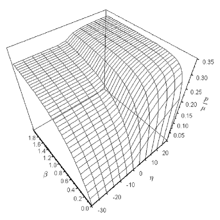
Figure 1: Modified term $p/\mu$ as a function of degeneracy parameter $\eta$ and relativistic parameter $\beta$.

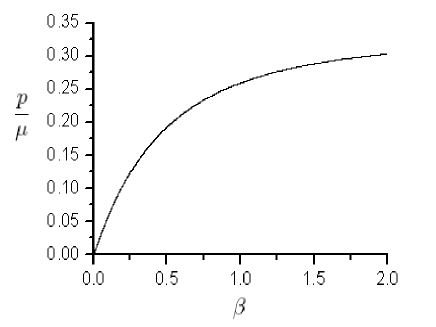
Figure 2: Modified term $p/\mu$ as a function of relativistic parameter $\beta$ in nondegenerate condition $\eta=-30$.

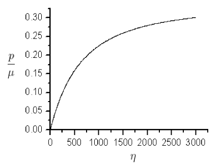
Figure 3: Modified term $p/\mu$ as a function of degeneracy parameter $\eta$ in nonrelativistic condition $\beta=10^{-9}$.

Now we study the two kinds of conditions respectively. For a nondegenerate ideal Fermi gas (for example $\eta=-30$), the value of $p/\mu$ is drawn from nonrelativistic ($\beta=0$) to relativistic ($\beta=2$) regime in Fig. 2. It is obvious that we need not to go to extremely relativistic condition since $p/\mu$ is already close to $1/3$ when $\beta=2$. In the specific calculation for an electron gas, we set $p/\mu=0.002$ when $k_{B}T=1~{}\mathrm{keV}$. This result indicates the possibility to test the theory in earth laboratory. For a non-degenerate electron gas at $T=273K$, one may estimate the modification term as $p/\mu\sim k_{B}T/m_{e}c^{2}\sim 10^{-8}$. On the other hand, in the experiments on the equality of the electric charges of proton and electron, these charges in a conductor are found to be equal within $10^{-19}$ or better (see e.g. Stover ). However, the proton system in a conductor cannot be seen as a perfect fluid and hence does not satisfy our premise. Hence the effective charges of protons in a conductor cannot be directly obtained by our modified equations. So, those experiments are not in severe contradiction with the KK theory. For similar reason, the experiments reported in Ref.Gillies cannot provide definite opponent evidence to the KK theory either. But this kind of experiments do cast some doubts on the classical KK theory. Note that both the electron system and the ion system could be regarded as perfect fluid in high-temperature plasma. In a thermal equilibrium state the electron and ion in a plasma have the same temperature. Hence they would have different values of $p/\mu$. Actually the value of $p/\mu$ for ion is much smaller than the one for electron when $k_{B}T$ takes value from $\mathrm{keV}$ to $\mathrm{MeV}$. It turns out that the two important physical parameters for the description of plasma–Debye length and plasma frequency PP have to be modified in our 5D theory as

$$\lambda_{D}=\left[\frac{\epsilon_{0}k_{B}T}{n_{e}e^{2}(1+p_{e}/\mu_{e})}\right]^{\frac{1}{2}}\ ,$$ (68)

and

$$\omega_{p}=\left[\frac{n_{e}e^{2}(1+p_{e}/\mu_{e})}{m_{e}\epsilon_{0}}\right]^{\frac{1}{2}}\ ,$$ (69)

where $n_{e}$ is the number density of electron and $\epsilon_{0}$ the permittivity of vacuum. Since the electromagnetic wave whose frequency is lower than $\omega_{p}$ will be reflected while others can transmit through the plasma, the plasma frequency can be measured accurately Xu . Therefore it is possible to test the prediction from the 5D KK theory in earth laboratory. For a degenerate idea Fermi gas, the relation between $p/\mu$ and $\eta$ is demonstrated in Fig. 3. Recall that the white dwarf is known to resist the gravity by an electronic degenerate pressure. It is also possible to test the 5D theory by certain relevant phenomena in outerspace.

Note that the vacuum polarization in quantum electrodynamics (QED) also leads to an effective charge of a point-like particle Greiner ; Peskin . So the effective charge viewpoint does not merely come from the KK theory. For the Fermi gas in KK theory, the larger the density and the temperature, the larger the effective charge factor $\tilde{\rho}_{e}/\rho_{e}$, which approaches to $4/3$ as a limit. Whereas for QED, the higher the energy scale (or shorter distance), the larger the effective charge $e_{\mathrm{eff}}/e$, which approaches to infinity as a limit. Therefore the state-relevant Maxwell’s equation and QED give similar results of larger effective charges. However, the state-relevant effect in KK theory is a pure classical effect due to the extra dimension of spacetime, whereas the QED effect is a quantum effect irrespective of any extra dimension. So one does not expect them to be the same. It is easy to distinguish the two effects by comparing their characters.

In Summary, the coupling of 5D perfect fluid to KK gravity is fully studied. The 4D effective equations of this 5D coupling system are derived. In particular, the modified Maxwell’s equation which is relevant to the equation of state of the source is obtained. To facilitate applications, we also derive the 3+1 form of the modified Maxwell’s equations and the relativistic MHD. It turns out that the effective charge density in the KK theory can be written as $\tilde{\rho}_{e}\equiv(1+p/\mu)\rho_{e}$. Moreover, using an ideal Fermi gas model, we study the modification term $p/\mu$ as a function of degeneracy parameter $\eta$ and the relativity parameter $\beta$. It reveals that the traditional Maxwell’s equation is the low density and low temperature limit of the state-relevant Maxwell’s equation. We thus indicate the possibility to test the state-relevant effect both in earth laboratory and in astrophysical phenomena.

References

- (1) T. Kaluza, Sitzungsber. Preuss. Akad. Wiss. Phys. Mat. Klasse 1921, 966 (1921).
- (2) O. Klein, Z. Phys. 37, 895 (1926).
- (3) Y. Ma and J. Wu, Int. J. Mod. Phys. A19, 5043 (2004).
- (4) Y. A. Kubyshin, Arxiv preprint: hep-ph/0111027.
- (5) C. S. Unnikrishnan and G. T. Gillies, Metrologia 41, S125 (2004).
- (6) M.J. Duff, B.E.W. Nilsson, and C.N. Pope, Phys. Rep. 130, 1 (1986).
- (7) J.M. Overduin and P.S. Wesson, Phys. Rep. 283, 303 (1997).
- (8) X. Yang, Y. Ma, J. Shao, and W. Zhou, Phys. Rev. D68, 024006 (2003).
- (9) R.M. Wald, General Relativity (The University of Chicago Press, 1984).
- (10) J-P. Uzan, Rev. Mod. Phys. 75, 403 (2003).
- (11) P.J.E. Peebles and B. Ratra, Rev. Mod. Phys. 75, 559 (2003).
- (12) I.K. Wehus and F. Ravndal, Int. J. Mod. Phys. A19, 4671 (2004).
- (13) N. Mohammedi, Phys. Rev. D65, 104018 (2002).
- (14) T.W. Baumgarte and S.L. Shapiro, Astrophys. J. 585, 921 (2003).
- (15) K.S. Thorne and D.A. MacDonale, Month. Not. R. Astr. Soc. 198, 345 (1982).
- (16) C.W. Misner, K.S. Thorne and J.A. Wheeler, Gravitation, (Freeman, New York, 1973).
- (17) J.A. Miralles and K.A. Van Riper, Astrophys. J. Suppl. S 105, 407 (1996).
- (18) R.W. Stover, T.I. Moran and J.W. Trischka, Phys. Rev. 164, 1599 (1967).
- (19) J.A. Bittencourt, Fundamentals of Plasma Physics, (Springer, 2004).
- (20) R. Xu, Introduction to Astrophysics, (Peking University Press, 2006, in Chinese).
- (21) W. Greiner and J. Reinhardt, Quantum Electrodynamics, Second Edition, (Springer, 1994).
- (22) M.E. Peskin and D.V. Schroeder, An Introduction to Quantum Field Theory, (Addison-Wesley Publishing Company, 1997).