arXiv:0707.4472

DESY 07-110

MIT-CTP-3851

Exact marginality in open string field theory: a general framework

Michael Kiermaier¹ and Yuji Okawa²

¹ Center for Theoretical Physics
Massachusetts Institute of Technology
Cambridge, MA 02139, USA
mkiermai@mit.edu

² DESY Theory Group
Notkestrasse 85
22607 Hamburg, Germany
yuji.okawa@desy.de

Abstract

We construct analytic solutions of open bosonic string field theory for any exactly marginal deformation in any boundary conformal field theory when properly renormalized operator products of the marginal operator are given. We explicitly provide such renormalized operator products for a class of marginal deformations which include the deformations of flat D-branes in flat backgrounds by constant massless modes of the gauge field and of the scalar fields on the D-branes, the cosine potential for a space-like coordinate, and the hyperbolic cosine potential for the time-like coordinate. In our construction we use integrated vertex operators, which are closely related to finite deformations in boundary conformal field theory, while previous analytic solutions were based on unintegrated vertex operators. We also introduce a modified star product to formulate string field theory around the deformed background.

1 Introduction

String field theory can potentially be a background-independent formulation of string theory. In the current formulation of string field theory, however, we first need to choose one conformal field theory (CFT) describing a consistent background of string theory. The crucial question is then whether other string backgrounds can be described as classical solutions of string field theory. In particular, for each exactly marginal deformation of the CFT, we expect to have a family of solutions in string field theory labeled by the deformation parameter.

Recent remarkable developments in analytic methods of open string field theory [5]–[26] enabled us to address this question in a concrete setting. Analytic solutions for marginal deformations when operator products of the marginal operator are regular were constructed to all orders in the deformation parameter in [17, 18] for open bosonic string field theory [27] and in [19, 20, 22] for open superstring field theory [28]. When the operator product of the marginal operator is singular, analytic solutions were constructed to third order in the deformation parameter in [18]. Recently, analytic solutions for the deformation generated by the zero mode of the gauge field were constructed in [21] by a different approach and extended to open superstring field theory in [25]. While the equation of motion is satisfied to all orders in the deformation parameter, a closed form expression for a solution satisfying the reality condition on the string field has not been presented in [21, 25]. For earlier study of marginal deformations in string field theory, see [29]–[42].

In this paper, we present a procedure to construct a solution satisfying the reality condition in open bosonic string field theory for any exactly marginal deformation in any boundary CFT when properly renormalized operator products of the marginal operator are given. The analytic solutions in [17, 18] were constructed using unintegrated vertex operators and $b$-ghost insertions. Our strategy is to use integrated vertex operators, which are closely related to finite deformations in boundary CFT. We assume several properties of the properly renormalized operator products of the marginal operator. Since the identification of a set of assumptions which are sufficient for the construction of a solution is one of the main points of the paper, we will explain these assumptions in detail in the following. We will then present our solutions.

1.1 Assumptions

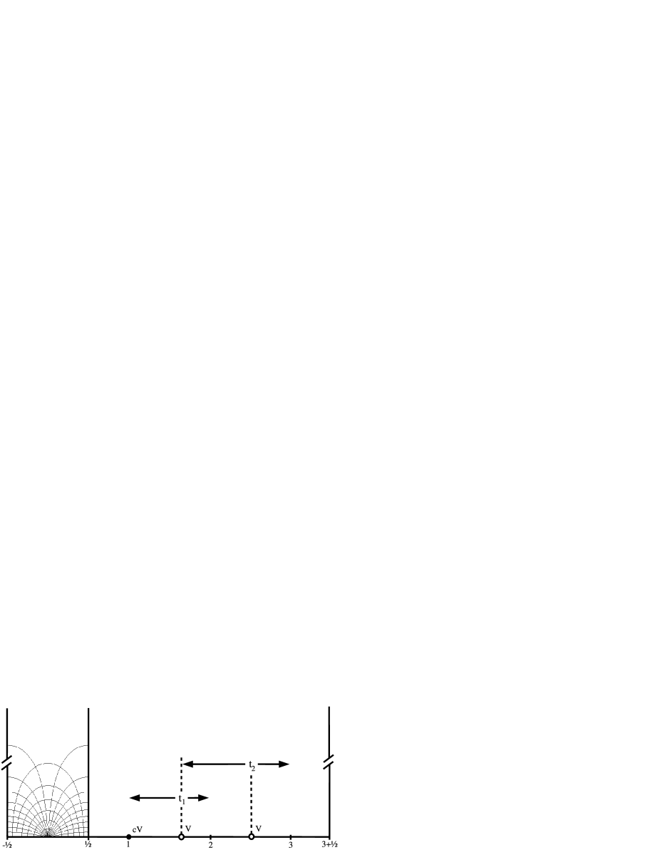
When there exists an exactly marginal deformation in a given boundary CFT, we have a family of consistent boundary conditions labeled by the deformation parameter which we denote by $\lambda$. Consider the boundary CFT on the upper-half plane and suppose that we change boundary conditions on a segment of the boundary between $a$ and $b$. Since the new boundary condition is also conformal, an integral of the BRST current along a contour vanishes if both end points of the contour lie inside the region between $a$ and $b$. By $C(t_{f},\,t_{i})$ we denote a contour in the upper-half plane which starts from the point $t_{i}$ on the real axis and ends on $t_{f}$ on the real axis, and we use $C(t_{f},\,t_{i})$ with $t_{f}<t_{i}$ in what follows. We have

$\quad=\quad 0$

Figure 1: Illustration of (1.1). The bold line indicates a change of boundary conditions on the segment between $a$ and $b$. The integral of the BRST current in (1.1) vanishes when $a<t_{f}<t_{i}<b$.

$$\int_{C(t_{f},\,t_{i})}\Bigl{[}\,\frac{dz}{2\pi i}\,j_{B}(z)-\frac{d\bar{z}}{2\pi i}\,\tilde{\jmath}_{B}(\bar{z})\,\Bigr{]}=0\quad\text{when}\quad a<t_{f}<t_{i}<b\,,$$ (1.1)

where $j_{B}(z)$ and $\tilde{\jmath}_{B}(\bar{z})$ are the holomorphic and antiholomorphic components of the BRST current, respectively. See figure 1. This identity holds inside any correlation function of the deformed CFT as long as no operators are inserted between the contour $C(t_{f},\,t_{i})$ and the real axis. When $t_{f}<a<b<t_{i}$, there are contributions from the points $a$ and $b$ where the boundary condition changes:

$$\begin{split}&\int_{C(t_{f},\,t_{i})}\Bigl{[}\,\frac{dz}{2\pi i}\,j_{B}(z)-\frac{d\bar{z}}{2\pi i}\,\tilde{\jmath}_{B}(\bar{z})\,\Bigr{]}\\ &=\int_{C(b)}\Bigl{[}\,\frac{dz}{2\pi i}\,j_{B}(z)-\frac{d\bar{z}}{2\pi i}\,\tilde{\jmath}_{B}(\bar{z})\,\Bigr{]}+\int_{C(a)}\Bigl{[}\,\frac{dz}{2\pi i}\,j_{B}(z)-\frac{d\bar{z}}{2\pi i}\,\tilde{\jmath}_{B}(\bar{z})\,\Bigr{]}\,,\end{split}$$ (1.2)

where we have defined the infinitesimal contour $C(t)$ around any point $t$ by

$$C(t)\,=\,\lim_{\epsilon\to 0}\,C(t-\epsilon,t+\epsilon)\,.$$ (1.3)

See figure 2.

$\,=\,$ $\,+\,$

Figure 2: Illustration of (1.2). When $t_{f}<a<b<t_{i}$, the integral of the BRST current on the left-hand side decomposes into a sum of two integrals localized at the end points $a$ and $b$ of the segment.

The nonvanishing contributions in (1.2) can be thought of as the BRST transformations of the boundary-condition changing operators. We also have

$\quad=\quad-\,$

Figure 3: Illustration of (1.4). With the presence of the BRST integral localized at $a$, the integral along $C(t_{f},t_{i})$ on the left-hand side localizes only at the other end point $b$ because of the nilpotency of the BRST transformation.

$$\begin{split}&\int_{C(t_{f},\,t_{i})}\Bigl{[}\,\frac{dz}{2\pi i}\,j_{B}(z)-\frac{d\bar{z}}{2\pi i}\,\tilde{\jmath}_{B}(\bar{z})\,\Bigr{]}\,\int_{C(a)}\Bigl{[}\,\frac{dz}{2\pi i}\,j_{B}(z)-\frac{d\bar{z}}{2\pi i}\,\tilde{\jmath}_{B}(\bar{z})\,\Bigr{]}\\ &={}-\int_{C(a)}\Bigl{[}\,\frac{dz}{2\pi i}\,j_{B}(z)-\frac{d\bar{z}}{2\pi i}\,\tilde{\jmath}_{B}(\bar{z})\,\Bigr{]}\,\int_{C(b)}\Bigl{[}\,\frac{dz}{2\pi i}\,j_{B}(z)-\frac{d\bar{z}}{2\pi i}\,\tilde{\jmath}_{B}(\bar{z})\,\Bigr{]}\,,\end{split}$$ (1.4)

where again $t_{f}<a<b<t_{i}$, as shown in figure 3.

The boundary CFT with a different boundary condition on a segment between $a$ and $b$ discussed above can also be described in the boundary CFT with the original boundary condition on the whole real axis by inserting an exponential of the marginal operator $V(t)$ integrated over the segment between $a$ and $b$,

$$\exp\biggl{[}\,\lambda\int_{a}^{b}dt\,V(t)\,\biggr{]}=1+\lambda\int_{a}^{b}dt\,V(t)+\frac{\lambda^{2}}{2!}\int_{a}^{b}dt_{1}\int_{a}^{b}dt_{2}\,V(t_{1})\,V(t_{2})+\,\ldots\,,$$ (1.5)

into the correlation function. When operator products of the marginal operator are singular, we need to renormalize the operator (1.5) properly to make it well defined, and we denote the renormalized operator by

$$[\,e^{\lambda V(a,b)}\,]_{r}\,,$$ (1.6)

where

$$V(a,b)\equiv\int_{a}^{b}dt\,V(t)\,.$$ (1.7)

Then the equations (1.2) and (1.4) can be translated into the following assumptions on the operator $[\,e^{\lambda V(a,b)}\,]_{r}$.

1. The BRST transformation of the operator $[\,e^{\lambda V(a,b)}\,]_{r}$ takes the following form:

$$Q_{B}\cdot[\,e^{\lambda V(a,b)}\,]_{r}=[\,e^{\lambda V(a,b)}\,O_{R}(b)\,]_{r}-[\,O_{L}(a)\,e^{\lambda V(a,b)}\,]_{r}\,,$$ (I)

where $O_{L}(a)$ and $O_{R}(b)$ are some local operators at $a$ and $b$, respectively.

2. The BRST transformation of the operator $[\,O_{L}(a)\,e^{\lambda V(a,b)}\,]_{r}$ is given by

$$Q_{B}\cdot[\,O_{L}(a)\,e^{\lambda V(a,b)}\,]_{r}={}-[\,O_{L}(a)\,e^{\lambda V(a,b)}\,O_{R}(b)\,]_{r}\,.$$ (II)

These are our first two assumptions. They are illustrated in figures 4 and 5.

$\,=\,$ $\,-\,$

Figure 4: Illustration of the assumption (I). The BRST transformation on the operator $[\,e^{\lambda V(a,b)}\,]_{r}$ generates local operators $O_{L}(a)$ and $O_{R}(b)$ at the end points of the segment. Compare this figure with figure 2.

$\,=\,-$

Figure 5: Illustration of the assumption (II). The BRST transformation on the operator $[\,O_{L}(a)\,e^{\lambda V(a,b)}\,]_{r}$ generates the local operator $O_{R}(b)$. Compare this figure with figure 3.

We can also introduce different boundary conditions on different segments on the boundary by inserting

$$[\,\prod_{i=1}^{n}\,e^{\lambda_{i}V(a_{i},a_{i+1})}\,]_{r}\,$$ (1.8)

with $a_{i}<a_{i+1}$ for $i=1,2,\ldots,n$ into the correlation function. We make the following two assumptions on this operator.

3. Replacement. When $\lambda_{i+1}=\lambda_{i}$, the product $e^{\lambda_{i}V(a_{i},a_{i+1})}\,e^{\lambda_{i+1}V(a_{i+1},a_{i+2})}$ inside the operator (1.8) can be replaced by $e^{\lambda_{i}V(a_{i},a_{i+2})}$:

$$[\,\ldots\,e^{\lambda_{i}V(a_{i},a_{i+1})}\,e^{\lambda_{i}V(a_{i+1},a_{i+2})}\,\ldots\,]_{r}=[\,\ldots\,e^{\lambda_{i}V(a_{i},a_{i+2})}\,\ldots\,]_{r}\,.$$ (III)

4. Factorization. When $\lambda_{j}$ vanishes, the renormalized product (1.8) factorizes as follows:

$$[\,\ldots\,e^{\lambda_{j-1}V(a_{j-1},a_{j})}\,e^{\lambda_{j+1}V(a_{j+1},a_{j+2})}\,\ldots\,]_{r}=[\,\ldots\,e^{\lambda_{j-1}V(a_{j-1},a_{j})}\,]_{r}\,[\,e^{\lambda_{j+1}V(a_{j+1},a_{j+2})}\,\ldots\,]_{r}\,.$$ (IV)

We also assume that (III) and (IV) hold when $O_{L}(a_{1})$, $O_{R}(a_{n+1})$, or both of them are inserted in (1.8).

A change of boundary conditions on a segment between $a$ and $b$ is local and independent of other regions of the Riemann surface where the boundary CFT is defined. Thus the operator $[\,e^{\lambda V(a,b)}\,]_{r}$ should be independent of the global shape of the Riemann surface. However, renormalization schemes such as the standard normal ordering can depend on the global shape of the surface through the propagator, and normal ordered products of nonlocal operators generically do depend on the surface. We consider boundary conformal field theory defined on a family of semi-infinite cylinders ${\cal W}_{n}$ obtained from the upper-half plane of $z$ by the identification $z\sim z+n+1$ and make the following assumption.

5. Locality. The operators $[\,e^{\lambda V(a,b)}\,]_{r}$ and $[\,O_{L}(a)\,e^{\lambda V(a,b)}\,]_{r}$ defined on ${\cal W}_{n}$ coincide with those defined on ${\cal W}_{m}$ with $m>n$:

$$\begin{split}[\,e^{\lambda V(a,b)}\,]_{r}~{}\text{on}~{}{\cal W}_{n}~{}&=~{}[\,e^{\lambda V(a,b)}\,]_{r}~{}\text{on}~{}{\cal W}_{m}\,,\\ [\,O_{L}(a)\,e^{\lambda V(a,b)}\,]_{r}~{}\text{on}~{}{\cal W}_{n}~{}&=~{}[\,O_{L}(a)\,e^{\lambda V(a,b)}\,]_{r}~{}\text{on}~{}{\cal W}_{m}\,.\end{split}$$ (V)

Finally, $e^{\lambda V(a,b)}$ is classically invariant under the reflection where $V(t)$ is replaced by $V(a+b-t)$, and we assume that $[\,e^{\lambda V(a,b)}\,]_{r}$ preserves this symmetry.

6. Reflection. The operator $[\,e^{\lambda V(a,b)}\,]_{r}$ is invariant under the reflection where $V(t)$ is replaced by $V(a+b-t)$:

$$\biggl{[}\,\exp\biggl{(}\,\lambda\int_{a}^{b}dt\,V(a+b-t)\,\biggr{)}\,\biggr{]}_{r}=\biggl{[}\,\exp\biggl{(}\,\lambda\int_{a}^{b}dt\,V(t)\,\biggr{)}\,\biggr{]}_{r}\,.$$ (VI)

1.2 Solutions

We believe that all of these assumptions are satisfied for any exactly marginal deformation in any boundary CFT if the composite operators are properly renormalized. When the operator $[\,e^{\lambda V(a,b)}\,]_{r}$ expanded in $\lambda$ as

$$[\,e^{\lambda V(a,b)}\,]_{r}=\sum_{n=0}^{\infty}\lambda^{n}\,[\,V^{(n)}(a,b)\,]_{r}\,,$$ (1.9)

where

$$[\,V^{(n)}(a,b)\,]_{r}\equiv\frac{1}{n!}\,[\,(V(a,b))^{n}\,]_{r}\quad\text{ for }\quad n\geq 1\quad\text{ and }\quad[\,V^{(0)}(a,b)\,]_{r}\equiv 1\,,$$ (1.10)

is given, we claim that solutions to the equation of motion can be constructed in the following way.

We first define a state $U$ by

$$U\equiv 1+\sum_{n=1}^{\infty}\,\lambda^{n}\,U^{(n)}\,,$$ (1.11)

where

$$\langle\,\phi\,,\,U^{(n)}\,\rangle=\langle\,f\circ\phi(0)\,\,[\,V^{(n)}(1,n)\,]_{r}\,\rangle_{{\cal W}_{n}}\,.$$ (1.12)

Here and in what follows we denote a generic state in the Fock space by $\phi$ and its corresponding operator in the state-operator mapping by $\phi(0)$. The conformal transformation $f(\xi)$ is

$$f(\xi)=\frac{2}{\pi}\,\arctan\xi\,,$$ (1.13)

and we denote the conformal transformation of $\phi(\xi)$ under the map $f(\xi)$ by $f\circ\phi(\xi)$. The correlation function is evaluated on the surface ${\cal W}_{n}$, which we defined above when stating the locality assumption (V). We represent it in the region of the upper-half plane of $z$ where $-1/2\leq{\rm Re}\,z\leq 1/2+n$.

If the assumption (I) is satisfied, the BRST transformation of the operator $[\,V^{(n)}(a,b)\,]_{r}$ takes the form

$$Q_{B}\cdot[\,V^{(n)}(a,b)\,]_{r}=\sum_{r=1}^{n}\,[\,V^{(n-r)}(a,b)\,O_{R}^{(r)}(b)\,]_{r}{}-\sum_{l=1}^{n}\,[\,O_{L}^{(l)}(a)\,V^{(n-l)}(a,b)\,]_{r}\,,$$ (1.14)

where $O_{L}$ and $O_{R}$ are expanded as follows:

$$O_{L}=\sum_{n=1}^{\infty}\,\lambda^{n}\,O_{L}^{(n)}\,,\qquad O_{R}=\sum_{n=1}^{\infty}\,\lambda^{n}\,O_{R}^{(n)}\,.$$ (1.15)

Thus the BRST transformation of $U$ can be split into two pieces:

$$Q_{B}U=A_{R}-A_{L}$$ (1.16)

with

$$A_{L}=\sum_{n=1}^{\infty}\,\lambda^{n}\,A_{L}^{(n)}\,,\qquad A_{R}=\sum_{n=1}^{\infty}\,\lambda^{n}\,A_{R}^{(n)}\,,$$ (1.17)

where

$$\begin{split}\langle\,\phi\,,A_{L}^{(n)}\,\rangle&=\sum_{l=1}^{n}\langle\,f\circ\phi(0)\,[\,O_{L}^{(l)}(1)\,V^{(n-l)}(1,n)\,]_{r}\,\rangle_{{\cal W}_{n}},\\ \langle\,\phi\,,A_{R}^{(n)}\,\rangle&=\sum_{r=1}^{n}\langle\,f\circ\phi(0)\,[\,V^{(n-r)}(1,n)\,O_{R}^{(r)}(n)\,]_{r}\,\rangle_{{\cal W}_{n}}\,.\end{split}$$ (1.18)

We then define $\Psi_{L}$ and $\Psi_{R}$ by

$$\Psi_{L}\equiv A_{L}\ast U^{-1}\,,\qquad\Psi_{R}\equiv U^{-1}\ast A_{R}\,,$$ (1.19)

where $U^{-1}$ is well defined perturbatively in $\lambda$ because $U=1+\mathcal{O}(\lambda)$. We show that $\Psi_{L}$ and $\Psi_{R}$ satisfy the equation of motion,

$$Q_{B}\Psi_{L}+\Psi_{L}\ast\Psi_{L}=0\,,\qquad Q_{B}\Psi_{R}+\Psi_{R}\ast\Psi_{R}=0\,,$$ (1.20)

though they do not satisfy the reality condition on the string field. They are related by the gauge transformation generated by $U$:

$$\Psi_{R}\,=\,U^{-1}\ast\Psi_{L}\ast U+U^{-1}\ast Q_{B}U\,.$$ (1.21)

A solution $\Psi$ satisfying the reality condition is obtained from $\Psi_{L}$ or $\Psi_{R}$ by gauge transformations as follows:

$$\begin{split}\Psi&=\frac{1}{\sqrt{U}}\ast\Psi_{L}\ast\sqrt{U}+\frac{1}{\sqrt{U}}\ast Q_{B}\,\sqrt{U}\\ &=\sqrt{U}\ast\Psi_{R}\ast\frac{1}{\sqrt{U}}+\sqrt{U}\ast Q_{B}\,\frac{1}{\sqrt{U}}\\ &=\frac{1}{2}\,\biggl{[}\,\frac{1}{\sqrt{U}}\ast\Psi_{L}\ast\sqrt{U}+\sqrt{U}\ast\Psi_{R}\ast\frac{1}{\sqrt{U}}+\frac{1}{\sqrt{U}}\ast Q_{B}\,\sqrt{U}-Q_{B}\,\sqrt{U}\ast\frac{1}{\sqrt{U}}\,\biggr{]}\,,\end{split}$$ (1.22)

where $\sqrt{U}$ and $1/\sqrt{U}$ are defined perturbatively in $\lambda$. The three expressions are equivalent because of the relation (1.21). This solution is the main result of the paper. In section 4, we explicitly construct $[\,e^{\lambda V(a,b)}\,]_{r}$ satisfying all the assumptions and apply the general result to obtain solutions for a class of marginal deformations which include the deformations of flat D-branes in flat backgrounds by constant massless modes of the gauge field and of the scalar fields on the D-branes, the cosine potential for a space-like coordinate, and the hyperbolic cosine potential for the time-like coordinate.

The operators $O_{R}^{(1)}$ and $O_{L}^{(1)}$ are

$$O_{R}^{(1)}=O_{L}^{(1)}=cV$$ (1.23)

for any marginal deformation. This follows only from the fact that the marginal operator is a primary field of dimension one. When operator products of the marginal operator are regular, there are no higher-order terms and thus $O_{R}=O_{L}=\lambda\,cV$. For any exactly marginal deformation where the singular part of the operator product of the marginal operator with itself is

$$V(t)\,V(0)\sim\frac{1}{t^{2}}\,,$$ (1.24)

the operators $O_{L}^{(2)}$ and $O_{R}^{(2)}$ are

$$O_{R}^{(2)}={}-O_{L}^{(2)}=\frac{1}{2}\,\partial c\,.$$ (1.25)

For the class of marginal deformations to be considered in section 4, there are no higher-order terms and the exact expressions of $O_{R}$ and $O_{L}$ are

$$O_{R}=\lambda\,cV+\frac{\lambda^{2}}{2}\,\partial c\,,\qquad O_{L}=\lambda\,cV-\frac{\lambda^{2}}{2}\,\partial c\,.$$ (1.26)

1.3 The organization of the paper

In section 2 we first revisit the problem of constructing solutions for marginal deformations with regular operator products. In § 2.1 we construct a solution $\Psi_{L}$ to the string field theory equation of motion using integrated vertex operators without $b$-ghost insertions. The solution $\Psi_{L}$, however, does not satisfy the reality condition on the string field. In § 2.2 we construct a gauge transformation which connects $\Psi_{L}$ and its conjugate solution $\Psi_{R}$, and then we generate a real solution $\Psi$ using the gauge transformation. During the construction of this gauge transformation, we find an important identity. It leads us to discover a class of states $U_{\alpha}$, which generalize the wedge states $W_{\alpha}$ in a deformed background. We study the properties of $U_{\alpha}$ in § 2.3.

In the process of constructing the gauge transformation that connects $\Psi_{L}$ and $\Psi_{R}$, we also find another expression of the solution $\Psi_{L}$. We study the new form of $\Psi_{L}$ in § 3.1 and prove that it satisfies the equation of motion using the properties of $U_{\alpha}$. The new form of $\Psi_{L}$ can be generalized to marginal deformations with singular operator products. In § 3.2 we construct $\Psi_{L}$ for the singular case using the operator $[\,e^{\lambda V(a,b)}\,]_{r}$, and we prove in § 3.3 and in appendix A that it satisfies the equation of motion under the assumptions stated in § 1.1. We then generate a real solution $\Psi$ for the singular case in § 3.4 by an appropriate gauge transformation as in the regular case in § 2.2.

In section 4 we explicitly construct the operator $[\,e^{\lambda V(a,b)}\,]_{r}$ satisfying the assumptions stated in § 1.1 for a class of marginal operators with singular operator products defined in § 4.1. We give several examples of marginal operators included in this class in § 4.2. In § 4.3 we construct $[\,e^{\lambda V(a,b)}\,]_{r}$ for the class of marginal operators, and we prove in § 4.4 and in appendix B that the assumptions stated in § 1.1 are satisfied. We discuss conformal properties of the operator $[\,O_{L}(a)\,e^{\lambda V(a,b)}\,]_{r}$ in § 4.5.

In section 5 we discuss string field theory around the deformed background and demonstrate that it can be elegantly formulated in terms of a new set of algebraic structures by defining a deformed star product, deformed inner product, and deformed BRST operator. Section 6 is for discussion, and in appendix C we explain the relation to the previous work by Fuchs, Kroyter and Potting in [21] for the special case of marginal deformations corresponding to the constant mode of the gauge field.

2 Marginal deformations with regular operator products

2.1 Solutions using integrated vertex operators

When we calculate $n$-point scattering amplitudes for open bosonic strings on the disk, we use three unintegrated vertex operators and $n-3$ integrated vertex operators. The unintegrated vertex operator takes the form $cV$, where $c$ is the $c$ ghost and $V$ is a matter primary field of dimension one. The unintegrated vertex operator is invariant under the BRST transformation:

$$Q_{B}\cdot cV(t)\equiv\int_{C(t)}\Bigl{[}\,\frac{dz}{2\pi i}\,j_{B}(z)-\frac{d\bar{z}}{2\pi i}\,\tilde{\jmath}_{B}(\bar{z})\,\Bigr{]}\,cV(t)=0\,.$$ (2.1)

The integrated vertex operator is an integral of $V$ on the boundary. The BRST transformation of $V$ is a total derivative,

$$Q_{B}\cdot V(t)=\partial_{t}\,[\,cV(t)\,]\,,$$ (2.2)

and thus the integrated vertex operator is invariant under the BRST transformation up to nonvanishing terms from the boundaries of the integral region:

$$Q_{B}\cdot V(a,b)=Q_{B}\cdot\int_{a}^{b}dt\,V(t)=\int_{a}^{b}dt\,\partial_{t}\,[\,cV(t)\,]=cV(b)-cV(a)\,.$$ (2.3)

The vertex operator $V$ generates a marginal deformation of the boundary CFT. When the deformation is exactly marginal, we expect a corresponding solution $\Psi$ to the equation of motion of open string field theory [27]:

$$Q_{B}\Psi+\Psi\ast\Psi=0\,.$$ (2.4)

In [17, 18], analytic solutions for marginal deformations in open bosonic string field theory were constructed to all orders in the deformation parameter $\lambda$ when operator products $V(t_{1})\,V(t_{2})\ldots V(t_{n})$ of the marginal operator are regular. The solution in [17, 18] takes the form of an expansion in $\lambda$,

$$\Psi=\sum_{n=1}^{\infty}\lambda^{n}\,\Psi^{(n)}\,,$$ (2.5)

and the equation of motion for $\Psi^{(n)}$ is

$$Q_{B}\Psi^{(n)}=-\sum_{i=1}^{n-1}\Psi^{(n-i)}\ast\Psi^{(i)}\,.$$ (2.6)

In the solution constructed in [17, 18], $\Psi^{(n)}$ is made of $n$ unintegrated vertex operators and $n-1$ $b$-ghost insertions. In this section, we construct $\Psi^{(n)}$ using one unintegrated and $n-1$ integrated vertex operators when operator products of the marginal operator are regular.

We choose the first term $\Psi^{(1)}$ of the solution to be

$$\langle\,\phi,\Psi^{(1)}\,\rangle=\langle\,f\circ\phi(0)\,cV(1)\,\rangle_{{\cal W}_{1}}\,.$$ (2.7)

This satisfies the linearized equation of motion. The starting point of our construction is the observation that $\Psi_{L}^{(2)}$ made of one unintegrated vertex operator and one integrated vertex operator given by

$$\langle\,\phi\,,\Psi_{L}^{(2)}\,\rangle=\langle\,f\circ\phi(0)\,cV(1)\,V(1,2)\,\rangle_{{\cal W}_{2}}=\int_{1}^{2}dt\,\langle\,f\circ\phi(0)\,cV(1)\,V(t)\,\rangle_{{\cal W}_{2}}$$ (2.8)

solves the equation of motion $Q_{B}\Psi_{L}^{(2)}={}-\Psi^{(1)}\ast\Psi^{(1)}$. This can be shown as follows:

$$\begin{split}\langle\,\phi\,,Q_{B}\,\Psi_{L}^{(2)}\,\rangle&={}-\int_{1}^{2}dt\,\langle\,f\circ\phi(0)\,cV(1)\,\partial_{t}\,[\,cV(t)\,]\,\rangle_{{\cal W}_{2}}\\ &={}-\langle\,f\circ\phi(0)\,cV(1)\,cV(2)\,\rangle_{{\cal W}_{2}}\\ &={}-\langle\,\phi\,,\Psi^{(1)}\ast\Psi^{(1)}\,\rangle\,,\end{split}$$ (2.9)

where we have used the formulas (2.1) and (2.3), and

$$\lim_{t_{2}\to t_{1}}cV(t_{1})\,cV(t_{2})=0\,,$$ (2.10)

which follows from the condition that the operator product $V(t_{1})\,V(t_{2})$ is regular in the limit $t_{2}\to t_{1}$.

Let us next construct a solution to $\mathcal{O}(\lambda^{3})$. We look for $\Psi_{L}^{(3)}$ which satisfies

$$Q_{B}\,\Psi_{L}^{(3)}={}-\Psi^{(1)}\ast\Psi_{L}^{(2)}-\Psi_{L}^{(2)}\ast\Psi^{(1)}.$$ (2.11)

The right-hand side is given by

$$\begin{split}{}-\langle\,\phi\,,\Psi^{(1)}\ast\Psi_{L}^{(2)}+\Psi_{L}^{(2)}\ast\Psi^{(1)}\,\rangle&={}-\langle\,f\circ\phi(0)\,cV(1)\,cV(2)\,V(2,3)\,\rangle_{{\cal W}_{3}}\\ &\quad~{}{}-\langle\,f\circ\phi(0)\,cV(1)\,V(1,2)\,cV(3)\,\rangle_{{\cal W}_{3}}\,.\end{split}$$ (2.12)

First consider the state $\Psi^{(3)}_{L1}$ defined by

$$\langle\,\phi\,,\Psi^{(3)}_{L1}\,\rangle=\langle\,f\circ\phi(0)\,cV(1)\,V(1,2)\,V(2,3)\,\rangle_{{\cal W}_{3}}\,.$$ (2.13)

The BRST transformation of $\Psi^{(3)}_{L1}$ is

$$\begin{split}\langle\,\phi\,,Q_{B}\,\Psi^{(3)}_{L1}\,\rangle&={}-\langle\,f\circ\phi(0)\,cV(1)\,cV(2)\,V(2,3)\,\rangle_{{\cal W}_{3}}\\ &\quad~{}{}-\langle\,f\circ\phi(0)\,cV(1)\,V(1,2)\,cV(3)\,\rangle_{{\cal W}_{3}}\\ &\quad~{}{}+\,\langle\,f\circ\phi(0)\,cV(1)\,V(1,2)\,cV(2)\,\rangle_{{\cal W}_{3}}\,.\end{split}$$ (2.14)

The first two terms precisely give $-\Psi^{(1)}\ast\Psi_{L}^{(2)}-\Psi_{L}^{(2)}\ast\Psi^{(1)}$. To cancel the last term, consider $\Psi^{(3)}_{L2}$ defined by

$$\langle\,\phi\,,\Psi^{(3)}_{L2}\,\rangle=\frac{1}{2}\,\langle\,f\circ\phi(0)\,cV(1)\,\left(V(1,2)\right)^{2}\,\rangle_{{\cal W}_{3}}\,.$$ (2.15)

Using the formula

$$Q_{B}\cdot\left(V(a,b)\right)^{n}=n\,[\,\left(V(a,b)\right)^{n-1}cV(b)-cV(a)\left(V(a,b)\right)^{n-1}\,]\,,$$ (2.16)

which holds for marginal operators with regular operator products, the BRST transformation of $\Psi^{(3)}_{L2}$ can be calculated as follows:

$$\langle\,\phi\,,Q_{B}\,\Psi^{(3)}_{L2}\,\rangle={}-\langle\,f\circ\phi(0)\,cV(1)\,V(1,2)\,cV(2)\,\rangle_{{\cal W}_{3}}\,.$$ (2.17)

This cancels the last term on the right-hand side of (2.14). Therefore, $\Psi_{L}^{(3)}$ can be constructed by adding $\Psi^{(3)}_{L2}$ to $\Psi^{(3)}_{L1}$:

$$\begin{split}\langle\,\phi\,,\Psi_{L}^{(3)}\,\rangle&=\langle\,\phi\,,\Psi^{(3)}_{L1}+\Psi^{(3)}_{L2}\,\rangle\\ &=\langle\,f\circ\phi(0)\,cV(1)\,V(1,2)\,V(2,3)\,\rangle_{{\cal W}_{3}}+\frac{1}{2}\,\langle\,f\circ\phi(0)\,cV(1)\,\left(V(1,2)\right)^{2}\,\rangle_{{\cal W}_{3}}\,.\end{split}$$ (2.18)

To generalize this solution to higher orders, it turns out to be crucial to rewrite $\Psi_{L}^{(3)}$ in a different form. Using a path-ordered expression for $\Psi^{(3)}_{L2}\,$, $\Psi_{L}^{(3)}$ can also be written as

Figure 6: Illustration of $\Psi_{L}^{(3)}$. The solid dot represents the $cV$ insertion, and the circles represent the two $V$ insertions. The left $V$ is integrated from $1$ to $2$ , and the right $V$ is integrated from the position of the left $V$ to $3$ .

$$\begin{split}\langle\,\phi\,,\Psi_{L}^{(3)}\,\rangle&=\int_{1}^{2}dt_{1}\,\int_{2}^{3}dt_{2}\,\langle\,f\circ\phi(0)\,cV(1)\,V(t_{1})\,V(t_{2})\,\rangle_{{\cal W}_{3}}\\ &\qquad{}+\int_{1}^{2}dt_{1}\,\int_{t_{1}}^{2}dt_{2}\,\langle\,f\circ\phi(0)\,cV(1)\,V(t_{1})\,V(t_{2})\,\rangle_{{\cal W}_{3}}\\ &=\int_{1}^{2}dt_{1}\,\int_{t_{1}}^{3}dt_{2}\,\langle\,f\circ\phi(0)\,cV(1)\,V(t_{1})\,V(t_{2})\,\rangle_{{\cal W}_{3}}\,.\end{split}$$ (2.19)

See figure 6. It is instructive to see how $\Psi_{L}^{(3)}$ in this form satisfies the equation of motion. The BRST transformation of $\Psi_{L}^{(3)}$ is given by

$$\begin{split}\langle\,\phi\,,Q_{B}\Psi_{L}^{(3)}\,\rangle=&-\int_{1}^{2}dt_{1}\,\int_{t_{1}}^{3}dt_{2}\,\langle\,f\circ\phi(0)\,cV(1)\,\partial_{t_{1}}\,[\,cV(t_{1})\,]\,V(t_{2})\,\rangle_{{\cal W}_{3}}\\ &-\int_{1}^{2}dt_{1}\,\int_{t_{1}}^{3}dt_{2}\,\langle\,f\circ\phi(0)\,cV(1)\,V(t_{1})\,\partial_{t_{2}}\,[\,cV(t_{2})\,]\,\rangle_{{\cal W}_{3}}\,.\end{split}$$ (2.20)

The integral region of $t_{2}$ depends on $t_{1}$. The first line on the right-hand side of (2.20) can be calculated as follows:

$$\begin{split}&-\int_{1}^{2}dt_{1}\,\int_{t_{1}}^{3}dt_{2}\,\langle\,f\circ\phi(0)\,cV(1)\,\partial_{t_{1}}\,[\,cV(t_{1})\,]\,V(t_{2})\,\rangle_{{\cal W}_{3}}\\ &=-\int_{1}^{2}dt_{1}\,\partial_{t_{1}}\biggl{[}\,\int_{t_{1}}^{3}dt_{2}\,\langle\,f\circ\phi(0)\,cV(1)\,cV(t_{1})\,V(t_{2})\,\biggr{]}\,\rangle_{{\cal W}_{3}}-\int_{1}^{2}dt_{1}\,\langle\,f\circ\phi(0)\,cV(1)\,cV^{2}(t_{1})\,\rangle_{{\cal W}_{3}}\\ &=-\int_{2}^{3}dt_{2}\,\langle\,f\circ\phi(0)\,cV(1)\,cV(2)\,V(t_{2})\,\rangle_{{\cal W}_{3}}-\int_{1}^{2}dt_{1}\,\langle\,f\circ\phi(0)\,cV(1)\,cV^{2}(t_{1})\,\rangle_{{\cal W}_{3}}\\ &={}-\langle\,\phi\,,\Psi^{(1)}\ast\Psi_{L}^{(2)}\,\rangle-\int_{1}^{2}dt_{1}\,\langle\,f\circ\phi(0)\,cV(1)\,cV^{2}(t_{1})\,\rangle_{{\cal W}_{3}}\,.\\ \end{split}$$ (2.21)

The calculation of the second line on the right-hand side of (2.20) is straightforward:

$$\begin{split}&-\int_{1}^{2}dt_{1}\,\int_{t_{1}}^{3}dt_{2}\,\langle\,f\circ\phi(0)\,cV(1)\,V(t_{1})\,\partial_{t_{2}}\,[\,cV(t_{2})\,]\,\rangle_{{\cal W}_{3}}\\ &=-\int_{1}^{2}dt_{1}\,\langle\,f\circ\phi(0)\,cV(1)\,V(t_{1})\,cV(3)\,\rangle_{{\cal W}_{3}}+\int_{1}^{2}dt_{1}\,\langle\,f\circ\phi(0)\,cV(1)\,cV^{2}(t_{1})\,\rangle_{{\cal W}_{3}}\\ &={}-\langle\,\phi\,,\Psi_{L}^{(2)}\ast\Psi^{(1)}\,\rangle+\int_{1}^{2}dt_{1}\,\langle\,f\circ\phi(0)\,cV(1)\,cV^{2}(t_{1})\,\rangle_{{\cal W}_{3}}\,.\end{split}$$ (2.22)

Note that the two terms with $cV^{2}$, which arise from collisions of $cV$ and $V$, cancel each other. We have thus reconfirmed that the equation of motion at $\mathcal{O}(\lambda^{3})$ is satisfied.

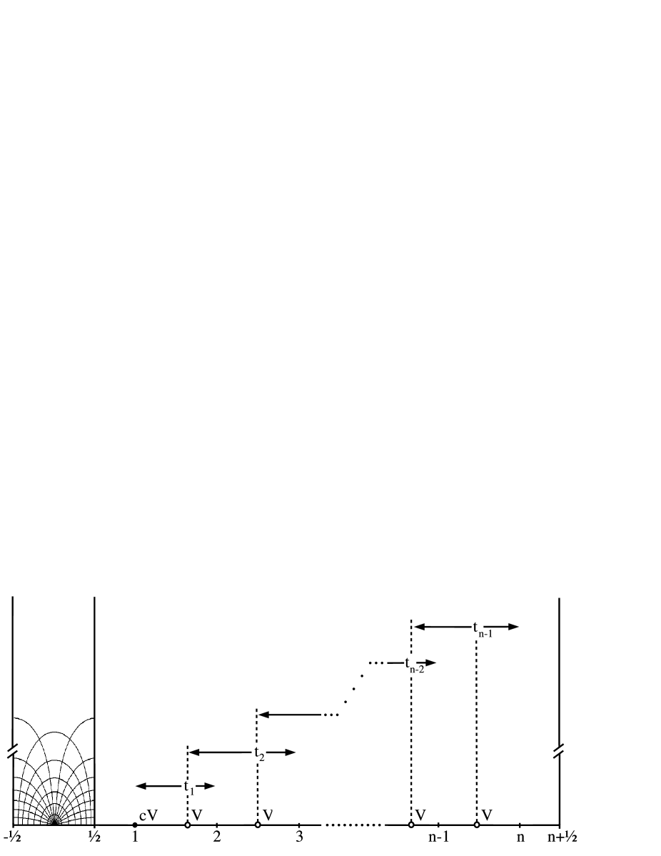
This form of $\Psi_{L}^{(3)}$ can be generalized to $\Psi_{L}^{(n)}$ for any $n$ as follows:

$$\begin{split}\langle\,\phi\,,\Psi_{L}^{(n)}\,\rangle&=\Bigl{\langle}\,f\circ\phi(0)\,\,cV(1)\int_{1}^{2}dt_{1}\int_{t_{1}}^{3}dt_{2}\int_{t_{2}}^{4}dt_{3}\,\ldots\,\int_{t_{n-2}}^{n}dt_{n-1}\,V(t_{1})\,V(t_{2})\,V(t_{3})\,\ldots\,V(t_{n-1})\Bigr{\rangle}_{{\cal W}_{n}}\\ &=\Bigl{\langle}\,f\circ\phi(0)\,\,cV(1)\prod_{j=1}^{n-1}\,\int_{t_{j-1}}^{j+1}dt_{j}\,V(t_{j})\,\Bigr{\rangle}_{{\cal W}_{n}}\qquad\text{ with}\quad t_{0}\equiv 1\,.\end{split}$$ (2.23)

See figure 7. It is straightforward to show that $\Psi_{L}^{(n)}$ satisfies the equation of motion:

Figure 7: Illustration of $\Psi_{L}^{(n)}$. The solid dot represents the $cV$ insertion, and the circles represent the $V$ insertions. The integration region of $t_{j}$ is from $t_{j-1}$ to $j+1$.

$$\begin{split}\langle\,\phi&\,,Q_{B}\Psi_{L}^{(n)}\,\rangle\\ =&-\sum_{i=1}^{n-1}\,\Bigl{\langle}\,f\circ\phi(0)\,cV(1)\prod_{j=1}^{i-1}\int_{t_{j-1}}^{j+1}dt_{j}V(t_{j})\,\int_{t_{i-1}}^{i+1}dt_{i}\,\partial_{t_{i}}\,[\,cV(t_{i})\,]\,\prod_{k=i+1}^{n-1}\int_{t_{k-1}}^{k+1}dt_{k}V(t_{k})\,\Bigr{\rangle}_{{\cal W}_{n}}\\ =&-\sum_{i=1}^{n-1}\,\Bigl{\langle}\,f\circ\phi(0)\,cV(1)\prod_{j=1}^{i-1}\int_{t_{j-1}}^{j+1}dt_{j}V(t_{j})\,\,cV(i+1)\,\int_{i+1}^{i+2}dt_{i+1}\ldots\int_{t_{n-2}}^{n}dt_{n-1}\,V(t_{i+1})\ldots V(t_{k})\,\Bigr{\rangle}_{{\cal W}_{n}}\\ &+\sum_{i=2}^{n-1}\,\Bigl{\langle}\,f\circ\phi(0)\,cV(1)\prod_{j=1}^{i-1}\int_{t_{j-1}}^{j+1}dt_{j}V(t_{j})\,\,cV(t_{i-1})\,\int_{t_{i-1}}^{i+2}dt_{i+1}\ldots\int_{t_{n-2}}^{n}dt_{n-1}\,V(t_{i+1})\ldots V(t_{k})\,\Bigr{\rangle}_{{\cal W}_{n}}\\ &+\sum_{i=1}^{n-2}\,\Bigl{\langle}\,f\circ\phi(0)\,cV(1)\prod_{j=1}^{i-1}\int_{t_{j-1}}^{j+1}dt_{j}V(t_{j})\,\int_{t_{i-1}}^{i+1}dt_{i}\,cV(t_{i})\,\partial_{t_{i}}\Biggl{[}\,\prod_{k=i+1}^{n-1}\int_{t_{k-1}}^{k+1}dt_{k}V(t_{k})\,\Biggr{]}\,\Bigr{\rangle}_{{\cal W}_{n}}\,.\end{split}$$ (2.24)

By carrying out the differentiation in the last line, we find that the last line precisely cancels the second line on the right-hand side. The remaining first line on the right-hand side is a sum of ${}-\Psi^{(i)}\ast\Psi^{(n-i)}$ over $i$. We have thus shown

$$\langle\,\phi\,,\,Q_{B}\Psi_{L}^{(n)}\,\rangle=-\sum_{i=1}^{n-1}\,\langle\,\phi\,,\Psi^{(i)}\ast\Psi^{(n-i)}\,\rangle\,.$$ (2.25)

It is convenient to introduce the following notation:

$$\begin{split}V_{L}^{(n)}(1,n+1)&\equiv\int_{1}^{2}dt_{1}\int_{t_{1}}^{3}dt_{2}\int_{t_{2}}^{4}dt_{3}\,\ldots\,\int_{t_{n-1}}^{n+1}dt_{n}\,V(t_{1})\,V(t_{2})\,\ldots\,V(t_{n})\quad\text{ for }\quad n\geq 1\,,\\ V_{L}^{(0)}(1,1)&\equiv 1\,.\end{split}$$ (2.26)

The superscript $(n)$ indicates the number of operators and $(1,n+1)$ indicates the region where operators are inserted, although this notation is slightly redundant because the number of operators and the length of the region are correlated for $V_{L}^{(n)}(1,n+1)$. The solution $\Psi_{L}^{(n)}$ can now be compactly written as

$$\langle\,\phi\,,\Psi_{L}^{(n)}\,\rangle=\langle\,f\circ\phi(0)\,\,cV(1)\,\,V_{L}^{(n-1)}(1,n)\,\rangle_{{\cal W}_{n}}\,.$$ (2.27)

The state $\Psi_{L}$ defined by

$$\Psi_{L}=\sum_{n=1}^{\infty}\lambda^{n}\,\Psi_{L}^{(n)}$$ (2.28)

thus solves the equation of motion to all orders in $\lambda$.

2.2 Solutions satisfying the reality condition

The solution $\Psi_{L}$ constructed in the previous subsection satisfies the equation of motion, but it does not satisfy the reality condition on the string field. In this subsection, we construct a solution satisfying the reality condition from $\Psi_{L}$.

2.2.1 The reality condition

The string field $\Psi$ must have a definite parity under the combination of the Hermitean conjugation (hc) and the inverse BPZ conjugation ($\text{bpz}^{-1}$) to guarantee that the string field theory action is real [43]. We define the conjugate $A^{\ddagger}$ of a string field $A$ by

$$A^{\ddagger}\equiv\text{bpz}^{-1}\circ\text{hc}\,(A)\,.$$ (2.29)

With this definition, the following relations hold:

$$(Q_{B}A)^{\ddagger} = {}-(-1)^{A}\,Q_{B}A^{\ddagger}\,,$$ (2.30)

$$(A\ast B)^{\ddagger} = B^{\ddagger}\ast A^{\ddagger}\,.$$ (2.31)

Here and in what follows a string field in the exponent of $(-1)$ denotes its Grassmann property: it is $0$ mod $2$ for a Grassmann-even state and $1$ mod $2$ for a Grassmann-odd state. Since the string field $\Psi$ is Grassmann odd, it must be even under the conjugation $\Psi^{\ddagger}=\Psi$ in order that $Q_{B}\Psi$ and $\Psi\ast\Psi$ have the same parity. We will say that a string field of ghost number one is real when it is even under the conjugation.

The class of states we use in constructing solutions for marginal deformations are made of wedge states with insertions of $cV$ and $V$. Let us consider the conjugate of a state in this class. The wedge state $W_{\alpha}$ [44] is even under the conjugation $W_{\alpha}^{\ddagger}=W_{\alpha}$ because it is constructed from the $SL(2,R)$-invariant vacuum $|0\rangle$ satisfying $|0\rangle^{\ddagger}=|0\rangle$ by acting with BPZ-even Virasoro generators $L_{-2},\,L_{-4},\,\ldots\,$. The first term $\Psi^{(1)}$ in the solution must be even $(\Psi^{(1)})^{\ddagger}=\Psi^{(1)}$, as we discussed above. Therefore, the conjugate of $W_{\alpha}\ast\Psi^{(1)}\ast W_{\beta}$ is $W_{\beta}\ast\Psi^{(1)}\ast W_{\alpha}$. This means that the operator $cV(t)$ on ${\cal W}_{n}$ is mapped to $cV(n+1-t)$ under the conjugation:

$$cV(t)~{}\longrightarrow~{}cV(n+1-t)\quad\text{on}\quad{\cal W}_{n}\,.$$ (2.32)

Its derivative $\partial_{t}\,[\,cV(t)\,]$ at $t=a$ is then mapped to ${}-\partial_{t}\,[\,cV(t)\,]$ at $t=n+1-a$. Since $\partial_{t}\,[\,cV(t)\,]$ is the BRST transformation of $V(t)$, this means that $Q_{B}\cdot V(a)$ is mapped to ${}-Q_{B}\cdot V(n+1-a)$ on ${\cal W}_{n}$. It then follows from (2.30) that $V(t)$ is mapped under the conjugation as follows:

$$V(t)~{}\longrightarrow~{}V(n+1-t)\quad\text{on}\quad{\cal W}_{n}\,.$$ (2.33)

It is straightforward to generalize the argument to the case with multiple operator insertions. The conjugate of the state made of the wedge state $W_{n}$ with $cV(t_{1}),V(t_{2}),V(t_{3}),\ldots,V(t_{m})$ is therefore the state made of $W_{n}$ with $V(n+1-t_{m}),V(n+1-t_{m-1}),\ldots,V(n+1-t_{2}),cV(n+1-t_{1})$.

The state $\Psi_{L}^{(n)}$ with $n\geq 2$ does not satisfy the reality condition. Indeed, the operator $V_{L}^{(n-1)}(1,n)$ defined in (2.26) is mapped as

$$\begin{split}\int_{1}^{2}dt_{1}\int_{t_{1}}^{3}dt_{2}&\int_{t_{2}}^{4}dt_{3}\,\ldots\,\int_{t_{n-2}}^{n}dt_{n-1}\,V(t_{1})\,V(t_{2})\,\ldots\,V(t_{n-1})\\ ~{}\longrightarrow~{}&\int_{1}^{2}dt_{1}\int_{t_{1}}^{3}dt_{2}\int_{t_{2}}^{4}dt_{3}\,\ldots\,\int_{t_{n-2}}^{n}dt_{n-1}\,V(n+1-t_{n-1})\,V(n+1-t_{n-2})\,\ldots\,V(n+1-t_{1})\\ &=\int_{n-1}^{n}dt^{\prime}_{1}\int_{n-2}^{t^{\prime}_{1}}dt^{\prime}_{2}\int_{n-3}^{t^{\prime}_{2}}dt^{\prime}_{3}\ldots\int_{1}^{t^{\prime}_{n-2}}dt^{\prime}_{n-1}\,V(t^{\prime}_{n-1})\,V(t^{\prime}_{n-2})\ldots V(t^{\prime}_{1})\end{split}$$ (2.34)

under the conjugation, where $t^{\prime}_{i}=n+1-t_{i}$. We denote the conjugate of $\Psi_{L}^{(n)}$ by $\Psi_{R}^{(n)}$. It is given by

$$\langle\,\phi\,,\Psi_{R}^{(n)}\,\rangle=\langle\,\phi\,,(\Psi_{L}^{(n)})^{\ddagger}\,\rangle=\langle\,f\circ\phi(0)\,\,\,V_{R}^{(n-1)}(1,n)\,\,cV(n)\,\rangle_{{\cal W}_{n}}\,,$$ (2.35)

where we defined

$$\begin{split}V_{R}^{(n)}(1,n+1)&\equiv\int_{n}^{n+1}dt_{1}\int_{n-1}^{t_{1}}dt_{2}\int_{n-2}^{t_{2}}dt_{3}\ldots\int_{1}^{t_{n-1}}dt_{n}\,V(t_{n})\,V(t_{n-1})\ldots V(t_{1})\quad\text{ for }\quad n\geq 1\,,\\ V_{R}^{(0)}(1,1)&\equiv 1\,.\end{split}$$ (2.36)

If $\Psi$ satisfies the equation of motion, its conjugate $\Psi^{\ddagger}$ also satisfies the equation of motion because

$$Q_{B}\Psi^{\ddagger}+\Psi^{\ddagger}\ast\Psi^{\ddagger}=(Q_{B}\Psi+\Psi\ast\Psi)^{\ddagger}=0\,.$$ (2.37)

Therefore, $\Psi_{R}$ defined by

$$\Psi_{R}=\sum_{n=1}^{\infty}\lambda^{n}\,\Psi_{R}^{(n)}$$ (2.38)

satisfies the equation of motion.

2.2.2 Gauge transformation

We have found two solutions $\Psi_{L}$ and $\Psi_{R}$, and we expect that they are related by a gauge transformation generated by some gauge parameter $U$:

$$\Psi_{R}\,=\,U^{-1}\ast\Psi_{L}\ast U+U^{-1}\ast Q_{B}U\,.$$ (2.39)

For a physical gauge transformation which relates two string fields satisfying the reality condition, the gauge parameter $U$ must satisfy the unitarity relation $U^{\ddagger}=U^{-1}$. As we will see later, the gauge parameter $U$ that relates $\Psi_{L}$ and $\Psi_{R}$ is even under the conjugation: $U^{\ddagger}=U$. The component fields of $\Psi_{L}$ and $\Psi_{R}$ which do not satisfy the reality condition are thus related through the component fields of $U$ which also violate the reality condition on the gauge parameter.

Let us now construct $U$ which relates $\Psi_{L}$ and $\Psi_{R}$. It is convenient to rewrite the equation (2.39) as follows:

$$Q_{B}U\,=\,U\ast\Psi_{R}\,-\,\Psi_{L}\ast U\,.$$ (2.40)

We can expand $U$ as

$$U=\sum_{n=0}^{\infty}\lambda^{n}\,U^{(n)}\quad\text{with}\quad U^{(0)}=1\,,$$ (2.41)

and we solve the equation perturbatively in $\lambda$. We can choose

$$U^{(1)}=0$$ (2.42)

because $\Psi_{L}^{(1)}=\Psi_{R}^{(1)}$ and therefore $Q_{B}U^{(1)}=0$. The equation for $U^{(2)}$ is

$$\langle\,\phi,Q_{B}\,U^{(2)}\,\rangle=\langle\,\phi,\Psi_{R}^{(2)}\,\rangle-\langle\,\phi,\Psi_{L}^{(2)}\,\rangle=\langle\,f\circ\phi(0)\,[\,V(1,2)\,cV(2)-cV(1)\,V(1,2)\,]\,\rangle_{{\cal W}_{2}}\,.$$ (2.43)

This can be easily solved using the formula (2.16), and a solution is

$$\langle\,\phi,U^{(2)}\,\rangle=\frac{1}{2}\,\langle\,f\circ\phi(0)\,\left(V(1,2)\right)^{2}\,\rangle_{{\cal W}_{2}}\,.$$ (2.44)

We can construct $U^{(n)}$ at higher orders recursively in this way. However, we can infer $U^{(n)}$ from the structure of (2.40). If we assume that $U$ can be written without using $c$ ghosts, the only $c$ ghost is inserted at $t=n$ in the $\mathcal{O}(\lambda^{n})$ term of $\langle\,\phi,U\ast\Psi_{R}\,\rangle$ when represented on ${\cal W}_{n}$ and at $t=1$ on ${\cal W}_{n}$ in the $\mathcal{O}(\lambda^{n})$ term of $\langle\,\phi,\Psi_{L}\ast U\,\rangle$. This motivates us to make the following ansatz:

$$\langle\,\phi,U^{(n)}\,\rangle\propto\langle\,f\circ\phi(0)\,V^{(n)}(1,n)\,\rangle_{{\cal W}_{n}}\,,$$ (2.45)

where

$$V^{(n)}(a,b)\equiv\frac{1}{n!}\left(V(a,b)\right)^{n}\quad\text{ for }\quad n\geq 1\,,\qquad V^{(0)}(a,b)\equiv 1\,.$$ (2.46)

We in fact show that the gauge transformation $U$ in (2.39) is given by

$1+\frac{\lambda^{2}}{2!}$ $\,+\,\,\frac{\lambda^{3}}{3!}$ $+\,\,\ldots$

Figure 8: Illustration of the expansion $U=1+\lambda^{2}\,U^{(2)}+\lambda^{3}\,U^{(3)}+\mathcal{O}(\lambda^{4})$.

$$\langle\,\phi\,,U^{(n)}\,\rangle=\langle\,f\circ\phi(0)\,\,V^{(n)}(1,n)\,\rangle_{{\cal W}_{n}}\,.$$ (2.47)

See figure 8. The BRST transformation of $U^{(n)}$ given in (2.47) is

$$\langle\,\phi,Q_{B}U^{(n)}\,\rangle=\bigl{\langle}\,f\circ\phi(0)\,\,\,\bigl{(}V^{(n-1)}(1,n)\,cV(n)\,-\,cV(1)\,V^{(n-1)}(1,n)\bigr{)}\,\bigr{\rangle}_{{\cal W}_{n}}\,,$$ (2.48)

where we used (2.16). For the special case of $n=1$, the terms on the right-hand side cancel, which is consistent because $U^{(1)}=0$. The $\mathcal{O}(\lambda^{n})$ term of $U\ast\Psi_{R}\,-\,\Psi_{L}\ast U$ in (2.40) is given by

$$\begin{split}&\sum_{m=1}^{n}\langle\,f\circ\phi(0)\,\,\,V^{(n-m)}(1,n-m)\,V_{R}^{(m-1)}(n-m+1,n)\,cV(n)\,\rangle_{{\cal W}_{n}}\\ &-\sum_{m=1}^{n}\langle\,f\circ\phi(0)\,\,\,cV(1)\,V_{L}^{(m-1)}(1,m)\,V^{(n-m)}(m+1,n)\,\rangle_{{\cal W}_{n}}\,.\end{split}$$ (2.49)

The proof of (2.40) for $U$ given in (2.47) thus reduces to showing that

$$\langle\,f\circ\phi(0)\,\,\,cV(1)\,V^{(n-1)}(1,n)\,\rangle_{{\cal W}_{n}}\,=\sum_{m=1}^{n}\langle\,f\circ\phi(0)\,\,\,cV(1)\,V_{L}^{(m-1)}(1,m)\,V^{(n-m)}(m+1,n)\,\rangle_{{\cal W}_{n}}\,$$ (2.50)

and

$$\langle\,f\circ\phi(0)\,\,\,V^{(n-1)}(1,n)\,cV(n)\,\rangle_{{\cal W}_{n}}\,=\sum_{m=1}^{n}\langle\,f\circ\phi(0)\,\,\,V^{(n-m)}(1,n-m)\,V_{R}^{(m-1)}(n-m+1,n)\,cV(n)\,\rangle_{{\cal W}_{n}}\,.$$ (2.51)

Since the second equation follows from the first one by the conjugation, it is sufficient to show (2.50). The operator $V^{(n-1)}(1,n)$ on the left-hand side can be written in a path-ordered form as follows:

$$V^{(n-1)}(1,n)=\int_{1}^{n}dt_{1}\int_{t_{1}}^{n}dt_{2}\ldots\int_{t_{n-2}}^{n}dt_{n-1}\,V(t_{1})\ldots V(t_{n-1})\,.$$ (2.52)

We now decompose the integration region $1\leq t_{1}\leq t_{2}\leq\ldots\leq t_{n-1}\leq n$ in the following way:

$$\begin{split}&t_{1}\geq 2\,,\\ &t_{1}\leq 2\,,\,t_{2}\geq 3\,,\\ &t_{1}\leq 2\,,\,t_{2}\leq 3\,,\,t_{3}\geq 4\,,\\ &\qquad\qquad\vdots\\ &t_{1}\leq 2\,,\,t_{2}\leq 3\,,\,\ldots\,,\,t_{m-1}\leq m\,,\,t_{m}\geq m+1\,,\\ &\qquad\qquad\vdots\\ &t_{1}\leq 2\,,\,t_{2}\leq 3\,,\,t_{3}\leq 4\,,\,\ldots\ldots\ldots\,,\,t_{n-2}\leq n-1\,,\,t_{n-1}\geq n\,,\\ &t_{1}\leq 2\,,\,t_{2}\leq 3\,,\,t_{3}\leq 4\,,\,\ldots\ldots\ldots\,,\,t_{n-2}\leq n-1\,,\,t_{n-1}\leq n\,.\end{split}$$ (2.53)

This decomposition of the integration region precisely matches the right-hand side of (2.50). For example, the fourth line of (2.53) corresponds to the integration region for the product of the operators $V_{L}^{(m-1)}(1,m)\,V^{(n-m)}(m+1,n)$. Furthermore, the fifth line vanishes because of the vanishing integration range $n\leq t_{n-1}\leq n$. This is consistent with the right-hand side of (2.50) because $V^{(1)}(n,n)=0$. The last line is nonvanishing and corresponds to $V_{L}^{(n-1)}(1,n)\,V^{(0)}(n+1,n)=V_{L}^{(n-1)}(1,n)$, where we used $V^{(0)}(a,b)\equiv 1$. We conclude that

$$V^{(n-1)}(1,n)\,=\,\sum_{m=1}^{n}\,V_{L}^{(m-1)}(1,m)\,V^{(n-m)}(m+1,n)\,,$$ (2.54)

and we have thus shown (2.50). This completes the proof that $U$ is the gauge transformation that relates $\Psi_{L}$ and $\Psi_{R}$.

2.2.3 Construction of a real solution

The state $U$ takes the form

$$U=1+\sum_{n=2}^{\infty}\lambda^{n}\,U^{(n)}\,,$$ (2.55)

and $U^{(n)}$ is even under the conjugation: $(U^{(n)})^{\ddagger}=U^{(n)}$. If a state $X$ is even under the conjugation, then $\ln(1+X)$ defined by

$$\ln(1+X)\equiv\sum_{n=1}^{\infty}\frac{(-1)^{n+1}}{n}\,\underbrace{\,X\ast X\ast\ldots\ast X\,}_{n}$$ (2.56)

is also even. If a state $Y$ is even, then $\exp\,(a\,Y)$ with real $a$ defined by

$$\exp\,(a\,Y)\equiv 1+\sum_{n=1}^{\infty}\frac{a^{n}}{n!}\,\underbrace{\,Y\ast Y\ast\ldots\ast Y\,}_{n}$$ (2.57)

is also even. Therefore, $(1+X)^{-1}$, $\sqrt{1+X}$ and $1/\sqrt{1+X}$ defined by

$$\begin{split}(1+X)^{-1}&\equiv\exp\left[\,-\ln(1+X)\,\right]=1+\sum_{n=1}^{\infty}\,(-1)^{n}\,\underbrace{\,X\ast X\ast\ldots\ast X\,}_{n}\,,\\ \sqrt{1+X}&\equiv\exp\left[\,\frac{1}{2}\,\ln(1+X)\,\right]\,,\qquad\frac{1}{\sqrt{1+X}}\equiv\exp\left[\,-\frac{1}{2}\,\ln(1+X)\,\right]\end{split}$$ (2.58)

are all even if $X^{\ddagger}=X$. We define $U^{-1}$, $\sqrt{U}$, and $1/\sqrt{U}$ in this way, which are well defined to all orders in $\lambda$ and are even under the conjugation.

We can now construct a real solution $\Psi$ from $\Psi_{L}$ as follows:

$$\begin{split}\Psi&\equiv\frac{1}{\sqrt{U}}\ast\Psi_{L}\ast\sqrt{U}+\frac{1}{\sqrt{U}}\ast Q_{B}\,\sqrt{U}\\ &=\sqrt{U}\ast\Psi_{R}\ast\frac{1}{\sqrt{U}}+\sqrt{U}\ast Q_{B}\,\frac{1}{\sqrt{U}}\\ &=\frac{1}{2}\,\biggl{[}\,\frac{1}{\sqrt{U}}\ast\Psi_{L}\ast\sqrt{U}+\sqrt{U}\ast\Psi_{R}\ast\frac{1}{\sqrt{U}}+\frac{1}{\sqrt{U}}\ast Q_{B}\,\sqrt{U}-Q_{B}\,\sqrt{U}\ast\frac{1}{\sqrt{U}}\,\biggr{]}\,.\end{split}$$ (2.59)

The second expression is obtained from the first one using $Q_{B}U=U\ast\Psi_{R}-\Psi_{L}\ast U$, and $\Psi$ manifestly satisfies the reality condition in the third expression because of the relations $\Psi_{L}^{\ddagger}=\Psi_{R}$, $(\sqrt{U}\,)^{\ddagger}=\sqrt{U}$, $(1/\sqrt{U}\,)^{\ddagger}=1/\sqrt{U}$, and $(Q_{B}\,\sqrt{U}\,)^{\ddagger}={}-Q_{B}\,\sqrt{U}$. The state $\Psi$ also satisfies the equation of motion because it is obtained from the solution $\Psi_{L}$ by the gauge transformation generated by $\sqrt{U}$.

We have successfully constructed real analytic solutions for marginal deformations with regular operator products. To summarize, our solution takes the form

$$\Psi=\frac{1}{\sqrt{U}}\ast\Psi_{L}\ast\sqrt{U}+\frac{1}{\sqrt{U}}\ast Q_{B}\,\sqrt{U}\,,$$ (2.60)

where $\Psi_{L}$ and $U$ are defined by

$$\begin{split}\Psi_{L}&=\sum_{n=1}^{\infty}\lambda^{n}\,\Psi^{(n)}_{L}\,,\\ \langle\,\phi\,,\Psi^{(n)}_{L}\,\rangle&=\,\langle\,f\circ\phi(0)\,\,cV(1)\,\,V_{L}^{(n-1)}(1,n)\,\rangle_{{\cal W}_{n}}\,\\ &=\int_{1}^{2}dt_{1}\int_{t_{1}}^{3}dt_{2}\,\ldots\,\int_{t_{n-2}}^{n}dt_{n-1}\,\langle\,f\circ\phi(0)\,\,cV(1)\,\,V(t_{1})\,V(t_{2})\,\ldots\,V(t_{n-1})\,\rangle_{{\cal W}_{n}}\,,\\ U&=1+\sum_{n=2}^{\infty}\lambda^{n}\,U^{(n)}\,,\\ \langle\,\phi\,,U^{(n)}\,\rangle&=\langle\,f\circ\phi(0)\,V^{(n)}(1,n)\,\rangle_{{\cal W}_{n}}\,\\ &=\frac{1}{n!}\int_{1}^{n}dt_{1}\int_{1}^{n}dt_{2}\ldots\int_{1}^{n}dt_{n}\,\langle\,f\circ\phi(0)\,V(t_{1})\,V(t_{2})\,\ldots V(t_{n})\,\rangle_{{\cal W}_{n}}\,.\end{split}$$ (2.61)

2.3 Generalization of wedge states

In the previous subsection, we found the identity (2.54). It is simply a consequence of the decomposition of the integral region (2.53). The identity (2.54) can be generalized in the following way. We define $V_{L,\alpha}^{(n)}(1,n+\alpha)$ for $\alpha\geq 0$ by

$$\begin{split}V_{L,\alpha}^{(n)}(1,n+\alpha)&\equiv\int_{1}^{1+\alpha}dt_{1}\int_{t_{1}}^{2+\alpha}dt_{2}\int_{t_{2}}^{3+\alpha}dt_{3}\,\ldots\,\int_{t_{n-1}}^{n+\alpha}dt_{n}\,V(t_{1})\,V(t_{2})\,\ldots\,V(t_{n})\quad\text{ for }\quad n\geq 1\,,\\ V_{L,\alpha}^{(0)}(1,\alpha)&\equiv 1\,.\end{split}$$ (2.62)

This reduces to $V_{L}^{(n)}(1,n+1)$ defined in (2.26) when $\alpha=1$. We then find that

$$V^{(n)}(1,n+\alpha+\beta)\,=\,\sum_{m=0}^{n}V^{(m)}_{L,\alpha}(1,m+\alpha)\,V^{(n-m)}(m+\alpha+1,n+\alpha+\beta)$$ (2.63)

for any non-negative real numbers $\alpha$ and $\beta$. This identity reduces to (2.54) when $\alpha=1$, $\beta=0$. This generalized identity can be shown, as before, by decomposing the path-ordered integration region $1\leq t_{1}\leq t_{2}\leq\ldots\leq t_{n}\leq n+\alpha+\beta$ of $V^{(n)}(1,n+\alpha+\beta)$ in the following way:

$$\begin{split}&t_{1}\geq 1+\alpha\,,\\ &t_{1}\leq 1+\alpha\,,\,t_{2}\geq 2+\alpha\,,\\ &t_{1}\leq 1+\alpha\,,\,t_{2}\leq 2+\alpha\,,\,t_{3}\geq 3+\alpha\,,\\ &\qquad\qquad\vdots\\ &t_{1}\leq 1+\alpha\,,\,t_{2}\leq 2+\alpha\,,\,\ldots\,,\,t_{m}\leq m+\alpha\,,\,t_{m+1}\geq m+1+\alpha\,,\\ &\qquad\qquad\vdots\\ &t_{1}\leq 1+\alpha\,,\,t_{2}\leq 2+\alpha\,,\,t_{3}\leq 3+\alpha\,,\,\ldots\ldots\ldots\,,\,t_{n-1}\leq n-1+\alpha\,,\,t_{n}\geq n+\alpha\,,\\ &t_{1}\leq 1+\alpha\,,\,t_{2}\leq 2+\alpha\,,\,t_{3}\leq 3+\alpha\,,\,\ldots\ldots\ldots\,,\,t_{n-1}\leq n-1+\alpha\,,\,t_{n}\leq n+\alpha\,.\end{split}$$ (2.64)

This identity can be promoted to a relation of string fields. We define $U_{\alpha}$ and $U_{L,\alpha}$ with $\alpha\geq 0$ by

$$\begin{split}U_{\alpha}\equiv\sum_{n=0}^{\infty}\,\lambda^{n}\,U_{\alpha}^{(n)}\,,\qquad U_{L,\alpha}\equiv\sum_{n=0}^{\infty}\,\lambda^{n}\,U_{L,\alpha}^{(n)}\,,\end{split}$$ (2.65)

where

$$\begin{split}\langle\,\phi\,,U_{\alpha}^{(n)}\,\rangle&=\langle\,f\circ\phi(0)\,\,\,V^{(n)}(1,n+\alpha)\,\rangle_{{\cal W}_{n+\alpha}}\quad\text{for}\quad n+\alpha>0\,,\quad U_{0}^{(0)}=1\,,\\ \langle\,\phi\,,U_{L,\alpha}^{(n)}\,\rangle&=\langle\,f\circ\phi(0)\,\,\,V_{L,\alpha}^{(n)}(1,n+\alpha)\,\rangle_{{\cal W}_{n+\alpha}}\quad\text{for}\quad n+\alpha>0\,,\quad U_{L,0}^{(0)}=1\,.\end{split}$$ (2.66)

The gauge parameter $U$ in the previous subsection is thus

$$U=U_{0}\,,$$ (2.67)

and the solution $\Psi_{L}$ in (2.27) is $U_{L,1}$ with an extra insertion of $\lambda\,cV(1)$. It then follows from (2.63) that

$$U_{\alpha+\beta}=U_{L,\alpha}\ast U_{\beta}\,.$$ (2.68)

When $\beta=0$, we have

$$U_{\alpha}=U_{L,\alpha}\ast U\,,$$ (2.69)

where we have used $U_{0}=U$. As we discussed in the previous subsection, the inverse of $U$ is well defined to all orders in $\lambda$. We thus find that

$$U_{L,\alpha}=U_{\alpha}\ast U^{-1}\,.$$ (2.70)

It follows from this and (2.68) that

$$U_{\alpha+\beta}=U_{\alpha}\ast U^{-1}\ast U_{\beta}\,.$$ (2.71)

The state $U_{\alpha}$ is $W_{\alpha}+\mathcal{O}(\lambda)$ for $\alpha>0$, where $W_{\alpha}$ is the well-known wedge state defined by

$$\langle\,\phi\,,W_{\alpha}\,\rangle=\langle\,f\circ\phi(0)\,\rangle_{{\cal W}_{\alpha}}\,.$$ (2.72)

The relation (2.71) for positive $\alpha$ and $\beta$ thus reduces to the famous relation $W_{\alpha+\beta}=W_{\alpha}\ast W_{\beta}$ when $\lambda=0$, and the state $U_{\alpha}$ can be thought of as a generalization of the wedge state $W_{\alpha}$. When $\alpha$ is a positive integer, $U_{\alpha}$ can be written in terms of $U_{1}$ and $U^{-1}$:

$$\begin{split}&U_{2}=U_{1}\ast U^{-1}\ast U_{1}\,,\\ &U_{3}=U_{1}\ast U^{-1}\ast U_{1}\ast U^{-1}\ast U_{1}\,,\\ &U_{4}=U_{1}\ast U^{-1}\ast U_{1}\ast U^{-1}\ast U_{1}\ast U^{-1}\ast U_{1}\,,\\ &\qquad\qquad\vdots\\ \end{split}$$ (2.73)

This structure indicates a modification of the star product for finite $\lambda$ defined by

$$A\star B\equiv A\ast U^{-1}\ast B\,,$$ (2.74)

and the relation (2.71) can be written as

$$U_{\alpha+\beta}=U_{\alpha}\star U_{\beta}\,.$$ (2.75)

On a technical level, the relation (2.71) will play an important role in the next section for the construction of solutions associated with general marginal deformations. On a more conceptual level, we will see in section 5 that the modified star product (2.74) naturally appears in the string field theory action expanded around a deformed background.

3 Marginal deformations with singular operator products

3.1 Another form of the solution with regular operator products

In the process of constructing a real solution from $\Psi_{L}$ in the previous section, we proved that

$$Q_{B}\,U=U\ast\Psi_{R}-\Psi_{L}\ast U\,.$$ (3.1)

As we have seen in (2.48), the BRST transformation of $U$ can be decomposed into two pieces:

$$Q_{B}\,U=A_{R}-A_{L}\,,$$ (3.2)

where $A_{L}$ and $A_{R}$ are given by

$\lambda$ $+\,\,\lambda^{2}$ $+\,\,\frac{\lambda^{3}}{2}$ $+\,\ldots$

Figure 9: Illustration of the expansion $A_{L}=\lambda\,A_{L}^{(1)}+\lambda^{2}\,A_{L}^{(2)}+\lambda^{3}\,A_{L}^{(3)}+\mathcal{O}(\lambda^{4})$.

$$\begin{split}\langle\,\phi\,,A_{L}\,\rangle&=\sum_{n=1}^{\infty}\lambda^{n}\,\langle\,f\circ\phi(0)\,cV(1)\,V^{(n-1)}(1,n)\,\rangle_{{\cal W}_{n}}\,,\\ \langle\,\phi\,,A_{R}\,\rangle&=\sum_{n=1}^{\infty}\lambda^{n}\,\langle\,f\circ\phi(0)\,V^{(n-1)}(1,n)\,cV(n)\,\rangle_{{\cal W}_{n}}\,.\end{split}$$ (3.3)

See figure 9. At $\mathcal{O}(\lambda^{n})$ with $n\geq 2$, $A_{L}$ and $A_{R}$ account for the term with $cV(1)$ and the term with $cV(n)$ in $Q_{B}U^{(n)}$, respectively. At $\mathcal{O}(\lambda)$, $Q_{B}\,U$ vanishes because $U^{(1)}=0$, but we have chosen $A_{L}$ and $A_{R}$ at $\mathcal{O}(\lambda)$ to be $\lambda\,\Psi^{(1)}$ for later convenience.

In the proof of (3.1), we have actually shown that

$$A_{L}=\Psi_{L}\ast U\,,\qquad A_{R}=U\ast\Psi_{R}\,.$$ (3.4)

As we discussed in the previous section, the inverse of $U$ is well defined to all orders in $\lambda$. We thus obtain new expressions for $\Psi_{L}$ and $\Psi_{R}$:

$$\Psi_{L}=A_{L}\ast U^{-1}\,,\qquad\Psi_{R}=U^{-1}\ast A_{R}\,.$$ (3.5)

We have shown that $\Psi_{L}$ with $\Psi_{L}^{(n)}$ in the form of (2.27) satisfies the equation of motion. Let us now see how $\Psi_{L}$ in the new form satisfies the equation of motion. The BRST transformation of $\Psi_{L}$ can be calculated as follows:

$$\begin{split}Q_{B}\Psi_{L}\,&=\,Q_{B}\,(A_{L}\ast U^{-1})\\ &=(Q_{B}A_{L})\ast U^{-1}+A_{L}\ast U^{-1}\ast(Q_{B}U)\ast U^{-1}\\ &=(Q_{B}A_{L})\ast U^{-1}+A_{L}\ast U^{-1}\ast(A_{R}-A_{L})\ast U^{-1}\\ &=(Q_{B}A_{L}+A_{L}\ast U^{-1}\ast A_{R})\ast U^{-1}-A_{L}\ast U^{-1}\ast A_{L}\ast U^{-1}\\ &=(Q_{B}A_{L}+A_{L}\ast U^{-1}\ast A_{R})\ast U^{-1}-\Psi_{L}\ast\Psi_{L}\,.\end{split}$$ (3.6)

Therefore, the equation of motion is satisfied if

$${}-Q_{B}A_{L}=A_{L}\ast U^{-1}\ast A_{R}\,.$$ (3.7)

The left-hand side of the equation can be calculated as follows:

$${}-\langle\,\phi\,,Q_{B}A_{L}\,\rangle=\sum_{n=2}^{\infty}\lambda^{n}\,\langle\,f\circ\phi(0)\,cV(1)\,V^{(n-2)}(1,n)\,cV(n)\,\rangle_{{\cal W}_{n}}\,.$$ (3.8)

Let us next consider the structure of the state $A_{L}\ast U^{-1}\ast A_{R}$ on the right-hand side of (3.7). The $\mathcal{O}(\lambda^{n})$ terms of $A_{L}$ and $A_{R}$ are made of the wedge state $W_{n}$ with operator insertions. The inverse $U^{-1}$ can be written as a linear combination of string products made of $\lambda^{n}\,U^{(n)}$, and their $\mathcal{O}(\lambda^{n})$ terms are again made of the wedge state $W_{n}$ with operator insertions. It thus follows that all of the $\mathcal{O}(\lambda^{n})$ terms of $A_{L}\ast U^{-1}\ast A_{R}$ are made of $W_{n}$ with operator insertions. This is consistent with the structure of (3.8). Furthermore, the insertions of $\lambda\,cV$ on the surface ${\cal W}_{n}$ are always $\lambda\,cV(1)$ and $\lambda\,cV(n)$, which is again consistent with the structure of (3.8). Finally, let us consider the structure of integrated vertex operators. The state ${}-Q_{B}A_{L}$ takes the form of the state $U_{2}$ defined in (2.65) with insertions of $\lambda\,cV$. Similarly, $A_{L}$ and $A_{R}$ take the form of $U_{1}$ with an insertion of $\lambda\,cV$. The equation (3.7) thus follows from (2.71) with $\alpha=\beta=1$:

$$U_{2}=U_{1}\ast U^{-1}\ast U_{1}\,.$$ (3.9)

We conclude that $\Psi_{L}$ of the form given in (3.5) satisfies the equation of motion.

3.2 Generalization to the case with singular operator products

The form $\Psi_{L}=A_{L}\ast U^{-1}$ for the solution can be generalized to the case where operator products of the marginal operator are singular. As we discussed in the introduction, let us denote the properly renormalized operator implementing the change of the boundary condition between the points $a$ and $b$ by $[\,e^{\lambda\,V(a,b)}\,]_{r}$, which is given in the form of an expansion in $\lambda$:

$$[\,e^{\lambda\,V(a,b)}\,]_{r}=\sum_{n=0}^{\infty}\,\frac{\lambda^{n}}{n!}\,[\,\left(V(a,b)\right)^{n}\,]_{r}\,,=\sum_{n=0}^{\infty}\lambda^{n}\,[\,V^{(n)}(a,b)\,]_{r}\,.$$ (3.10)

We define $U$ in the general case by

$$U\equiv\sum_{n=0}^{\infty}\,\lambda^{n}\,U^{(n)}\,,$$ (3.11)

where

$$\langle\,\phi\,,U^{(n)}\,\rangle=\langle\,f\circ\phi(0)\,\,[\,V^{(n)}(1,n)\,]_{r}\,\rangle_{{\cal W}_{n}}\,.$$ (3.12)

As we discussed in the introduction, we assume that the BRST transformation of $[\,e^{\lambda\,V(a,b)}\,]_{r}$ for any exactly marginal deformation takes the form

$$Q_{B}\cdot[\,e^{\lambda\,V(a,b)}\,]_{r}=[\,e^{\lambda\,V(a,b)}\,O_{R}(b)\,]_{r}-[\,O_{L}(a)\,e^{\lambda\,V(a,b)}\,]_{r}\,,$$ (3.13)

where $O_{L}$ and $O_{R}$ are $\lambda$-dependent, Grassmann-odd local operators. The operators $O_{L}$ and $O_{R}$ are closely related and mapped to each other under the conjugation discussed in § 2.2.1 when the reflection assumption (VI) is satisfied. We will discuss the relation between $O_{L}$ and $O_{R}$ in more detail in § 3.4, but it is relevant only when generating a real solution from $\Psi_{L}$ and we do not need to assume any relation between $O_{L}$ and $O_{R}$ in the construction of the solution $\Psi_{L}$. In the case of marginal deformations with regular operator products, we see from (2.16) that

$$Q_{B}\cdot e^{\lambda\,V(a,b)}=\lambda\,\bigl{[}\,e^{\lambda\,V(a,b)}\,cV(b)-cV(a)\,e^{\lambda\,V(a,b)}\,\Bigr{]}$$ (3.14)

and identify

$$O^{regular}_{L}=O^{regular}_{R}=\lambda\,cV\,.$$ (3.15)

In the case of marginal deformations with singular operator products, there can be corrections to $O_{L}$ and $O_{R}$, which are determined from the BRST transformation of $[\,V^{(n)}(a,b)\,]_{r}$ in the form

$$Q_{B}\cdot[\,V^{(n)}(a,b)\,]_{r}=\sum_{r=1}^{n}\,[\,V^{(n-r)}(a,b)\,O_{R}^{(r)}(b)\,]_{r}{}-\sum_{l=1}^{n}\,[\,O_{L}^{(l)}(a)\,V^{(n-l)}(a,b)\,]_{r}\,,$$ (3.16)

where $O_{L}$ and $O_{R}$ are expanded as follows:

$$O_{L}=\sum_{n=1}^{\infty}\,\lambda^{n}\,O_{L}^{(n)}\,,\qquad O_{R}=\sum_{n=1}^{\infty}\,\lambda^{n}\,O_{R}^{(n)}\,.$$ (3.17)

The operators $O_{L}^{(1)}$ and $O_{R}^{(1)}$ are determined from the BRST transformation of $[\,V^{(1)}(a,b)\,]_{r}$. Since $[\,V^{(1)}(a,b)\,]_{r}$ does not require any renormalization, we find

$$Q_{B}\cdot[\,V^{(1)}(a,b)\,]_{r}=Q_{B}\cdot V(a,b)=cV(b)-cV(a)$$ (3.18)

for any dimension-one primary field $V$. Thus the operators $O_{L}^{(1)}$ and $O_{R}^{(1)}$ are determined to be

$$O_{L}^{(1)}=O_{R}^{(1)}=cV$$ (3.19)

for any marginal deformation. Similarly, the operators $O_{L}^{(n)}$ and $O_{R}^{(n)}$ with $n\geq 2$ are determined from the BRST transformation of $[\,V^{(n)}(a,b)\,]_{r}$ with $n\geq 2$ , but we do not need any specific information on these operator in the construction of solutions. The BRST transformation of $U$ is then given by

$$Q_{B}\,U=A_{R}-A_{L}\,,$$ (3.20)

where

$$A_{L}\equiv\sum_{n=1}^{\infty}\,\lambda^{n}\,A_{L}^{(n)}\,,\qquad A_{R}\equiv\sum_{n=1}^{\infty}\,\lambda^{n}\,A_{R}^{(n)}\,,$$ (3.21)

with

$\frac{1}{2}$ $+$ $+$

Figure 10: Illustration of $A_{L}^{(3)}$.

$$\begin{split}\langle\,\phi\,,A_{L}^{(n)}\,\rangle&=\sum_{l=1}^{n}\langle\,f\circ\phi(0)\,[\,O_{L}^{(l)}(1)\,V^{(n-l)}(1,n)\,]_{r}\,\rangle_{{\cal W}_{n}},\\ \langle\,\phi\,,A_{R}^{(n)}\,\rangle&=\sum_{r=1}^{n}\langle\,f\circ\phi(0)\,[\,V^{(n-r)}(1,n)\,O_{R}^{(r)}(n)\,]_{r}\,\rangle_{{\cal W}_{n}}\,.\end{split}$$ (3.22)

See figure 10. We have defined $A_{L}^{(1)}$ and $A_{R}^{(1)}$ to be $\Psi^{(1)}$ as in the regular case.

We now define $\Psi_{L}$ by

$$\Psi_{L}\equiv A_{L}\ast U^{-1}\,,$$ (3.23)

and we conclude from the calculation (3.6), where we only used the relation $Q_{B}U=A_{R}-A_{L}$, that $\Psi_{L}$ satisfies the equation of motion if

$${}-Q_{B}A_{L}=A_{L}\ast U^{-1}\ast A_{R}\,.$$ (3.24)

So far we have only used the assumption (I) on the BRST transformation of $[\,e^{\lambda V(a,b)}\,]_{r}$. We show in the next subsection that the equation (3.24) holds when the assumptions (II)–(V) stated in the introduction are satisfied.

3.3 Proof that the equation of motion is satisfied

Let us first examine the left-hand side of (3.24). From the assumption (II) on the BRST transformation of $[\,O_{L}(a)\,e^{\lambda\,V(a,b)}\,]_{r}$, it is given by

$$\begin{split}{}-\langle\,\phi\,,Q_{B}A_{L}^{(n)}\,\rangle&=\sum_{l+r\leq n}\langle\,f\circ\phi(0)\,[\,O_{L}^{(l)}(1)\,V^{(n-l-r)}(1,n)\,O_{R}^{(r)}(n)\,]_{r}\,\rangle_{{\cal W}_{n}}\,.\end{split}$$ (3.25)

If we define $U_{\alpha}$ for $\alpha\geq 0$ in the singular case by

$$U_{\alpha}\equiv\sum_{n=0}^{\infty}\,\lambda^{n}\,U_{\alpha}^{(n)}$$ (3.26)

with

$$\langle\,\phi\,,U_{\alpha}^{(n)}\,\rangle=\langle\,f\circ\phi(0)\,\,[\,V^{(n)}(1,n+\alpha)\,]_{r}\,\rangle_{{\cal W}_{n+\alpha}}\quad\text{for}\quad n+\alpha>0\,,\qquad U_{0}^{(0)}\equiv 1\,,$$ (3.27)

then ${}-Q_{B}A_{L}$ can be constructed from $U_{l+r}$ by inserting $\lambda^{l}\,O_{L}^{(l)}$ and $\lambda^{r}\,O_{R}^{(r)}$ and by summing over $l$ and $r$. We schematically write the state in the following way:

$${}-Q_{B}A_{L}\sim\sum_{l,\,r}\,\Bigl{(}\,U_{l+r}~{}\text{with}~{}\lambda^{l}\,O_{L}^{(l)}~{}\text{and}~{}\lambda^{r}\,O_{R}^{(r)}\,\Bigr{)}\,.$$ (3.28)

The state $A_{L}$ on the right-hand side of (3.24) can be constructed from $U_{l}$ by inserting $\lambda^{l}\,O_{L}^{(l)}$ and by summing over $l$. Similarly, the state $A_{R}$ can be constructed from $U_{r}$ by inserting $\lambda^{r}\,O_{R}^{(r)}$ and by summing over $r$. Therefore, the state $A_{L}\ast U^{-1}\ast A_{R}$ can be schematically expressed as follows:

$$\begin{split}A_{L}\ast U^{-1}\ast A_{R}&\sim\sum_{l}\,\Bigl{(}\,U_{l}~{}\text{with}~{}\lambda^{l}\,O_{L}^{(l)}\,\Bigr{)}\ast U^{-1}\ast\sum_{r}\,\Bigl{(}\,U_{r}~{}\text{with}~{}\lambda^{r}\,O_{R}^{(r)}\,\Bigr{)}\\ &\sim\sum_{l,\,r}\,\Bigl{(}\,U_{l}\ast U^{-1}\ast U_{r}~{}\text{with}~{}\lambda^{l}\,O_{L}^{(l)}~{}\text{and}~{}\lambda^{r}\,O_{R}^{(r)}\,\Bigr{)}\,.\end{split}$$ (3.29)

The equation ${}-Q_{B}A_{L}=A_{L}\ast U^{-1}\ast A_{R}$ thus follows if the relation

$$U_{l+r}\,=\,U_{l}\ast U^{-1}\ast U_{r}$$ (3.30)

with additional operator insertions of $O_{L}^{(l)}$ and $O_{R}^{(r)}$ holds for the singular case.

Motivated by this observation, we first show that the relation $U_{l+r}\,=\,U_{l}\ast U^{-1}\ast U_{r}$ holds for the singular case if the assumptions of replacement (III), factorization (IV), and locality (V) are satisfied. It is then straightforward to generalize the proof by taking into account the insertions of $O_{L}^{(l)}$ and $O_{R}^{(r)}$ and show the equation (3.24). Instead of presenting a lengthy formal proof, we demonstrate how these equations hold using concrete examples and then explain how the proof generalizes.

Let us consider the equation $U_{2}=U_{1}\ast U^{-1}\ast U_{1}$ at $\mathcal{O}(\lambda^{2})$. Since $U^{-1}=1-\lambda^{2}\,U^{(2)}+\mathcal{O}(\lambda^{3})$, it can be written as follows:

$$U_{2}^{(2)}=U_{1}^{(0)}\ast U_{1}^{(2)}+U_{1}^{(1)}\ast U_{1}^{(1)}+U_{1}^{(2)}\ast U_{1}^{(0)}-U_{1}^{(0)}\ast U^{(2)}\ast U_{1}^{(0)}\,.$$ (3.31)

All the terms are made of the wedge state $W_{4}$ with operator insertions. In the regular case, the equation was a consequence of the following relation of the operator insertions on ${\cal W}_{4}$:

$$\left(V(1,4)\right)^{2}=\left(V(2,4)\right)^{2}+2\,V(1,2)\,V(3,4)+\left(V(1,3)\right)^{2}-\left(V(2,3)\right)^{2}\,.$$ (3.32)

In the singular case, we need to show

$$[\,\left(V(1,4)\right)^{2}\,]_{r}=[\,\left(V(2,4)\right)^{2}\,]_{r}+2\,[\,V(1,2)\,]_{r}\,[\,V(3,4)\,]_{r}+[\,\left(V(1,3)\right)^{2}\,]_{r}-[\,\left(V(2,3)\right)^{2}\,]_{r}\,.$$ (3.33)

Note that we have implicitly used the locality assumption (V). The operators $[\,\left(V(2,4)\right)^{2}\,]_{r}$ and $[\,\left(V(1,3)\right)^{2}\,]_{r}$ on the right-hand side were originally defined on ${\cal W}_{3}$ and $[\,\left(V(2,3)\right)^{2}\,]_{r}$ was defined on ${\cal W}_{2}$. They are now inserted on ${\cal W}_{4}$ in the same forms because of the assumption (V). We next use the factorization assumption (IV) of the following form:

$$[\,e^{\lambda_{1}V(1,2)}\,e^{\lambda_{2}V(3,4)}\,]_{r}=[\,e^{\lambda_{1}V(1,2)}\,]_{r}\,[\,e^{\lambda_{2}V(3,4)}\,]_{r}\,.$$ (3.34)

The relation at $\mathcal{O}(\lambda_{1}\,\lambda_{2})$ is

$$[\,V(1,2)\,V(3,4)\,]_{r}=[\,V(1,2)\,]_{r}\,[\,V(3,4)\,]_{r}\,.$$ (3.35)

Thus the right-hand side of (3.33) can be written as

$$\begin{split}&[\,\left(V(2,4)\right)^{2}\,]_{r}+2\,[\,V(1,2)\,]_{r}\,[\,V(3,4)\,]_{r}+[\,\left(V(1,3)\right)^{2}\,]_{r}-[\,\left(V(2,3)\right)^{2}\,]_{r}\\ &=[\,\left(V(2,4)\right)^{2}\,]_{r}+2\,[\,V(1,2)\,V(3,4)\,]_{r}+[\,\left(V(1,3)\right)^{2}\,]_{r}-[\,\left(V(2,3)\right)^{2}\,]_{r}\,.\end{split}$$ (3.36)

We then use the assumption (III) of replacement in the final step. It follows from the assumption (III) that

$$[\,e^{\lambda V(a,c)}\,]_{r}=[\,e^{\lambda V(a,b)}\,e^{\lambda V(b,c)}\,]_{r}$$ (3.37)

for $a<b<c$. At $\mathcal{O}(\lambda^{2})$, we obtain the following formula:

$$[\,\left(V(a,c)\right)^{2}\,]_{r}=[\,\left(V(a,b)\right)^{2}\,]_{r}+2\,[\,V(a,b)\,V(b,c)\,]_{r}+[\,\left(V(b,c)\right)^{2}\,]_{r}\,.$$ (3.38)

We thus find

$$\begin{split}[\,\left(V(2,4)\right)^{2}\,]_{r}&=[\,(\,V(2,3)+V(3,4)\,)^{2}\,]_{r}\\ &=[\,\left(V(2,3)\right)^{2}\,]_{r}+2\,[\,V(2,3)\,V(3,4)\,]_{r}+[\,\left(V(3,4)\right)^{2}\,]_{r}\,,\\ [\,\left(V(1,3)\right)^{2}\,]_{r}&=[\,(\,V(1,2)+V(2,3)\,)^{2}\,]_{r}\\ &=[\,\left(V(1,2)\right)^{2}\,]_{r}+2\,[\,V(1,2)\,V(2,3)\,]_{r}+[\,\left(V(2,3)\right)^{2}\,]_{r}\,.\\ \end{split}$$ (3.39)

For the operator $[\,\left(V(1,4)\right)^{2}\,]_{r}$ on the left-hand side of (3.33), we use the formula (3.38) recursively and obtain

$$\begin{split}[\,\left(V(1,4)\right)^{2}\,]_{r}&=[\,(\,V(1,2)+V(2,3)+V(3,4)\,)^{2}\,]_{r}\\ &=[\,\left(V(1,2)\right)^{2}\,]_{r}+[\,\left(V(2,3)\right)^{2}\,]_{r}+[\,\left(V(3,4)\right)^{2}\,]_{r}\\ &\quad~{}+2\,[\,V(1,2)\,V(2,3)\,]_{r}+2\,[\,V(2,3)\,V(3,4)\,]_{r}+2\,[\,V(1,2)\,V(3,4)\,]_{r}\,.\\ \end{split}$$ (3.40)

We can explicitly confirm that the equation (3.33) is satisfied. However, the coefficients in the basis

$$\begin{split}&\bigl{\{}\,[\,\left(V(1,2)\right)^{2}\,]_{r}\,,\,[\,\left(V(2,3)\right)^{2}\,]_{r}\,,\,[\,\left(V(3,4)\right)^{2}\,]_{r}\,,\\ &\quad[\,V(1,2)\,V(2,3)\,]_{r}\,,\,[\,V(2,3)\,V(3,4)\,]_{r}\,,\,[\,V(1,2)\,V(3,4)\,]_{r}\,\bigr{\}}\end{split}$$ (3.41)

are guaranteed to match on both sides of (3.33) because they are the same as those in the regular case where the corresponding identity (3.32) has been shown.

This proof can be generalized to $U_{l+r}=U_{l}\ast U^{-1}\ast U_{r}$ at $\mathcal{O}(\lambda^{n})$ for any positive integers $l$, $r$, and $n$. The state $U_{l+r}^{(n)}$ can be expressed in terms of $[\,V^{(n)}(1,l+r+n)\,]_{r}$ on ${\cal W}_{l+r+n}$. Because of the assumption (V), the terms of $U_{l}\ast U^{-1}\ast U_{r}$ at $\mathcal{O}(\lambda^{n})$ can also be expressed in terms of products of the form

$$\prod_{j}\,[\,V^{(k_{j})}(a_{j},b_{j})\,]_{r}$$ (3.42)

on ${\cal W}_{l+r+n}$, where positive integers $k_{j}$, $a_{j}$, and $b_{j}$ satisfy $1\leq a_{j}<b_{j}\leq l+r+n$, $b_{j}<a_{j+1}$ and $\sum_{j}k_{j}=n$. Using the factorization assumption (IV), the products can be written in the form

$$[\,\prod_{j}\,V^{(k_{j})}(a_{j},b_{j})\,]_{r}$$ (3.43)

on ${\cal W}_{l+r+n}$. Finally, we use the replacement assumption (III) to expand both sides of the equation $U_{l+r}=U_{l}\ast U^{-1}\ast U_{r}$ in the basis

$$\Bigl{\{}\,[\,\prod_{i=1}^{l+r+n-1}\,V^{(\ell_{i})}(i,i+1)\,]_{r}\,\Bigr{\}}\,,$$ (3.44)

where $\ell_{i}$’s are non-negative integers with $\sum_{i=1}^{l+r+n-1}\ell_{i}=n$. The coefficients in the basis are guaranteed to match on both sides of $U_{l+r}=U_{l}\ast U^{-1}\ast U_{r}$ because the equation holds in the regular case. This completes the proof of $U_{l+r}=U_{l}\ast U^{-1}\ast U_{r}$ in the singular case to all orders in $\lambda$.

The proof of ${}-Q_{B}A_{L}=A_{L}\ast U^{-1}\ast A_{R}$ is essentially parallel using the assumptions (III) and (IV) of replacement and factorization with additional insertions of $O_{L}$ and $O_{R}$. We provide the details of the proof in appendix A. We thus conclude that $\Psi_{L}$ given by

$$\Psi_{L}\,=\,A_{L}\ast U^{-1}$$ (3.45)

solves the equation of motion for any exactly marginal deformations satisfying the assumptions (I)–(V).

3.4 Construction of a real solution

It is straightforward to construct a real solution $\Psi$ from $\Psi_{L}$ as we did in § 2.2 for marginal deformations with regular operator products. The state $U$ satisfies $U^{\ddagger}=U$ under the assumption (VI) of reflection. It then follows from (2.30) that $(Q_{B}U)^{\ddagger}={}-Q_{B}U$ and thus $(A_{R}-A_{L})^{\ddagger}={}A_{L}-A_{R}$. From this we conclude that the local operators $O_{L}$ and $O_{R}$ are mapped under the conjugation discussed in § 2.2.1 as follows:

$$O_{L}(t)~{}\longrightarrow~{}O_{R}(n+1-t)\,,\quad O_{R}(t)~{}\longrightarrow~{}O_{L}(n+1-t)\quad\text{on}\quad{\cal W}_{n}\,.$$ (3.46)

We thus find

$$A_{L}^{\ddagger}=A_{R}\,,\qquad A_{R}^{\ddagger}=A_{L}\,.$$ (3.47)

In the case of marginal deformations with regular operator products, $O_{L}$ and $O_{R}$ are both $\lambda\,cV$ and are indeed mapped as (3.46).

We define $\Psi_{R}$ by

$$\Psi_{R}\equiv U^{-1}\ast A_{R}\,.$$ (3.48)

As in the regular case, the state $\Psi_{R}$ is the conjugate of $\Psi_{L}$:

$$\Psi_{R}=\Psi_{L}^{\ddagger}\,.$$ (3.49)

It satisfies the equation of motion and obeys the relation $Q_{B}U=U\ast\Psi_{R}-\Psi_{L}\ast U$. We conclude that $\Psi$ given by

$$\begin{split}\Psi&=\frac{1}{\sqrt{U}}\ast\Psi_{L}\ast\sqrt{U}+\frac{1}{\sqrt{U}}\ast Q_{B}\,\sqrt{U}\\ &=\sqrt{U}\ast\Psi_{R}\ast\frac{1}{\sqrt{U}}+\sqrt{U}\ast Q_{B}\,\frac{1}{\sqrt{U}}\\ &=\frac{1}{2}\,\biggl{[}\,\frac{1}{\sqrt{U}}\ast\Psi_{L}\ast\sqrt{U}+\sqrt{U}\ast\Psi_{R}\ast\frac{1}{\sqrt{U}}+\frac{1}{\sqrt{U}}\ast Q_{B}\,\sqrt{U}-Q_{B}\,\sqrt{U}\ast\frac{1}{\sqrt{U}}\,\biggr{]}\end{split}$$ (3.50)

is real and satisfies the equation of motion. The solution $\Psi$ can also be expressed in terms of $A_{L}$ and $A_{R}$ in the following way, which might be more convenient for an explicit expansion in $\lambda$:

$$\begin{split}\Psi&=\frac{1}{\sqrt{U}}\ast A_{L}\ast\frac{1}{\sqrt{U}}+\frac{1}{\sqrt{U}}\ast Q_{B}\,\sqrt{U}\\ &=\frac{1}{\sqrt{U}}\ast A_{R}\ast\frac{1}{\sqrt{U}}+\sqrt{U}\ast Q_{B}\,\frac{1}{\sqrt{U}}\\ &=\frac{1}{2}\,\biggl{[}\,\frac{1}{\sqrt{U}}\ast(A_{L}+A_{R})\ast\frac{1}{\sqrt{U}}+\frac{1}{\sqrt{U}}\ast Q_{B}\,\sqrt{U}-Q_{B}\,\sqrt{U}\ast\frac{1}{\sqrt{U}}\,\biggr{]}\,.\end{split}$$ (3.51)

4 Explicit construction

We have separated the construction of solutions for marginal deformations in open string field theory into two steps. In the previous section, we have presented the general construction of solutions in open string field theory from the operator $[\,e^{\lambda V(a,b)}\,]_{r}$. The second step is then to construct such properly renormalized operators satisfying the assumptions stated in the introduction for concrete examples of exactly marginal deformations. This is a problem in the boundary CFT and independent of string field theory. In this section, we carry out the second step for a class of marginal deformations with singular operator products by constructing $[\,e^{\lambda V(a,b)}\,]_{r}$ explicitly.

4.1 A class of marginal deformations with singular operator products

The dependence of the two-point function $\langle\,V(t_{1})\,V(t_{2})\,\rangle$ on $t_{1}$ and $t_{2}$ for a dimension-one primary field $V$ is completely fixed by conformal symmetry. When the singular part of the operator product expansion (OPE) of $V$ with itself is given by

$$V(t)\,V(0)\sim\frac{1}{t^{2}}\,,$$ (4.1)

the operator product $V(t_{1})\,V(t_{2})$ can be made finite in the limit $t_{1}\to t_{2}$ by subtracting $\langle\,V(t_{1})\,V(t_{2})\,\rangle$ from it. We define $\mathop{{}^{\circ}_{\circ}}V(t_{1})\,V(t_{2})\mathop{{}^{\circ}_{\circ}}$ for $t_{1}\neq t_{2}$ by

$$\mathop{{}^{\circ}_{\circ}}V(t_{1})\,V(t_{2})\mathop{{}^{\circ}_{\circ}}\equiv V(t_{1})\,V(t_{2})-G(t_{1},t_{2})\,,$$ (4.2)

where

$$G(t_{1},t_{2})\equiv\langle\,V(t_{1})\,V(t_{2})\,\rangle\,.$$ (4.3)

Note that the correlation function $\langle\,V(t_{1})\,V(t_{2})\,\rangle$ depends on the Riemann surface where the boundary CFT is defined, and thus the definition of $\mathop{{}^{\circ}_{\circ}}V(t_{1})\,V(t_{2})\mathop{{}^{\circ}_{\circ}}$ also depends on the Riemann surface.

The OPE of $V$ with itself, however, can have other singular terms. For example, the singular part of the OPE can be

$$V(t)\,V(0)\sim\frac{1}{t^{2}}+\frac{1}{t}\,\widetilde{V}(0)$$ (4.4)

with some dimension-one primary field $\widetilde{V}$, which can be proportional to $V$ itself. The operator $\mathop{{}^{\circ}_{\circ}}V(t_{1})\,V(t_{2})\mathop{{}^{\circ}_{\circ}}$ is not finite if the single-pole term with $\widetilde{V}$ is nonvanishing. We will discuss the case with the OPE (4.4) in more detail in § 4.4.

The operator $\mathop{{}^{\circ}_{\circ}}V(t_{1})\,V(t_{2})\mathop{{}^{\circ}_{\circ}}$ coincides with the ordinary normal-ordered product $:V(t_{1})\,V(t_{2}):$ and is thus manifestly finite for $V(t)=i\,\partial_{t}X^{\mu}(t)/\sqrt{2\alpha^{\prime}}$, where $X^{\mu}$ is a space-like coordinate along the D-brane. However, it is in general different from $:V(t_{1})\,V(t_{2}):$ when $V$ is a composite operator. For example, when $V(t)$ is given by

$$V(t)=\sqrt{2}:\cos\biggl{(}\frac{X^{\mu}(t)}{\sqrt{\alpha^{\prime}}}\biggr{)}:\,,$$ (4.5)

we can write $\mathop{{}^{\circ}_{\circ}}V(t_{1})\,V(t_{2})\mathop{{}^{\circ}_{\circ}}$ as

$$\mathop{{}^{\circ}_{\circ}}V(t_{1})\,V(t_{2})\mathop{{}^{\circ}_{\circ}}=\,G(t_{1},t_{2})^{-1}:\cos\biggl{(}\frac{X^{\mu}(t_{1})+X^{\mu}(t_{2})}{\sqrt{\alpha^{\prime}}}\biggr{)}:{}+G(t_{1},t_{2})\,\biggl{[}\,:\cos\biggl{(}\frac{X^{\mu}(t_{1})-X^{\mu}(t_{2})}{\sqrt{\alpha^{\prime}}}\biggr{)}:-1\,\biggr{]}\,,$$ (4.6)

which is not the same as the normal-ordered product:

$$\mathop{{}^{\circ}_{\circ}}V(t_{1})\,V(t_{2})\mathop{{}^{\circ}_{\circ}}\neq{}:V(t_{1})\,V(t_{2}):{}=2:\cos\biggl{(}\frac{X^{\mu}(t_{1})}{\sqrt{\alpha^{\prime}}}\biggr{)}\,\cos\biggl{(}\frac{X^{\mu}(t_{2})}{\sqrt{\alpha^{\prime}}}\biggr{)}:\,.$$ (4.7)

We similarly define $\mathop{{}^{\circ}_{\circ}}V(t_{1})\,V(t_{2})\,\ldots\,V(t_{n})\mathop{{}^{\circ}_{\circ}}$ for arbitrary $n$ with $t_{i}\neq t_{j}$ recursively as follows:

$$\begin{split}\mathop{{}^{\circ}_{\circ}}V(t_{1})\mathop{{}^{\circ}_{\circ}}&\equiv V(t_{1})\,,\\ \mathop{{}^{\circ}_{\circ}}V(t_{1})\,V(t_{2})\,\ldots\,V(t_{n})\mathop{{}^{\circ}_{\circ}}&\equiv\mathop{{}^{\circ}_{\circ}}V(t_{1})\,V(t_{2})\,\ldots\,V(t_{n-1})\mathop{{}^{\circ}_{\circ}}\,V(t_{n})\\ &\quad~{}{}-\sum_{i=1}^{n-1}\,G(t_{i},t_{n})\,\mathop{{}^{\circ}_{\circ}}V(t_{1})\,V(t_{2})\,\ldots\,V(t_{i-1})\,V(t_{i+1})\,\ldots V(t_{n-1})\mathop{{}^{\circ}_{\circ}}\,\end{split}$$ (4.8)

for $n>1$ and $t_{i}\neq t_{j}$. This can be formally written in the following form:

$$\mathop{{}^{\circ}_{\circ}}\prod_{i}V(t_{i})\mathop{{}^{\circ}_{\circ}}=\exp\,\biggl{(}-\frac{1}{2}\int dt_{1}dt_{2}\,G(t_{1},t_{2})\,\frac{\delta}{\delta V(t_{1})}\frac{\delta}{\delta V(t_{2})}\,\biggr{)}\prod_{i}\,V(t_{i})\quad\text{ for }\quad t_{i}\neq t_{j}\,.$$ (4.9)

For $V(t)=i\,\partial_{t}X^{\mu}(t)/\sqrt{2\alpha^{\prime}}$, the operator product $\mathop{{}^{\circ}_{\circ}}V(t_{1})\,V(t_{2})\,\ldots\,V(t_{n})\mathop{{}^{\circ}_{\circ}}$ again coincides with $:V(t_{1})\,V(t_{2})\,\ldots\,V(t_{n}):$ and is regular. In general, however, $\mathop{{}^{\circ}_{\circ}}V(t_{1})\,V(t_{2})\,\ldots\,V(t_{n})\mathop{{}^{\circ}_{\circ}}$ with $n\geq 3$ can be singular, even if it is finite in the limit $t_{i}\to t_{j}$ for any pair of $i$ and $j$, when more than two operators simultaneously collide. In this section, we consider a class of marginal operators $V$ which satisfy the following finiteness condition.

The finiteness condition. The limit

$$\lim_{t\to t^{\prime}}\mathop{{}^{\circ}_{\circ}}V(t)\,V(t^{\prime})^{n}\mathop{{}^{\circ}_{\circ}}$$ (4.10)

is finite for any positive integer $n$.

We explicitly construct $[\,e^{\lambda\,V(a,b)}\,]_{r}$ satisfying the assumptions stated in the introduction for this class of marginal operators.

4.2 Examples

Let us give some examples of such marginal deformations for D-branes in flat spacetime with Neumann or Dirichlet boundary conditions. As we have already mentioned, the finiteness condition (4.10) is satisfied for

$$V(t)=\frac{i}{\sqrt{2\alpha^{\prime}}}\,\partial_{t}X^{\mu}(t)\,,$$ (4.11)

where $X^{\mu}$ is a space-like direction along the D-brane. The direction $X^{\mu}$ can be noncompact or can be compactified on a circle with any radius. Similarly, the operator

$$V(t)=\frac{1}{\sqrt{2\alpha^{\prime}}}\,\partial_{t}X^{0}(t)$$ (4.12)

for the time-like direction also satisfies the finiteness condition. Both of these deformations correspond to turning on a constant mode of the gauge field on the D-brane.

The finiteness condition is also satisfied for

$$V(t)=\frac{1}{\sqrt{2\alpha^{\prime}}}\,\partial_{\perp}X^{\alpha}(t)\,,$$ (4.13)

where $X^{\alpha}$ is a direction transverse to the D-brane and $\partial_{\perp}$ is the derivative normal to the boundary. The direction $X^{\alpha}$ can be noncompact or can be compactified on a circle with any radius. This deformation corresponds to displacement of the position of the D-brane in the direction $X^{\alpha}$. The condition (4.10) is satisfied because the operator $\mathop{{}^{\circ}_{\circ}}V(t_{1})\,V(t_{2})\,\ldots\,V(t_{n})\mathop{{}^{\circ}_{\circ}}$ again coincides with $:V(t_{1})\,V(t_{2})\,\ldots\,V(t_{n}):$ and is regular.

A more nontrivial example of $V$ satisfying (4.10) is

$$V(t)=\sqrt{2}:\cos\biggl{(}\frac{X^{\mu}(t)}{\sqrt{\alpha^{\prime}}}\biggr{)}:\,,$$ (4.14)

where $X^{\mu}$ is again a space-like direction along the D-brane. The direction $X^{\mu}$ can be noncompact or can be compactified on a circle whose radius is a multiple of the self-dual radius to be consistent with the periodicity of the cosine potential. This deformation is known to be exactly marginal [45, 46, 47, 48] and interpolates Neumann and Dirichlet boundary conditions. If we start from a D25-brane and deform the background by this operator, we obtain a periodic array of D24-branes at some value of the deformation parameter. When we compactify the $X^{\mu}$ direction on a circle with the self-dual radius, the free boson for the $X^{\mu}$ direction can be described by a different free boson $Y^{\mu}$ because of the $SU(2)\times SU(2)$ symmetry, and the marginal operator $V(t)$ can be written in terms of $Y^{\mu}$ as follows:

$$V(t)=\sqrt{2}:\cos\biggl{(}\frac{X^{\mu}(t)}{\sqrt{\alpha^{\prime}}}\biggr{)}:{}=\frac{i}{\sqrt{2\alpha^{\prime}}}\,\partial_{t}Y^{\mu}(t)\,.$$ (4.15)

See, for example, § 3.1 of [2]. Finiteness of $\mathop{{}^{\circ}_{\circ}}V(t_{1})\,V(t_{2})\,\ldots\,V(t_{n})\mathop{{}^{\circ}_{\circ}}$ at the self-dual radius is then a consequence of Wick’s theorem in the description in terms of $Y^{\mu}$. On the other hand, the finiteness is highly nontrivial in the original description in terms of $X^{\mu}$. The operator algebra of boundary operators necessary for the calculation of $\mathop{{}^{\circ}_{\circ}}V(t_{1})\,V(t_{2})\,\ldots\,V(t_{n})\mathop{{}^{\circ}_{\circ}}$, however, does not depend on the compactification radius. Thus $\mathop{{}^{\circ}_{\circ}}V(t_{1})\,V(t_{2})\,\ldots\,V(t_{n})\mathop{{}^{\circ}_{\circ}}$ is finite for any radius which is a multiple of the self-dual radius and for the noncompact case as well.

The operator algebra of boundary operators necessary for the calculation of the operator product $\mathop{{}^{\circ}_{\circ}}V(t_{1})\,V(t_{2})\,\ldots\,V(t_{n})\mathop{{}^{\circ}_{\circ}}$ is the same if we replace $X^{\mu}$ by $iX^{0}$. Therefore, the marginal operator

$$V(t)=\sqrt{2}:\cosh\biggl{(}\frac{X^{0}(t)}{\sqrt{\alpha^{\prime}}}\biggr{)}:$$ (4.16)

also satisfies the finiteness condition. This deformation has been discussed in detail in the context of the rolling tachyon [49].

All the operators mentioned in this subsection are known to be exactly marginal. In the remainder of this section, we construct solutions in terms of $\mathop{{}^{\circ}_{\circ}}V(t_{1})\,V(t_{2})\,\ldots\,V(t_{n})\mathop{{}^{\circ}_{\circ}}$, and the construction depends on the explicit form of $V$ only through these operator products. Thus all the marginal deformations discussed in this subsection are covered by our construction.

4.3 Renormalizing operators

For the class of marginal operators satisfying the finiteness condition (4.10) in § 4.1, we can construct finite operators $\mathop{{}^{\circ}_{\circ}}(V(a,b))^{n}\mathop{{}^{\circ}_{\circ}}$ for any $n$ using the point-splitting regularization. For $n=2$, we construct $\mathop{{}^{\circ}_{\circ}}(V(a,b))^{2}\mathop{{}^{\circ}_{\circ}}$ as follows:

$$\begin{split}\mathop{{}^{\circ}_{\circ}}(V(a,b))^{2}\mathop{{}^{\circ}_{\circ}}=&\quad\lim_{\epsilon\to 0}\,\int_{a}^{b-\epsilon}dt_{1}\int_{t_{1}+\epsilon}^{b}dt_{2}\,\Bigl{(}V(t_{1})V(t_{2})-G(t_{1},t_{2})\Bigr{)}\\ &+\lim_{\epsilon\to 0}\,\int_{a+\epsilon}^{b}dt_{1}\int_{a}^{t_{1}-\epsilon}dt_{2}\,\Bigl{(}V(t_{1})V(t_{2})-G(t_{1},t_{2})\Bigr{)}\,.\end{split}$$ (4.17)

The first line and the second line on the right-hand side are actually identical. We could have written $\mathop{{}^{\circ}_{\circ}}(V(a,b))^{2}\mathop{{}^{\circ}_{\circ}}$ using only one of them, but we used both of them so that the integral region reduces to the product of $a\leq t_{1}\leq b$ and $a\leq t_{2}\leq b$ without any ordering constraint in the limit $\epsilon\to 0$. The construction can be generalized to any $n$ as follows:

$$\mathop{{}^{\circ}_{\circ}}(V(a,b))^{n}\mathop{{}^{\circ}_{\circ}}=\lim_{\epsilon\to 0}\,\int_{\Gamma^{(n)}_{\epsilon}}dt_{1}dt_{2}\ldots dt_{n}\sum_{0\leq k\leq n/2}\frac{(-1)^{k}\,n!}{2^{k}\,k!\,(n-2k)!}\,\prod_{i=1}^{k}\,G(t_{i},t_{i+k})\,\prod_{j=2k+1}^{n}V(t_{j})\,,$$ (4.18)

where the integral region $\Gamma^{(n)}_{\epsilon}$ is

$$\Gamma^{(n)}_{\epsilon}:\quad a\leq t_{i}\leq b\quad\text{for}\quad i=1,2,\ldots,n\quad\text{with}\quad|\,t_{i}-t_{j}\,|\geq\epsilon\quad\text{for}\quad i\neq j\,.$$ (4.19)

The finiteness condition (4.10) guarantees that the limit $\epsilon\to 0$ is well defined and finite for any $n$. We then define $\mathop{{}^{\circ}_{\circ}}e^{\lambda\,V(a,b)}\mathop{{}^{\circ}_{\circ}}$ by its expansion in $\lambda$:

$$\mathop{{}^{\circ}_{\circ}}e^{\lambda\,V(a,b)}\mathop{{}^{\circ}_{\circ}}\equiv\sum_{n=0}^{\infty}\frac{\lambda^{n}}{n!}\mathop{{}^{\circ}_{\circ}}(V(a,b))^{n}\mathop{{}^{\circ}_{\circ}}\,.$$ (4.20)

The definition of $\mathop{{}^{\circ}_{\circ}}e^{\lambda\,V(a,b)}\mathop{{}^{\circ}_{\circ}}$ depends on the Riemann surface where the boundary CFT is defined through the propagator $G(t_{1},t_{2})$. When we calculate star products of string fields involving the operators in the expansion (4.20), the operators defined on ${\cal W}_{n}$ are embedded in a surface ${\cal W}_{m}$ with $m\geq n$, and the operators in the expansion (4.20) are not invariant. Thus we cannot simply set $[\,e^{\lambda V(a,b)}\,]_{r}\equiv\mathop{{}^{\circ}_{\circ}}e^{\lambda V(a,b)}\mathop{{}^{\circ}_{\circ}}$ because the locality assumption (V) on $[\,e^{\lambda V(a,b)}\,]_{r}$ is not satisfied.

Let us study the issue more explicitly in a simpler example. The operator $\mathop{{}^{\circ}_{\circ}}V(a)\,V(a,b)\mathop{{}^{\circ}_{\circ}}$ is given by

$$\mathop{{}^{\circ}_{\circ}}V(a)\,V(a,b)\mathop{{}^{\circ}_{\circ}}=\lim_{\epsilon\to 0}\,\int_{a+\epsilon}^{b}dt\,\mathop{{}^{\circ}_{\circ}}V(a)\,V(t)\mathop{{}^{\circ}_{\circ}}=\lim_{\epsilon\to 0}\,\int_{a+\epsilon}^{b}dt\,\Bigl{[}\,V(a)\,V(t)-G(a,t)\,\Bigr{]}\,.$$ (4.21)

We denote the propagator $G(t_{1},t_{2})$ on ${\cal W}_{n}$ by $G_{n}(t_{1},t_{2})$. Its explicit expression is

$$G_{n}(t_{1},t_{2})\equiv\langle\,V(t_{1})\,V(t_{2})\,\rangle_{{\cal W}_{n}}=\frac{\pi^{2}}{(n+1)^{2}\sin^{2}\Bigl{(}\,\dfrac{t_{2}-t_{1}}{n+1}\,\pi\Bigr{)}}\,.$$ (4.22)

The operator $\mathop{{}^{\circ}_{\circ}}V(a)\,V(a,b)\mathop{{}^{\circ}_{\circ}}$ defined on ${\cal W}_{n}$ is thus

$$\mathop{{}^{\circ}_{\circ}}V(a)\,V(a,b)\mathop{{}^{\circ}_{\circ}}=\lim_{\epsilon\to 0}\,\int_{a+\epsilon}^{b}dt\,\Bigl{[}\,V(a)\,V(t)-\frac{\pi^{2}}{(n+1)^{2}\sin^{2}\bigl{(}\frac{t-a}{n+1}\,\pi\bigr{)}}\,\Bigr{]}\quad\text{on}\quad{\cal W}_{n}\,.$$ (4.23)

When this operator is embedded in ${\cal W}_{m}$, it should be written using the propagator on ${\cal W}_{m}$ as follows:

$$\begin{split}&\lim_{\epsilon\to 0}\,\int_{a+\epsilon}^{b}dt\,\Bigl{[}\,V(a)\,V(t)-\frac{\pi^{2}}{(n+1)^{2}\sin^{2}\bigl{(}\frac{t-a}{n+1}\,\pi\bigr{)}}\,\Bigr{]}\\ &=\lim_{\epsilon\to 0}\,\int_{a+\epsilon}^{b}dt\,\Bigl{[}\,V(a)\,V(t)-\frac{\pi^{2}}{(m+1)^{2}\sin^{2}\bigl{(}\frac{t-a}{m+1}\,\pi\bigr{)}}\,\Bigr{]}-\int_{a}^{b}dt\,\delta G(a,t)\,,\end{split}$$ (4.24)

where

$$\begin{split}\delta G(t_{1},t_{2})\,&\equiv\,G_{n}(t_{1},t_{2})-G_{m}(t_{1},t_{2})\\ &=\frac{\pi^{2}}{(n+1)^{2}\sin^{2}\Bigl{(}\,\dfrac{t_{2}-t_{1}}{n+1}\,\pi\Bigr{)}}\,-\,\frac{\pi^{2}}{(m+1)^{2}\sin^{2}\Bigl{(}\,\dfrac{t_{2}-t_{1}}{m+1}\,\pi\Bigr{)}}\\ &=\,\frac{(m-n)(2+m+n)\pi^{2}}{3(m+1)^{2}(n+1)^{2}}+\mathcal{O}((t_{2}-t_{1})^{2})\,,\end{split}$$ (4.25)

and $\delta G(t_{1},t_{2})$ is finite in the limit $t_{2}\to t_{1}$. The operator $\mathop{{}^{\circ}_{\circ}}V(a)\,V(a,b)\mathop{{}^{\circ}_{\circ}}$ defined on ${\cal W}_{n}$ is thus rewritten when embedded in ${\cal W}_{m}$ as

$$\mathop{{}^{\circ}_{\circ}}V(a)\,V(a,b)\mathop{{}^{\circ}_{\circ}}\quad\xrightarrow[\,\,{\cal W}_{n}\to{\cal W}_{m}\,]{}\quad\mathop{{}^{\circ}_{\circ}}V(a)\,V(a,b)\mathop{{}^{\circ}_{\circ}}-\int_{a}^{b}dt\,\delta G(a,t)\,.$$ (4.26)

The notation

$$A\quad\xrightarrow[\,\,{\cal W}_{n}\to{\cal W}_{m}\,]{}\quad B$$ (4.27)

implies that $A=B$, but $A$ is written in terms of the propagator on ${\cal W}_{n}$ and $B$ is written in terms of the propagator on ${\cal W}_{m}$. The assumption of locality (V) can be stated using this notation as

$$[\,e^{\lambda V(a,b)}\,]_{r}\quad\xrightarrow[\,\,{\cal W}_{n}\to{\cal W}_{m}\,]{}\quad[\,e^{\lambda V(a,b)}\,]_{r}\,,\qquad[\,O_{L}(a)\,e^{\lambda V(a,b)}\,]_{r}\quad\xrightarrow[\,\,{\cal W}_{n}\to{\cal W}_{m}\,]{}\quad[\,O_{L}(a)\,e^{\lambda V(a,b)}\,]_{r}\,.$$ (4.28)

As can be expected from the fact that $O_{L}^{(1)}=O_{R}^{(1)}=cV$ in general, we will need to define the operator $[\,V(a)\,e^{\lambda V(a,b)}\,]_{r}$ satisfying

$$[\,V(a)\,e^{\lambda V(a,b)}\,]_{r}\quad\xrightarrow[\,\,{\cal W}_{n}\to{\cal W}_{m}\,]{}\quad[\,V(a)\,e^{\lambda V(a,b)}\,]_{r}\,.$$ (4.29)

The operator $\mathop{{}^{\circ}_{\circ}}V(a)\,V(a,b)\mathop{{}^{\circ}_{\circ}}$ does not satisfy

$$[\,V(a)\,V(a,b)\,]_{r}\quad\xrightarrow[\,\,{\cal W}_{n}\to{\cal W}_{m}\,]{}\quad[\,V(a)\,V(a,b)\,]_{r}\,,$$ (4.30)

and thus violates (4.29) at $\mathcal{O}(\lambda)$. In order to cancel the extra term in (4.26), we add back a finite part of the propagator contraction which we subtracted. We define the renormalized contraction $\langle\,V(a)\,V(a,b)\,\rangle_{r}$ by

$$\langle V(a)V(a,b)\rangle_{r}\,\equiv\,\lim_{\epsilon\to 0}\,\biggl{[}\,\int_{a+\epsilon}^{b}dt\,G(a,t)-\frac{1}{\epsilon}\,\biggr{]}\,.$$ (4.31)

Its explicit expression on ${\cal W}_{n}$ is

$$\langle\,V(a)\,V(a,b)\,\rangle_{r}\,=-\frac{\pi}{1+n}\cot\biggl{(}\frac{\pi(b-a)}{1+n}\biggr{)}\quad\text{on}\quad{\cal W}_{n}\,,$$ (4.32)

and it is rewritten when embedded in ${\cal W}_{m}$ as

$$\langle\,V(a)\,V(a,b)\,\rangle_{r}\quad\xrightarrow[\,\,{\cal W}_{n}\to{\cal W}_{m}\,]{}\quad\langle\,V(a)\,V(a,b)\,\rangle_{r}+\int_{a}^{b}dt\,\delta G(a,t)\,.$$ (4.33)

This allows us to define our first renormalized operator $[\,V(a)\,V(a,b)\,]_{r}$ by

$$\bigl{[}\,V(a)\,V(a,b)\,\bigr{]}_{r}\,\equiv\,\mathop{{}^{\circ}_{\circ}}V(a)\,V(a,b)\mathop{{}^{\circ}_{\circ}}\,+\,\langle\,V(a)\,V(a,b)\,\rangle_{r}\,.$$ (4.34)

Since the extra term in (4.26) is canceled by the extra terms in (4.33), the operator $[\,V(a)\,V(a,b)\,]_{r}$ is invariant under the embedding from ${\cal W}_{n}$ to ${\cal W}_{m}$ and thus satisfies (4.30). In fact, we can write $[\,V(a)\,V(a,b)\,]_{r}$ in the following form which does not depend on the propagator:

$$\bigl{[}\,V(a)\,V(a,b)\,\bigr{]}_{r}=\lim_{\epsilon\to 0}\,\biggl{[}\,\int_{a+\epsilon}^{b}dt\,V(a)\,V(t)-\frac{1}{\epsilon}\,\biggr{]}\,.$$ (4.35)

Similarly, we can define the renormalized contraction and the renormalized operator for $V(a,b)\,V(b)$ by

$$\begin{split}\langle\,V(a,b)\,V(b)\,\rangle_{r}\,&\equiv\,\lim_{\epsilon\to 0}\,\biggl{[}\,\int_{a}^{b-\epsilon}\,G(t,b)-\frac{1}{\epsilon}\,\biggr{]}\,,\\ \bigl{[}\,V(a,b)\,V(b)\,\bigr{]}_{r}\,&\equiv\,\mathop{{}^{\circ}_{\circ}}V(a,b)\,V(b)\mathop{{}^{\circ}_{\circ}}\,+\,\langle\,V(a,b)\,V(b)\,\rangle_{r}\,=\lim_{\epsilon\to 0}\,\biggl{[}\,\int_{a}^{b-\epsilon}dt\,V(t)\,V(b)-\frac{1}{\epsilon}\,\biggr{]}\,.\end{split}$$ (4.36)

The renormalized contraction $\langle\,V(a,b)\,V(b)\,\rangle_{r}$ on ${\cal W}_{n}$ is

$$\langle\,V(a,b)\,V(b)\,\rangle_{r}\,=-\frac{\pi}{1+n}\cot\biggl{(}\frac{\pi(b-a)}{1+n}\biggr{)}\quad\text{on}\quad{\cal W}_{n}\,.$$ (4.37)

We use the same strategy to define $[\,(V(a,b))^{2}\,]_{r}$. We define $\langle\,V(a,b)^{2}\,\rangle_{r}$ by

$$\langle\,V(a,b)^{2}\,\rangle_{r}\,\equiv\,2\,\lim_{\epsilon\to 0}\,\biggl{[}\,\int_{a}^{b-\epsilon}dt_{1}\int_{t_{1}+\epsilon}^{b}dt_{2}\,G(t_{1},t_{2})-\frac{b-a-\epsilon}{\epsilon}-\ln\epsilon\,\biggr{]}\,.$$ (4.38)

Its expression on ${\cal W}_{n}$ is

$$\langle\,V(a,b)^{2}\,\rangle_{r}=\,\ln\biggl{(}\frac{\pi^{2}}{(n+1)^{2}\sin^{2}\bigl{(}\frac{b-a}{n+1}\,\pi\bigr{)}}\biggr{)}\\ =\,\ln G_{n}(a,b)\quad\text{on}\quad{\cal W}_{n}\,.$$ (4.39)

We then define $[\,(V(a,b))^{2}\,]_{r}$ by

$$\bigl{[}\,(V(a,b))^{2}\,\bigr{]}_{r}\,\equiv\,\mathop{{}^{\circ}_{\circ}}(V(a,b))^{2}\mathop{{}^{\circ}_{\circ}}\,+\,\langle\,V(a,b)^{2}\,\rangle_{r}\,.$$ (4.40)

Since $\mathop{{}^{\circ}_{\circ}}(V(a,b))^{2}\mathop{{}^{\circ}_{\circ}}$ and $\langle\,V(a,b)^{2}\,\rangle_{r}$ defined on ${\cal W}_{n}$ are rewritten when embedded in ${\cal W}_{m}$ as

$$\begin{split}\mathop{{}^{\circ}_{\circ}}(V(a,b))^{2}\mathop{{}^{\circ}_{\circ}}&\quad\xrightarrow[\,\,{\cal W}_{n}\to{\cal W}_{m}\,]{}\quad\mathop{{}^{\circ}_{\circ}}(V(a,b))^{2}\mathop{{}^{\circ}_{\circ}}{}-\Delta\,,\\ \langle\,V(a,b)^{2}\,\rangle_{r}&\quad\xrightarrow[\,\,{\cal W}_{n}\to{\cal W}_{m}\,]{}\quad\langle\,V(a,b)^{2}\,\rangle_{r}{}+\Delta\,,\end{split}$$ (4.41)

where

$$\Delta\equiv\int_{a}^{b}dt_{1}\int_{a}^{b}dt_{2}\,\delta G(t_{1},t_{2})\,,$$ (4.42)

the operator $[\,(V(a,b))^{2}\,]_{r}$ is invariant under the embedding from ${\cal W}_{n}$ to ${\cal W}_{m}$.

The operator $[\,e^{\lambda V(a,b)}\,]_{r}$ can also be defined using $\langle\,V(a,b)^{2}\,\rangle_{r}$ as follows:

$$[\,e^{\lambda V(a,b)}\,]_{r}\,\equiv\,e^{\frac{1}{2}\lambda^{2}\langle\,V(a,b)^{2}\,\rangle_{r}}\,\mathop{{}^{\circ}_{\circ}}e^{\lambda V(a,b)}\mathop{{}^{\circ}_{\circ}}\,.$$ (4.43)

By replacing $G_{n}$ in (4.18) on ${\cal W}_{n}$ with $G_{m}+\delta G$, we find

$$\mathop{{}^{\circ}_{\circ}}(V(a,b))^{k}\mathop{{}^{\circ}_{\circ}}\quad\xrightarrow[\,\,{\cal W}_{n}\to{\cal W}_{m}\,]{}\quad\sum_{0\leq\ell\leq k/2}\frac{(-1)^{\ell}\,k!}{2^{\ell}\,(k-2\ell)!\,\ell!}\,\Delta^{\ell}\,\mathop{{}^{\circ}_{\circ}}(V(a,b))^{k-2\ell}\mathop{{}^{\circ}_{\circ}}\,.$$ (4.44)

It then follows from

$$\begin{split}\mathop{{}^{\circ}_{\circ}}e^{\lambda V(a,b)}\mathop{{}^{\circ}_{\circ}}&\quad\xrightarrow[\,\,{\cal W}_{n}\to{\cal W}_{m}\,]{}\quad e^{-\frac{1}{2}\,\lambda^{2}\Delta}\,\mathop{{}^{\circ}_{\circ}}e^{\lambda V(a,b)}\mathop{{}^{\circ}_{\circ}}\,,\\ e^{\frac{1}{2}\lambda^{2}\langle\,V(a,b)^{2}\,\rangle_{r}}&\quad\xrightarrow[\,\,{\cal W}_{n}\to{\cal W}_{m}\,]{}\quad e^{\frac{1}{2}\,\lambda^{2}\Delta}\,\,e^{\frac{1}{2}\lambda^{2}\langle\,V(a,b)^{2}\,\rangle_{r}}\end{split}$$ (4.45)

that the operator $[\,e^{\lambda V(a,b)}\,]_{r}$ transforms as

$$[\,e^{\lambda V(a,b)}\,]_{r}\quad\xrightarrow[\,\,{\cal W}_{n}\to{\cal W}_{m}\,]{}\quad[\,e^{\lambda V(a,b)}\,]_{r}$$ (4.46)

under the embedding and thus satisfies the locality assumption (V). It is obvious from the definition (4.18) that $[\,e^{\lambda V(a,b)}\,]_{r}$ is invariant when $V(t)$ is replaced by $V(a+b-t)$ and thus satisfies the reflection assumption (VI) as well.

Let us next define the operators $[\,V(a)\,e^{\lambda V(a,b)}\,]_{r}$ and $[\,e^{\lambda V(a,b)}\,V(b)\,]_{r}$. Using the renormalized contractions $\langle\,V(a,b)^{2}\,\rangle_{r}$, $\langle\,V(a)\,V(a,b)\,\rangle_{r}$, and $\langle\,V(a,b)\,V(b)\,\rangle_{r}$, they are defined as follows:

$$\begin{split}[\,V(a)\,e^{\lambda V(a,b)}\,]_{r}\,&\equiv\,e^{\frac{1}{2}\lambda^{2}\langle V(a,b)^{2}\rangle_{r}}\,\mathop{{}^{\circ}_{\circ}}\,\Bigl{(}\,V(a)+\lambda\,\langle\,V(a)\,V(a,b)\,\rangle_{r}\Bigr{)}\,e^{\lambda V(a,b)}\mathop{{}^{\circ}_{\circ}}\,,\\ [\,e^{\lambda V(a,b)}\,V(b)\,]_{r}\,&\equiv\,e^{\frac{1}{2}\lambda^{2}\langle V(a,b)^{2}\rangle_{r}}\,\mathop{{}^{\circ}_{\circ}}e^{\lambda V(a,b)}\Bigl{(}\,V(b)+\lambda\,\langle\,V(a,b)\,V(b)\,\rangle_{r}\Bigr{)}\mathop{{}^{\circ}_{\circ}}\,.\end{split}$$ (4.47)

Let us prove that $[\,V(a)\,e^{\lambda V(a,b)}\,]_{r}$ satisfies the condition (4.29). It follows from the definition of $\mathop{{}^{\circ}_{\circ}}V(t_{1})\,V(t_{2})\,\ldots V(t_{n})\mathop{{}^{\circ}_{\circ}}$ that

$$\mathop{{}^{\circ}_{\circ}}V(a)\,e^{\lambda V(a,b)}\mathop{{}^{\circ}_{\circ}}=\lim_{\epsilon\to 0}\,\biggl{[}\,V(a-\epsilon)\mathop{{}^{\circ}_{\circ}}e^{\lambda V(a,b)}\mathop{{}^{\circ}_{\circ}}{}-\lambda\,\int_{a}^{b}dt\,G(a-\epsilon,t)\,\mathop{{}^{\circ}_{\circ}}e^{\lambda V(a,b)}\mathop{{}^{\circ}_{\circ}}\,\biggr{]}\,.$$ (4.48)

We thus find

$$\begin{split}e^{\frac{1}{2}\lambda^{2}\langle V(a,b)^{2}\rangle_{r}}\mathop{{}^{\circ}_{\circ}}V(a)\,e^{\lambda V(a,b)}\mathop{{}^{\circ}_{\circ}}\hskip-2.84544pt\quad\xrightarrow[\,\,{\cal W}_{n}\to{\cal W}_{m}\,]{}\quad\hskip-2.84544pte^{\frac{1}{2}\lambda^{2}\langle V(a,b)^{2}\rangle_{r}}\mathop{{}^{\circ}_{\circ}}V(a)\,e^{\lambda V(a,b)}\mathop{{}^{\circ}_{\circ}}{}-\lambda\,\int_{a}^{b}dt\,\delta G(a,t)\,[\,e^{\lambda V(a,b)}\,]_{r}\end{split}$$ (4.49)

for the first term in the definition (4.47) of $[\,V(a)\,e^{\lambda V(a,b)}\,]_{r}$. Similarly, the second term transforms as

$$\begin{split}\lambda\,\langle\,V(a)\,V(a,b)\,\rangle_{r}\,[\,e^{\lambda V(a,b)}]_{r}\quad\xrightarrow[\,\,{\cal W}_{n}\to{\cal W}_{m}\,]{}\quad\lambda\,\langle\,V(a)\,V(a,b)\,\rangle_{r}\,[\,e^{\lambda V(a,b)}]_{r}{}+\lambda\,\int_{a}^{b}dt\,\delta G(a,t)\,[\,e^{\lambda V(a,b)}\,]_{r}\,,\end{split}$$ (4.50)

where we used (4.33). Combining (4.49) and (4.50), we have thus shown that $[\,V(a)\,e^{\lambda V(a,b)}\,]_{r}$ satisfies (4.29).

To summarize, we have defined $[\,e^{\lambda V(a,b)}\,]_{r}$ satisfying the assumptions of locality (V) and reflection (VI) and $[\,V(a)\,e^{\lambda V(a,b)}\,]_{r}$ satisfying (4.29) for the class of marginal operators satisfying the finiteness condition stated in § 4.1.

4.4 The BRST transformation

Let us next calculate the BRST transformation of $[\,e^{\lambda V(a,b)}\,]_{r}$ defined in (4.43) to verify that the assumption (I) on the BRST transformation is satisfied and determine $O_{L}$ and $O_{R}$. The calculation at $\mathcal{O}(\lambda)$ is the same as (2.3) in the regular case and gives $O_{L}^{(1)}=O_{R}^{(1)}=cV$. The calculation at $\mathcal{O}(\lambda^{2})$ involves the OPE of the marginal operator with itself. We in fact expect that the assumption (I) is not satisfied when the marginal deformation is not exactly marginal. It is known that the deformation associated with $V$ is not exactly marginal if the single-pole term in (4.4) is nonvanishing. See, for example, [47]. In the construction of analytic solutions in [18], there was indeed an obstruction to solve the equation of motion at $\mathcal{O}(\lambda^{2})$ when the single-pole term in (4.4) is nonvanishing. It is therefore instructive to briefly consider the case of the more general OPE (4.4),

$$V(t)\,V(0)\sim\frac{1}{t^{2}}+\frac{1}{t}\,\widetilde{V}(0)\,,$$ (4.51)

and to see how the assumption (I) is violated when the single-pole term with $\widetilde{V}$ is nonvanishing. We regularize $V^{(2)}(a,b)$ as follows:

$$\int_{a}^{b-\epsilon}dt_{1}\int_{t_{1}+\epsilon}^{b}dt_{2}\,V(t_{1})\,V(t_{2})\,.$$ (4.52)

The calculation of its BRST transformation is similar to the calculation of $Q_{B}\Psi_{L}^{(3)}$ presented in (2.21) and (2.22):

$$\begin{split}Q_{B}\cdot\biggl{[}\,&\int_{a}^{b-\epsilon}dt_{1}\int_{t_{1}+\epsilon}^{b}dt_{2}\,V(t_{1})\,V(t_{2})\,\biggr{]}=\int_{a}^{b-\epsilon}dt_{1}\int_{t_{1}+\epsilon}^{b}dt_{2}\,\Bigl{[}\,\partial_{t_{1}}[\,cV(t_{1})\,]\,V(t_{2})+V(t_{1})\,\partial_{t_{2}}[\,cV(t_{2})\,]\,\Bigr{]}\\ =&\int_{a}^{b-\epsilon}dt_{1}\,V(t_{1})\,cV(b)-\int_{a+\epsilon}^{b}dt_{2}\,cV(a)\,V(t_{2})+\int_{a}^{b-\epsilon}dt_{1}\,V(t_{1})\,V(t_{1}+\epsilon)\,\bigl{[}\,c(t_{1})-c(t_{1}+\epsilon)\,\bigr{]}\,.\\ \end{split}$$ (4.53)

The last term on the right-hand side no longer vanishes in the limit $\epsilon\to 0$ when the OPE of $V$ with itself is singular and can be calculated as follows:

$$\begin{split}&\int_{a}^{b-\epsilon}dt\,V(t)\,V(t+\epsilon)\,\Bigl{[}\,c(t)-c(t+\epsilon)\,\Bigr{]}\\ &=\int_{a}^{b-\epsilon}dt\,\Big{(}\,\frac{1}{\epsilon^{2}}-\frac{1}{\epsilon}\,\widetilde{V}(t)+\mathcal{O}(\epsilon^{0})\,\Bigr{)}\Bigl{[}\,-\epsilon\,\partial c(t)-\frac{\epsilon^{2}}{2}\,\partial^{2}c(t)+\mathcal{O}(\epsilon^{3})\,\Bigr{]}\\ &=\int_{a}^{b-\epsilon}dt\,\Bigl{[}\,\partial c\widetilde{V}(t)-\frac{1}{\epsilon}\,\partial c(t)-\frac{1}{2}\,\partial^{2}c(t)\,\Bigr{]}+\mathcal{O}(\epsilon)\\ &=\int_{a}^{b-\epsilon}dt\,\partial c\widetilde{V}(t)-\frac{1}{\epsilon}\,c(b-\epsilon)+\frac{1}{\epsilon}\,c(a)-\frac{1}{2}\,\partial c(b-\epsilon)+\frac{1}{2}\,\partial c(a)+\mathcal{O}(\epsilon)\\ &=\int_{a}^{b}dt\,\partial c\widetilde{V}(t)-\frac{1}{\epsilon}\,c(b)+\frac{1}{\epsilon}\,c(a)+\frac{1}{2}\,\partial c(b)+\frac{1}{2}\,\partial c(a)+\mathcal{O}(\epsilon)\,.\end{split}$$ (4.54)

We thus obtain

$$\begin{split}&Q_{B}\cdot\biggl{[}\int_{a}^{b-\epsilon}dt_{1}\int_{t_{1}+\epsilon}^{b}dt_{2}\,V(t_{1})\,V(t_{2})\biggr{]}\\ &=\Biggl{[}\int_{a}^{b-\epsilon}dt_{1}\,V(t_{1})\,V(b)-\frac{1}{\epsilon}\Biggr{]}c(b)-c(a)\Biggl{[}\int_{a+\epsilon}^{b}dt_{2}\,V(a)\,V(t_{2})-\frac{1}{\epsilon}\Biggr{]}\\ &\quad~{}{}+\frac{\partial c(b)}{2}+\frac{\partial c(a)}{2}+\int_{a}^{b}dt_{1}\partial c\widetilde{V}(t_{1})+\mathcal{O}(\epsilon)\,.\end{split}$$ (4.55)

This does not take the form of the $\mathcal{O}(\lambda^{2})$ term of $[\,e^{\lambda V(a,b)}\,O_{R}(b)\,]_{r}-[\,O_{L}(a)\,e^{\lambda V(a,b)}\,]_{r}$ because of the term with $\partial c\widetilde{V}$, which is finite in the limit $\epsilon\to 0$. The divergences in (4.55) arise only when $V(t)$ approaches the end points of the integral region, and any counterterms to take care of those localized divergences will not cancel the finite integral of $\partial c\widetilde{V}$ over the whole integral region. Therefore, the assumption (I) on the BRST transformation is not satisfied when the single-pole term in (4.51) is nonvanishing. This is consistent because the deformation is not exactly marginal in this case, as we mentioned before. When the single-pole term in (4.51) vanishes, the result (4.55) in the limit $\epsilon\to 0$ is finite and given by

$$\lim_{\epsilon\to 0}\,\biggl{[}\,Q_{B}\cdot\Bigl{[}\int_{a}^{b-\epsilon}dt_{1}\int_{t_{1}+\epsilon}^{b}dt_{2}\,V(t_{1})\,V(t_{2})\Bigr{]}\,\biggr{]}=[\,V(a,b)\,cV(b)\,]_{r}-[\,cV(a)\,V(a,b)\,]_{r}+\frac{\partial c(b)}{2}+\frac{\partial c(a)}{2}\,.$$ (4.56)

Note that $[\,V(a,b)\,cV(b)\,]_{r}$ and $[\,cV(a)\,V(a,b)\,]_{r}$ given in (4.35) and (4.36) emerged naturally. We conclude that

$$O_{R}^{(1)}=O_{L}^{(1)}=cV\,,\qquad O_{R}^{(2)}={}-O_{L}^{(2)}=\frac{1}{2}\,\partial c$$ (4.57)

for any exactly marginal deformation with the singular OPE given by (4.1).

Let us now calculate the BRST transformation of $[\,e^{\lambda V(a,b)}\,]_{r}$ for the class of marginal operators satisfying the finiteness condition (4.10) in § 4.1:

$$Q_{B}\cdot[\,e^{\lambda V(a,b)}\,]_{r}\,=e^{\frac{1}{2}\lambda^{2}\langle V(a,b)^{2}\rangle_{r}}\,\sum_{n=1}^{\infty}\frac{\lambda^{n}}{n!}\,Q_{B}\cdot\mathop{{}^{\circ}_{\circ}}\left(V(a,b)\right)^{n}\mathop{{}^{\circ}_{\circ}}$$ (4.58)

We use the expression (4.18) of $\mathop{{}^{\circ}_{\circ}}\left(V(a,b)\right)^{n}\mathop{{}^{\circ}_{\circ}}$ and calculate its BRST transformation as follows:

$$\begin{split}&Q_{B}\cdot\mathop{{}^{\circ}_{\circ}}\left(V(a,b)\right)^{n}\mathop{{}^{\circ}_{\circ}}\\ &=\,\sum_{0\leq k\leq n/2}\,\frac{(-1)^{k}\,n!}{2^{k}\,k!\,(n-2k)!}\,\lim_{\epsilon\to 0}\int_{\Gamma^{(n)}_{\epsilon}}d^{n}t\prod_{i=1}^{k}\,G(t_{i},t_{i+k})\,\,Q_{B}\cdot\prod_{j=2k+1}^{n}V(t_{j})\\ &=\,n\sum_{0\leq k<n/2}\,\frac{(-1)^{k}\,(n-1)!}{2^{k}\,k!\,(n-2k-1)!}\,\lim_{\epsilon\to 0}\int_{\Gamma^{(n)}_{\epsilon}}d^{n}t\prod_{i=1}^{k}\,G(t_{i},t_{i+k})\,\prod_{j=2k+1}^{n-1}V(t_{j})\,\partial_{t_{n}}\bigl{[}cV(t_{n})\bigr{]}\\ &=\,n\,\lim_{\epsilon\to 0}\int_{\Gamma^{(n)}_{\epsilon}}d^{n}t\,\mathop{{}^{\circ}_{\circ}}V(t_{1})\ldots V(t_{n-1})\mathop{{}^{\circ}_{\circ}}\,\,\partial_{t_{n}}\bigl{[}cV(t_{n})\bigr{]}\,.\end{split}$$ (4.59)

Using (4.8), this can be written in the following way:

$$\begin{split}Q_{B}\cdot\mathop{{}^{\circ}_{\circ}}\left(V(a,b)\right)^{n}\mathop{{}^{\circ}_{\circ}}&=\,\lim_{\epsilon\to 0}\int_{\Gamma^{(n)}_{\epsilon}}d^{n}t\,\biggl{[}\,n\mathop{{}^{\circ}_{\circ}}V(t_{1})\ldots V(t_{n-1})\,\partial_{t_{n}}\bigl{[}cV(t_{n})\bigr{]}\mathop{{}^{\circ}_{\circ}}\\ &\qquad\qquad\qquad\qquad+n(n-1)\mathop{{}^{\circ}_{\circ}}V(t_{1})\ldots V(t_{n-2})\mathop{{}^{\circ}_{\circ}}\,\partial_{t_{n}}\bigl{[}G(t_{n-1},t_{n})\,c(t_{n})\bigr{]}\,\biggr{]}\,.\end{split}$$ (4.60)

The first term of the integrand on the right-hand side is finite so that we can take the limit $\epsilon\to 0$ and carry out the integral over $t_{n}$. The only divergence in the second term of the integrand arises when $|t_{n}-t_{n-1}|\to 0$. The integral region therefore factorizes into that of $t_{1},\,t_{2},\,\ldots t_{n-2}$ without the restriction $|t_{i}-t_{j}|\geq\epsilon$ and $\Gamma^{(2)}_{\epsilon}$ for $t_{n-1}$ and $t_{n}$. We thus obtain

$$\begin{split}Q_{B}\cdot\mathop{{}^{\circ}_{\circ}}\left(V(a,b)\right)^{n}\mathop{{}^{\circ}_{\circ}}&=\,n\int_{a}^{b}dt_{n}\,\mathop{{}^{\circ}_{\circ}}\left(V(a,b)\right)^{n-1}\,\,\partial_{t_{n}}\bigl{[}cV(t_{n})\bigr{]}\mathop{{}^{\circ}_{\circ}}\\ &\qquad\qquad\qquad+n(n-1)\mathop{{}^{\circ}_{\circ}}\left(V(a,b)\right)^{n-2}\mathop{{}^{\circ}_{\circ}}\,\lim_{\epsilon\to 0}\int_{\Gamma^{(2)}_{\epsilon}}dt_{n-1}dt_{n}\,\partial_{t_{n}}\bigl{[}G(t_{n-1},t_{n})\,c(t_{n})\bigr{]}\\ &=\,n\mathop{{}^{\circ}_{\circ}}\left(V(a,b)\right)^{n-1}\bigl{[}cV(b)-cV(a)\bigr{]}\mathop{{}^{\circ}_{\circ}}\\ &\qquad\qquad\qquad+n(n-1)\mathop{{}^{\circ}_{\circ}}\left(V(a,b)\right)^{n-2}\mathop{{}^{\circ}_{\circ}}\,\lim_{\epsilon\to 0}\int_{\Gamma^{(2)}_{\epsilon}}dt_{n-1}dt_{n}\,\partial_{t_{n}}\bigl{[}G(t_{n-1},t_{n})\,c(t_{n})\bigr{]}\,.\end{split}$$ (4.61)

The integral can be evaluated as follows:

$$\begin{split}&\lim_{\epsilon\to 0}\int_{\Gamma^{(2)}_{\epsilon}}dt_{1}dt_{2}\,\partial_{t_{2}}\bigl{[}\,G(t_{1},t_{2})\,c(t_{2})\,\bigr{]}\\ &=\lim_{\epsilon\to 0}\,\biggl{[}\,\int_{a}^{b-\epsilon}dt_{1}\int_{t_{1}+\epsilon}^{b}dt_{2}\,\partial_{t_{2}}\bigl{[}\,G(t_{1},t_{2})\,c(t_{2})\,\bigr{]}+\int_{a+\epsilon}^{b}dt_{1}\int_{a}^{t_{1}-\epsilon}dt_{2}\,\partial_{t_{2}}\bigl{[}\,G(t_{1},t_{2})\,c(t_{2})\,\bigr{]}\,\biggr{]}\\ &=\lim_{\epsilon\to 0}\,\biggl{[}\,\int_{a}^{b-\epsilon}dt_{1}\,\Bigl{[}\,G(t_{1},b)\,c(b)-G(t_{1},t_{1}+\epsilon)\,c(t_{1}+\epsilon)\,\Bigr{]}\\ &\qquad\qquad{}+\int_{a+\epsilon}^{b}dt_{1}\,\Bigl{[}\,G(t_{1}-\epsilon,t_{1})\,c(t_{1}-\epsilon)-G(a,t_{1})\,c(a)\,\Bigr{]}\,\biggr{]}\\ &=\lim_{\epsilon\to 0}\,\biggl{[}\,\int_{a}^{b-\epsilon}dt\,G(t,b)\,c(b)-\int_{a+\epsilon}^{b}dt\,G(a,t)\,c(a)+\int_{a}^{b-\epsilon}dt\,G(t,t+\epsilon)\,\Bigl{[}\,c(t)-c(t+\epsilon)\,\Bigr{]}\,\biggr{]}\,.\end{split}$$ (4.62)

The calculation of the last term is essentially the same as that of (4.54) without the term involving $\widetilde{V}$:

$$\begin{split}&\int_{a}^{b-\epsilon}dt\,G(t,t+\epsilon)\,\Bigl{[}\,c(t)-c(t+\epsilon)\,\Bigr{]}=\int_{a}^{b-\epsilon}dt\,\Big{(}\,\frac{1}{\epsilon^{2}}+\mathcal{O}(\epsilon^{0})\,\Bigr{)}\Bigl{[}\,-\epsilon\,\partial c(t)-\frac{\epsilon^{2}}{2}\,\partial^{2}c(t)+\mathcal{O}(\epsilon^{3})\,\Bigr{]}\\ &=-\frac{1}{\epsilon}\,c(b)+\frac{1}{\epsilon}\,c(a)+\frac{1}{2}\,\partial c(b)+\frac{1}{2}\,\partial c(a)+\mathcal{O}(\epsilon)\,.\end{split}$$ (4.63)

We thus find

$$\begin{split}&\lim_{\epsilon\to 0}\int_{\Gamma^{(2)}_{\epsilon}}dt_{1}dt_{2}\,\partial_{t_{2}}\bigl{[}\,G(t_{1},t_{2})\,c(t_{2})\,\bigr{]}\\ &=\lim_{\epsilon\to 0}\,\biggl{[}\,\int_{a}^{b-\epsilon}dt\,G(t,b)-\frac{1}{\epsilon}\,\biggr{]}\,c(b)-\lim_{\epsilon\to 0}\,\biggl{[}\,\int_{a+\epsilon}^{b}dt\,G(a,t)-\frac{1}{\epsilon}\,\biggr{]}\,c(a)+\frac{1}{2}\,\partial c(b)+\frac{1}{2}\,\partial c(a)\\ &=\langle\,V(a,b)\,V(b)\,\rangle_{r}\,c(b)-\langle\,V(a)\,V(a,b)\,\rangle_{r}\,c(a)+\frac{1}{2}\,\partial c(b)+\frac{1}{2}\,\partial c(a)\,,\end{split}$$ (4.64)

where we have used (4.31) and (4.36). Combining this and (4.61), the result can be written as follows:

$$\begin{split}Q_{B}\cdot\mathop{{}^{\circ}_{\circ}}e^{\lambda V(a,b)}\mathop{{}^{\circ}_{\circ}}&=\lambda\,\mathop{{}^{\circ}_{\circ}}e^{\lambda V(a,b)}\,cV(b)\mathop{{}^{\circ}_{\circ}}{}-\lambda\,\mathop{{}^{\circ}_{\circ}}cV(a)\,e^{\lambda V(a,b)}\mathop{{}^{\circ}_{\circ}}\\ &\quad~{}+\lambda^{2}\,\langle\,V(a,b)\,V(b)\,\rangle_{r}\,\mathop{{}^{\circ}_{\circ}}e^{\lambda V(a,b)}\,c(b)\mathop{{}^{\circ}_{\circ}}{}-\lambda^{2}\,\langle\,V(a)\,V(a,b)\,\rangle_{r}\,\mathop{{}^{\circ}_{\circ}}c(a)\,e^{\lambda V(a,b)}\mathop{{}^{\circ}_{\circ}}\\ &\quad~{}+\frac{\lambda^{2}}{2}\,\mathop{{}^{\circ}_{\circ}}e^{\lambda V(a,b)}\,\partial c(b)\mathop{{}^{\circ}_{\circ}}{}+\frac{\lambda^{2}}{2}\,\mathop{{}^{\circ}_{\circ}}\partial c(a)\,e^{\lambda V(a,b)}\mathop{{}^{\circ}_{\circ}}\,.\end{split}$$ (4.65)

Note that the structures

$$\mathop{{}^{\circ}_{\circ}}\Bigl{(}V(a)+\lambda\,\langle\,V(a)\,V(a,b)\,\rangle_{r}\Bigr{)}\,e^{\lambda V(a,b)}\mathop{{}^{\circ}_{\circ}}\,,\qquad\mathop{{}^{\circ}_{\circ}}e^{\lambda V(a,b)}\,\Bigl{(}V(b)+\lambda\,\langle\,V(a,b)\,V(b)\,\rangle_{r}\Bigr{)}\mathop{{}^{\circ}_{\circ}}$$ (4.66)

of $[\,V(a)\,e^{\lambda V(a,b)}\,]_{r}$ and $[\,e^{\lambda V(a,b)}\,V(b)\,]_{r}$ defined in (4.47) emerged naturally. Therefore, the BRST transformation of $[\,e^{\lambda V(a,b)}\,]_{r}$ can be written using the definitions (4.47) as follows:

$$Q_{B}\cdot[\,e^{\lambda V(a,b)}\,]_{r}\,=\,\Bigl{[}\,e^{\lambda V(a,b)}\Bigl{(}\lambda cV(b)+\frac{\lambda^{2}}{2}\,\partial c(b)\Bigr{)}\,\Bigr{]}_{r}-\Bigl{[}\,\Bigl{(}\lambda cV(a)-\frac{\lambda^{2}}{2}\,\partial c(a)\Bigr{)}e^{\lambda V(a,b)}\,\Bigr{]}_{r}\,.$$ (4.67)

We have thus verified the assumption (I) on the BRST transformation and determined the operators $O_{L}$ and $O_{R}$ to be

$$\begin{split}O_{R}=\lambda\,cV+\frac{\lambda^{2}}{2}\,\partial c\,,\qquad O_{L}=\lambda\,cV-\frac{\lambda^{2}}{2}\,\partial c\,,\end{split}$$ (4.68)

or equivalently

$$\begin{split}O_{R}^{(1)}=O_{L}^{(1)}=cV\,,\qquad O_{R}^{(2)}=-O_{L}^{(2)}=\frac{1}{2}\,\partial c\,,\qquad O_{R}^{(n)}=O_{L}^{(n)}=0\quad\text{for}\quad n\geq 3\,.\end{split}$$ (4.69)

With these expressions for $O_{R}$ and $O_{L}$ and the explicit forms of $[\,e^{\lambda V(a,b)}\,]_{r}$ and $[\,V(a)\,e^{\lambda V(a,b)}\,]_{r}$ given in (4.43) and (4.47), $\Psi_{L}$ and $\Psi$ can be explicitly constructed for the class of marginal deformations satisfying the finiteness condition (4.10) in § 4.1. If all the assumptions (I)–(VI) stated in the introduction are satisfied, $\Psi_{L}$ and $\Psi$ are guaranteed to solve the equation of motion. The locality assumption (V) for the operator $[\,O_{L}(a)\,e^{\lambda V(a,b)}\,]_{r}$ is satisfied because of (4.29), (4.46), and (4.68). We have thus verified the assumptions (I), (V), and (VI). We prove the remaining assumptions of replacement (III) and factorization (IV) in appendix B.1 and the assumption (II) on the BRST transformation in appendix B.2.

4.5 Conformal properties of $[\,O_{L}(a)\,e^{\lambda\,V(a,b)}\,]_{r}$

The operator $O_{L}(a)$ always appears in the combination $[\,O_{L}(a)\,e^{\lambda V(a,b)}\,\ldots\,]_{r}$ with some $b$. Similarly, the operator $O_{R}(b)$ always appears in the combination $[\,\ldots\,e^{\lambda V(a,b)}\,O_{R}(b)\,]_{r}$ with some $a$. Correspondingly, the operators $O_{L}^{(l)}(a)$ and $O_{R}^{(r)}(b)$ always appear in the form

$$\bigl{[}\,\sum_{l=1}^{n}\,O_{L}^{(l)}(a)\,V^{(n-l)}(a,b)\ldots\,\bigr{]}_{r}\,,\qquad\bigl{[}\,\ldots\sum_{r=1}^{n}\,V^{(n-r)}(a,b)\,O_{R}^{(r)}(b)\,\bigr{]}_{r}\,,$$ (4.70)

or

$$\bigl{[}\,\sum_{l+r\leq n}\,O_{L}^{(l)}(a)\,V^{(n-l-r)}(a,b)\,O_{R}^{(r)}(b)\,\bigr{]}_{r}\,.$$ (4.71)

We do not need to require the existence of $O_{L}(a)$ and $O_{R}(b)$ as independent operators, and we only need to define $[\,O_{L}(a)\,e^{\lambda V(a,b)}\ldots\,]_{r}$ and $[\,\ldots e^{\lambda V(a,b)}\,O_{R}(b)\,]_{r}$ expanded in $\lambda$. In fact, operators in these forms are expected to transform covariantly under conformal transformations. Let us consider conformal transformations of the operator $[\,O_{L}(a)\,e^{\lambda\,V(a,b)}\,]_{r}$ we determined in § 4.4 to the first nontrivial order in $\lambda$.

When we change boundary conditions on a segment between $a$ and $b$ of the real axis, the two end points $a$ and $b$ behave as primary fields under conformal transformations, and they are often described in terms of boundary-condition changing operators. We thus expect that the operator $[\,e^{\lambda V(a,b)}\,]_{r}$ is mapped by a conformal transformation $g(z)$ to $g^{\prime}(a)^{h(\lambda)}\,g^{\prime}(b)^{h(\lambda)}\,[\,e^{\lambda V(g(a),\,g(b))}\,]_{r}$, where $h(\lambda)$ can be interpreted as the dimension of the boundary-condition changing operator. For simplicity, we assume that the segment between $a$ and $b$ is mapped by $g(z)$ to a segment on the real axis so that the operator $[\,e^{\lambda V(g(a),\,g(b))}\,]_{r}$ is well defined without any generalization. Since the BRST transformation maps a primary field to another primary field of the same dimension, we also expect that the operator $[\,O_{L}(a)\,e^{\lambda V(a,b)}\,]_{r}$ transforms covariantly and is mapped by $g(z)$ as

$$g\circ[\,O_{L}(a)\,e^{\lambda V(a,b)}\,]_{r}=g^{\prime}(a)^{h(\lambda)}\,g^{\prime}(b)^{h(\lambda)}\,[\,O_{L}(g(a))\,e^{\lambda V(g(a),\,g(b))}\,]_{r}\,.$$ (4.72)

To linear order in $\lambda$, the conformal transformation is

$$g\circ\bigl{[}\,\lambda\,cV(a)+\mathcal{O}(\lambda^{2})\,\bigr{]}=\lambda\,cV(g(a))+\mathcal{O}(\lambda^{2})$$ (4.73)

and is consistent with (4.72) for $h(\lambda)=\mathcal{O}(\lambda)$. At $\mathcal{O}(\lambda^{2})$, we have

$$[\,O^{(1)}_{L}(a)\,V(a,b)\,]_{r}+[\,O^{(2)}_{L}(a)\,]_{r}=[\,cV(a)\,V(a,b)\,]_{r}-\frac{1}{2}\,\partial c(a)\,.$$ (4.74)

The operator $\partial c$ is not a primary field and thus the second term of (4.74) does not transform covariantly under conformal transformations. In fact, the first term does not transform covariantly either but the sum $[\,O^{(1)}_{L}(a)\,V(a,b)\,]_{r}+[\,O^{(2)}_{L}(a)\,]_{r}$ does transform covariantly. The operator $\bigl{[}\,V(a)\,V(a,b)\,\bigr{]}_{r}$ is mapped by $g(z)$ as follows:

$$\begin{split}&g\circ\bigl{[}\,V(a)\,V(a,b)\,\bigr{]}_{r}=\lim_{\epsilon\to 0}\,\biggl{[}\,\int_{a+\epsilon}^{b}dt\,g^{\prime}(a)\,V\bigl{(}g(a)\bigr{)}\,g^{\prime}(t)\,V\bigl{(}g(t)\bigr{)}-\frac{1}{\epsilon}\,\biggr{]}\\ &=\lim_{\epsilon\to 0}\,\biggl{[}\,g^{\prime}(a)\int_{g(a+\epsilon)}^{g(b)}d\tilde{t}\,\,V\bigl{(}g(a)\bigr{)}\,V\bigl{(}\tilde{t}\bigr{)}-\frac{1}{\epsilon}\,\biggr{]}\\ &=g^{\prime}(a)\,\lim_{\epsilon\to 0}\,\biggl{[}\,\int_{g(a+\epsilon)}^{g(b)}d\tilde{t}\,\,V\bigl{(}g(a)\bigr{)}\,V\bigl{(}\tilde{t}\bigr{)}-\frac{1}{g(a+\epsilon)-g(a)}\,\biggr{]}+\lim_{\epsilon\to 0}\,\biggl{[}\,\frac{g^{\prime}(a)}{g(a+\epsilon)-g(a)}-\frac{1}{\epsilon}\,\biggr{]}\\ &=g^{\prime}(a)\,\bigl{[}\,V\bigl{(}g(a)\bigr{)}\,\,V\bigl{(}g(a),\,g(b)\bigr{)}\,\bigr{]}_{r}-\frac{g^{\prime\prime}(a)}{2\,g^{\prime}(a)}\,,\end{split}$$ (4.75)

where $\tilde{t}=g(t)$. If we compare this with

$$g\circ\partial c(a)=\frac{d}{da}\,\biggl{[}\,\frac{c\bigl{(}g(a)\bigr{)}}{g^{\prime}(a)}\,\biggr{]}=\partial c\bigl{(}g(a)\bigr{)}-\frac{g^{\prime\prime}(a)}{g^{\prime}(a)^{2}}\,c\bigl{(}g(a)\bigr{)}\,,$$ (4.76)

we find

$$\begin{split}&g\circ[\,cV(a)\,V(a,b)\,]_{r}-g\circ\frac{\partial c(a)}{2}\\ &=\bigl{[}\,cV\bigl{(}g(a)\bigr{)}\,\,V\bigl{(}g(a),\,g(b)\bigr{)}\,\bigr{]}_{r}-\frac{g^{\prime\prime}(a)}{2\,g^{\prime}(a)^{2}}\,c\bigl{(}g(a)\bigr{)}-\frac{\partial c\bigl{(}g(a)\bigr{)}}{2}+\frac{g^{\prime\prime}(a)}{2\,g^{\prime}(a)^{2}}\,c\bigl{(}g(a)\bigr{)}\\ &=\bigl{[}\,cV\bigl{(}g(a)\bigr{)}\,\,V\bigl{(}g(a),\,g(b)\bigr{)}\,\bigr{]}_{r}-\frac{\partial c\bigl{(}g(a)\bigr{)}}{2}\,.\end{split}$$ (4.77)

This is consistent with (4.72) at $\mathcal{O}(\lambda^{2})$ with $h(\lambda)=\mathcal{O}(\lambda^{2})$. Note that the coefficient of the second term in (4.74) had to be $-1/2$ for the noncovariant term to be canceled. Each of these two operators $[\,O^{(1)}_{L}(a)\,V(a,b)\,]_{r}$ and $[\,O^{(2)}_{L}(a)\,]_{r}$ defined on ${\cal W}_{n}$ is invariant when embedded in ${\cal W}_{m}$. Thus any linear combination of the two is invariant under the embedding from ${\cal W}_{n}$ to ${\cal W}_{m}$, but only the combination $[\,O^{(1)}_{L}(a)\,V(a,b)\,]_{r}+[\,O^{(2)}_{L}(a)\,]_{r}$ transforms covariantly under conformal transformations. Although the covariance of $[\,e^{\lambda V(a,b)}\,]_{r}$ and $[\,O_{L}(a)\,e^{\lambda V(a,b)}\,]_{r}$ under conformal transformations is not required for the solution to satisfy the equation of motion, this calculation provides a nontrivial consistency check of our result for the operator $O_{L}$.

5 String field theory around the deformed background

5.1 Action

Now that we have constructed solutions for general marginal deformations, let us expand the string field theory action around the solutions. The string field theory action is given by

$$S[\Psi]={}-\frac{1}{g^{2}}\,\biggl{[}\,\frac{1}{2}\,\langle\,\Psi\,,\,Q_{B}\Psi\,\rangle+\frac{1}{3}\,\langle\,\Psi\,,\,\Psi\ast\Psi\,\rangle\,\biggr{]}\,,$$ (5.1)

where $g$ is the open string coupling constant. In the case of a D25-brane in flat spacetime, $g$ is related to the D25-brane tension $T_{25}$ as $T_{25}=1/(2\pi^{2}g^{2})$ . We shift the string field $\Psi$ as

$$\Psi=\Psi_{\lambda}+\delta\Psi\,,$$ (5.2)

where the solution $\Psi_{\lambda}$ is

$$\begin{split}\Psi_{\lambda}&=\frac{1}{2}\,\biggl{[}\,\frac{1}{\sqrt{U}}\ast\Psi_{L}\ast\sqrt{U}+\sqrt{U}\ast\Psi_{R}\ast\frac{1}{\sqrt{U}}+\frac{1}{\sqrt{U}}\ast Q_{B}\sqrt{U}-Q_{B}\sqrt{U}\ast\frac{1}{\sqrt{U}}\,\biggr{]}\\ &=\frac{1}{2}\,\biggl{[}\,\frac{1}{\sqrt{U}}\ast(A_{L}+A_{R})\ast\frac{1}{\sqrt{U}}+\frac{1}{\sqrt{U}}\ast Q_{B}\sqrt{U}-Q_{B}\sqrt{U}\ast\frac{1}{\sqrt{U}}\,\biggr{]}\,.\end{split}$$ (5.3)

We then expand the action and obtain

$$\begin{split}S[\Psi]&=S[\Psi_{\lambda}]+S[\delta\Psi]-\frac{1}{g^{2}}\,\langle\,\delta\Psi\,,\,\Psi_{\lambda}\ast\delta\Psi\,\rangle\\ &=S[\Psi_{\lambda}]+S[\delta\Psi]-\frac{1}{2g^{2}}\,\Bigl{[}\,\langle\,\delta\Psi\,,\,\frac{1}{\sqrt{U}}\ast(A_{L}+A_{R})\ast\frac{1}{\sqrt{U}}\ast\delta\Psi\,\rangle\\ &\quad~{}\hskip 113.81102pt+\langle\,\delta\Psi\,,\,\frac{1}{\sqrt{U}}\ast Q_{B}\sqrt{U}\ast\delta\Psi\,\rangle{}-\langle\,\delta\Psi\,,\,Q_{B}\sqrt{U}\ast\frac{1}{\sqrt{U}}\ast\delta\Psi\,\rangle\,\Bigr{]}\,.\end{split}$$ (5.4)

The term linear in $\delta\Psi$ vanishes because $\Psi_{\lambda}$ satisfies the equation of motion. The term $S[\Psi_{\lambda}]$ only shifts the action by an overall constant. In fact, it should vanish for solutions corresponding to exactly marginal deformations. The structure of the action suggests the following field redefinition:

$$\Phi\equiv\sqrt{U}\ast\delta\Psi\ast\sqrt{U}\qquad\Longrightarrow\qquad\delta\Psi=\frac{1}{\sqrt{U}}\ast\Phi\ast\frac{1}{\sqrt{U}}\,.$$ (5.5)

The term $S[\delta\Psi]$ can be expressed in terms of the new variable $\Phi$ as follows:

$$\begin{split}S[\delta\Psi]&=S\biggl{[}\,\frac{1}{\sqrt{U}}\ast\Phi\ast\frac{1}{\sqrt{U}}\,\biggr{]}\\ &={}-\frac{1}{2g^{2}}\Bigl{\langle}\,\frac{1}{\sqrt{U}}\ast\Phi\ast\frac{1}{\sqrt{U}}\,,\,Q_{B}\cdot\biggl{[}\,\frac{1}{\sqrt{U}}\ast\Phi\ast\frac{1}{\sqrt{U}}\,\biggr{]}\,\Bigr{\rangle}{}-\frac{1}{3g^{2}}\bigl{\langle}\,\Phi\,,\,U^{-1}\ast\Phi\ast U^{-1}\ast\Phi\ast U^{-1}\,\bigr{\rangle}\\ &={}-\frac{1}{2g^{2}}\Bigl{\langle}\Phi\,,\,U^{-1}\ast Q_{B}\Phi\ast U^{-1}\,\Bigr{\rangle}-\frac{1}{3g^{2}}\bigl{\langle}\,\Phi\,,\,U^{-1}\ast\Phi\ast U^{-1}\ast\Phi\ast U^{-1}\,\bigr{\rangle}\\ &\quad~{}{}-\frac{1}{2g^{2}}\Bigl{\langle}\,\frac{1}{\sqrt{U}}\ast\Phi\ast\frac{1}{\sqrt{U}}\,,\,Q_{B}\frac{1}{\sqrt{U}}\ast\Phi\ast\frac{1}{\sqrt{U}}\,\Bigr{\rangle}+\frac{1}{2g^{2}}\Bigl{\langle}\,\frac{1}{\sqrt{U}}\ast\Phi\ast\frac{1}{\sqrt{U}}\,,\,\frac{1}{\sqrt{U}}\ast\Phi\ast Q_{B}\frac{1}{\sqrt{U}}\,\Bigr{\rangle}\,.\end{split}$$ (5.6)

Using the identity

$$Q_{B}\frac{1}{\sqrt{U}}={}-\frac{1}{\sqrt{U}}\ast Q_{B}\sqrt{U}\ast\frac{1}{\sqrt{U}}\,,$$ (5.7)

it is easy to see that the last line of (5.6) precisely cancels the last two terms on the right-hand side of (5.4). The action around the deformed background in terms of $\Phi$ is thus given by

$$\begin{split}S[\Psi]=S[\Psi_{\lambda}]&{}-\frac{1}{2g^{2}}\Bigl{[}\,\bigl{\langle}\,\Phi\,,\,U^{-1}\ast Q_{B}\Phi\ast U^{-1}\,\bigr{\rangle}+\bigl{\langle}\,\Phi\,,\,U^{-1}\ast(A_{L}+A_{R})\ast U^{-1}\ast\Phi\ast U^{-1}\,\bigr{\rangle}\,\Bigr{]}\\ &{}-\frac{1}{3g^{2}}\,\bigl{\langle}\,\Phi\,,\,U^{-1}\ast\Phi\ast U^{-1}\ast\Phi\ast U^{-1}\,\bigr{\rangle}\,.\end{split}$$ (5.8)

Let us now introduce the following deformed algebraic structures:

$$\begin{split}A\star B&\equiv A\ast U^{-1}\ast B\,,\\ {\cal Q}A&\equiv Q_{B}A+A_{L}\star A-(-1)^{A}\,A\star A_{R}=Q_{B}A+\Psi_{L}\ast A-(-1)^{A}\,A\ast\Psi_{R}\,,\\ \langle\langle\,A,B\,\rangle\rangle&\equiv\langle\,A,U^{-1}\ast B\ast U^{-1}\,\rangle\,.\end{split}$$ (5.9)

As $U=1+\mathcal{O}(\lambda^{2})$, $A_{L}=\mathcal{O}(\lambda)$, and $A_{R}=\mathcal{O}(\lambda)$, these structures reduce to the original star product $*$, BRST operator $Q_{B}$, and inner product $\langle\,\,,\,\rangle$ when $\lambda\to 0$. The shifted action ${\cal S}[\Phi]\equiv S[\Psi]-S[\Psi_{\lambda}]$ in terms of the new variable $\Phi$ can be written as follows:

$${\cal S}[\Phi]={}-\frac{1}{g^{2}}\,\biggl{[}\,\frac{1}{2}\,\langle\langle\,\Phi\,,\,{\cal Q}\Phi\,\rangle\rangle+\frac{1}{3}\,\langle\langle\,\Phi\,,\,\Phi\star\Phi\,\rangle\rangle\,\biggr{]}\,,$$ (5.10)

where we have used

$$\begin{split}&\langle\,\Phi\,,\,U^{-1}\ast(A_{L}+A_{R})\ast U^{-1}\ast\Phi\ast U^{-1}\,\rangle\\ &=\langle\,\Phi\,,\,U^{-1}\ast A_{L}\ast U^{-1}\ast\Phi\ast U^{-1}\,\rangle\,+\,\langle\,\Phi\,,\,U^{-1}\ast\Phi\ast U^{-1}\ast A_{R}\ast U^{-1}\,\rangle\,.\end{split}$$ (5.11)

Thus string field theory around the deformed background can be described by the star product $\star\,$, the operator ${\cal Q}$, and the inner product $\langle\langle\,\,,\,\rangle\rangle$. Note that $\sqrt{U}$ and $1/\sqrt{U}$ completely disappeared and the action is written in terms of $U^{-1}$, $A_{L}$, and $A_{R}$.

5.2 Properties of algebraic structures around the deformed background

Let us verify that the new algebraic structures obey the following relations necessary for a consistent formulation of string field theory:

$${\cal Q}^{2}A = 0\,,$$ (5.12)

$${\cal Q}\,(A\star B) = ({\cal Q}A)\star B+(-1)^{A}\,A\star({\cal Q}B)\,,$$ (5.13)

$$\langle\langle\,A,B\,\rangle\rangle = (-1)^{AB}\,\langle\langle\,B,A\,\rangle\rangle\,,$$ (5.14)

$$\langle\langle\,{\cal Q}A,B\,\rangle\rangle = -(-1)^{A}\langle\langle\,A,{\cal Q}B\,\rangle\rangle\,,$$ (5.15)

$$\langle\langle\,A,B\star C\,\rangle\rangle = \langle\langle\,A\star B,C\,\rangle\rangle\,.$$ (5.16)

Furthermore, we show that the generalized wedge states $U_{\alpha}$ satisfy

$${\cal Q}\,U_{\alpha}=0\,.$$ (5.17)

Let us begin with (5.12). It follows from the definition of ${\cal Q}$ that

$$\begin{split}{\cal Q}^{2}A&={\cal Q}\,\bigl{[}\,Q_{B}A+\Psi_{L}\ast A-(-1)^{A}\,A\ast\Psi_{R}\,\bigr{]}\\ &=Q_{B}^{2}A+Q_{B}\Psi_{L}\ast A-\Psi_{L}\ast Q_{B}A-(-1)^{A}\,Q_{B}A\ast\Psi_{R}-A\ast Q_{B}\Psi_{R}\\ &\quad~{}+\Psi_{L}\ast\Bigl{(}Q_{B}A+\Psi_{L}\ast A-(-1)^{A}\,A\ast\Psi_{R}\Bigr{)}+(-1)^{A}\,\Bigl{(}Q_{B}A+\Psi_{L}\ast A-(-1)^{A}\,A\ast\Psi_{R}\Bigr{)}\ast\Psi_{R}\,.\end{split}$$ (5.18)

Using $Q_{B}^{2}=0$ and the equation of motion for $\Psi_{L}$ and $\Psi_{R}$, all the terms cancel and we find ${\cal Q}^{2}A=0$.

Similarly, we can prove (5.13) as follows:

$$\begin{split}{\cal Q}_{B}\,(A\star B)&=Q_{B}A\ast U^{-1}\ast B+(-1)^{A}A\ast Q_{B}U^{-1}\ast B+(-1)^{A}A\ast U^{-1}\ast Q_{B}B\\ &\quad~{}+\Psi_{L}\ast A\ast U^{-1}\ast B-(-1)^{A}(-1)^{B}\,A\ast U^{-1}\ast B\ast\Psi_{R}\\ &={\cal Q}A\star B+(-1)^{A}A\star{\cal Q}B\\ &\quad~{}+(-1)^{A}A\ast Q_{B}U^{-1}\ast B+(-1)^{A}A\ast\Psi_{R}\ast U^{-1}\ast B-(-1)^{A}\,A\ast U^{-1}\ast\Psi_{L}\ast B\,.\end{split}$$ (5.19)

The terms in the last line cancel because of the identity

$$Q_{B}U^{-1}={}-U^{-1}\ast Q_{B}U\ast U^{-1}=U^{-1}\ast(A_{L}-A_{R})\ast U^{-1}=U^{-1}\ast\Psi_{L}-\Psi_{R}\ast U^{-1}\,.$$ (5.20)

This completes the proof of (5.13).

It is easy to verify (5.14) using the properties of the inner product $\langle\,\,,\,\rangle$:

$$\begin{split}\langle\langle\,A,B\,\rangle\rangle&=\langle\,A,U^{-1}\ast B\ast U^{-1}\,\rangle\\ &=\langle\,A\ast U^{-1},B\ast U^{-1}\,\rangle\\ &=(-1)^{AB}\langle\,B\ast U^{-1},A\ast U^{-1}\,\rangle\\ &=(-1)^{AB}\langle\,B,U^{-1}\ast A\ast U^{-1}\,\rangle\\ &=(-1)^{AB}\langle\langle\,B,A\,\rangle\rangle\,.\end{split}$$ (5.21)

To show (5.15), we use the corresponding identity of $Q_{B}$ and the properties of $\langle\,\,,\,\rangle$. We find

$$\begin{split}\langle\langle\,{\cal Q}A,B\,\rangle\rangle&=\langle\,Q_{B}A+\Psi_{L}\ast A-(-1)^{A}\,A\ast\Psi_{R}\,,\,U^{-1}\ast B\ast U^{-1}\,\rangle\\ &={}-(-1)^{A}\langle\,A\,,\,Q_{B}U^{-1}\ast B\ast U^{-1}+U^{-1}\ast Q_{B}B\ast U^{-1}+(-1)^{B}U^{-1}\ast B\ast Q_{B}U^{-1}\,\rangle\\ &\quad~{}+(-1)^{A}(-1)^{B}\langle\,A\,,\,U^{-1}\ast B\ast U^{-1}\ast\Psi_{L}\,\rangle-(-1)^{A}\langle\,A\,,\,\Psi_{R}\ast U^{-1}\ast B\ast U^{-1}\,\rangle\,.\end{split}$$ (5.22)

Using the identity (5.20), we obtain

$$\begin{split}\langle\langle\,{\cal Q}A,B\,\rangle\rangle=&-(-1)^{A}\,\langle\,A\,,\,U^{-1}\ast\bigl{(}\,Q_{B}B+\Psi_{L}\ast B-(-1)^{B}\,B\ast\Psi_{R}\,\bigr{)}\ast U^{-1}\,\rangle\\ =&-(-1)^{A}\,\langle\langle\,A,{\cal Q}B\,\rangle\rangle\,.\end{split}$$ (5.23)

Finally, the relation (5.16) follows from the definitions of the deformed structures and the property of the inner product $\langle\,,\,\rangle$:

$$\begin{split}\langle\langle\,A,B\star C\,\rangle\rangle&=\langle\,A\,,\,U^{-1}\ast B\ast U^{-1}\ast C\ast U^{-1}\,\rangle\\ &=\langle\,A\ast U^{-1}\ast B\,,\,U^{-1}\ast C\ast U^{-1}\,\rangle=\langle\langle\,A\star B,C\,\rangle\rangle\,.\end{split}$$ (5.24)

We have thus shown that the deformed algebraic structures satisfy all the algebraic relations required for a consistent formulation of string field theory.

Let us now show the equation (5.17), namely, that the generalized wedge states $U_{\alpha}$ are annihilated by ${\cal Q}$. We define the generalizations $A_{L,\alpha}$ and $A_{R,\alpha}$ of $A_{L}$ and $A_{R}$, respectively, by

$$A_{L,\alpha}\equiv\sum_{n=1}^{\infty}\,\lambda^{n}\,A_{L,\alpha}^{(n)}\,,\qquad A_{R,\alpha}\equiv\sum_{n=1}^{\infty}\,\lambda^{n}\,A_{R,\alpha}^{(n)}\,$$ (5.25)

for $\alpha\geq 0$, where

$$\begin{split}\langle\,\phi\,,A_{L,\alpha}^{(n)}\,\rangle&=\sum_{l=1}^{n}\langle\,f\circ\phi(0)\,[\,O_{L}^{(l)}(1)\,V^{(n-l)}(1,n+\alpha)\,]_{r}\,\rangle_{{\cal W}_{n+\alpha}},\\ \langle\,\phi\,,A_{R,\alpha}^{(n)}\,\rangle&=\sum_{r=1}^{n}\langle\,f\circ\phi(0)\,[\,V^{(n-r)}(1,n+\alpha)\,O_{R}^{(r)}(n+\alpha)\,]_{r}\,\rangle_{{\cal W}_{n+\alpha}}\,.\end{split}$$ (5.26)

Note that $A_{L}=A_{L,0}$ and $A_{R}=A_{R,0}$. The states $A_{L,\alpha}$ and $A_{R,\alpha}$ satisfy the following relations:

$$Q_{B}U_{\alpha}=A_{R,\alpha}-A_{L,\alpha}\,,\qquad A_{L,\alpha+\beta}=A_{L,\alpha}\ast U^{-1}\ast U_{\beta}\,,\qquad A_{R,\alpha+\beta}=U_{\alpha}\ast U^{-1}\ast A_{R,\beta}\,,$$ (5.27)

which are generalizations of $Q_{B}U=A_{R}-A_{L}$ and $U_{\alpha+\beta}=U_{\alpha}\ast U^{-1}\ast U_{\beta}$. The first relation immediately follows from the assumption (I). The second and third relations can be shown using the assumptions (III)–(V) as in the proofs of $U_{\alpha+\beta}=U_{\alpha}\ast U^{-1}\ast U_{\beta}$ and ${}-Q_{B}A_{L}=A_{L}\ast U^{-1}\ast A_{R}$ in § 3.3 and appendix A. Using these relations, it is easy to show that ${\cal Q}\,U_{\alpha}$ vanishes:

$$\begin{split}{\cal Q}\,U_{\alpha}&=A_{R,\alpha}-A_{L,\alpha}+\Psi_{L}\ast U_{\alpha}-\,U_{\alpha}\ast\Psi_{R}\\ &=U_{\alpha}\ast U^{-1}\ast A_{R}-A_{L}\ast U^{-1}\ast U_{\alpha}+A_{L}\ast U^{-1}\ast U_{\alpha}-\,U_{\alpha}\ast U^{-1}\ast A_{R}\\ &=0\,.\end{split}$$ (5.28)

The state $U_{1}$ is expected to play the role of the $SL(2,R)$-invariant vacuum in the deformed theory, and $U=U_{0}$ is the identity state of the deformed star algebra. In fact,

$$U\star A=U\ast U^{-1}\ast A=A\,,\qquad A\star U=A\ast U^{-1}\ast U=A\,.$$ (5.29)

6 Discussion

The main result of the paper is the construction of analytic solutions of open bosonic string field theory for general marginal deformations. We presented a procedure to construct a solution from the operator $[\,e^{\lambda V(a,b)}\,]_{r}$ satisfying the set of assumptions stated in the introduction. We believe that all of these assumptions are satisfied for any exactly marginal deformation and are thus necessary conditions for exact marginality of the deformation. We also believe that the set of assumptions provides a sufficient condition for marginality to all orders in $\lambda$ because we have succeeded in constructing solutions of string field theory. We regard this new characterization of exact marginality as another important result of the paper, and we hope that our approach motivated by string field theory will provide new perspectives on the study of marginal deformations.

In section 4 we explicitly constructed the operator $[\,e^{\lambda V(a,b)}\,]_{r}$ for any marginal operator satisfying the finiteness condition (4.10). We thus believe that the finiteness condition (4.10) is a sufficient condition for marginality to all orders in $\lambda$. We can actually relax the condition because we only needed finiteness of the operator $\mathop{{}^{\circ}_{\circ}}(V(a,b))^{n}\mathop{{}^{\circ}_{\circ}}$ constructed in (4.18). Therefore, we can construct solutions even if the finiteness condition (4.10) is violated as long as the operator $\mathop{{}^{\circ}_{\circ}}(V(a,b))^{n}\mathop{{}^{\circ}_{\circ}}$ is well defined for any $n$. It would be an interesting open problem whether the condition can be further relaxed. In particular, it is an interesting question whether the operators $O_{L}^{(n)}$ and $O_{R}^{(n)}$ with $n\geq 3$ can be nonvanishing by nontrivial collisions of more than two operators. In [47], Recknagel and Schomerus gave a sufficient condition for exact marginality which they called self-locality of the marginal operator. See § 2.4 of [47]. It would be also interesting to investigate the relation between their characterization of exact marginality in boundary conformal field theory and ours.

In [21], Fuchs, Kroyter and Potting constructed non-real solutions for the marginal deformation corresponding to turning on the constant mode of the gauge field. We discuss the relation between their solutions and ours in appendix C and show that our solutions $\Psi_{L}$ and $\Psi_{R}$ for this particular marginal deformation coincide with theirs.

There are many interesting directions for future work. It would be interesting to study the solution corresponding to the deformation by the cosine potential in detail. The deformation at the value of $\lambda$ describing lower-dimensional D-branes is particularly interesting. In the level-truncation analysis of marginal deformations, it has been demonstrated that the Siegel gauge condition is not globally well defined [55] and the branch of the marginal deformation corresponding to turning on the constant mode of the gauge field truncates at a finite value of the deformation parameter [29]. It is therefore important to study the convergence property of the expansion in $\lambda$ for our solutions.

We expect that our work will play a role in further investigating background independence in string field theory by extending previous work [50]–[54]. We also expect that the generalization of our construction to open superstring field theory formulated by Berkovits [28] would be fairly straightforward. Another important generalization is the construction of solutions corresponding to boundary conditions which are not connected by exactly marginal deformations. For example, consider the case where the original CFT flows to a different CFT by a marginally relevant deformation. We then expect that the operator $[\,e^{\lambda V(a,b)}\,]_{r}$ satisfying the assumptions (I) and (II) can be constructed at a special value of $\lambda$ and our framework will be useful in constructing solutions for such marginally relevant deformations. Finally, the approach explored in [58] seems to be closely related to ours and may be useful in future developments of our work.

Acknowledgments

We would like to thank Ian Ellwood, Leonardo Rastelli, Volker Schomerus, Ashoke Sen, and Barton Zwiebach for useful discussions and for their valuable comments on an earlier version of the manuscript. The work of M.K. is supported in part by the U.S. DOE grant DE-FG02-05ER41360 and by an MIT Presidential Fellowship.

Appendix A Proof of ${}-Q_{B}A_{L}=A_{L}\ast U^{-1}\ast A_{R}$

In § 3.3 we have shown that $U_{l+r}=U_{l}\ast U^{-1}\ast U_{r}$ holds for the general case. To prove the equation ${}-Q_{B}A_{L}=A_{L}\ast U^{-1}\ast A_{R}$ in (3.24), we have to extend this identity to the case where $O_{L}$ and $O_{R}$ are also inserted. We first present an explicit proof at $\mathcal{O}(\lambda^{4})$ and then explain how the proof generalizes to all orders. The equation (3.24) at $\mathcal{O}(\lambda^{4})$ is

$${}-Q_{B}A_{L}^{(4)}=A_{L}^{(1)}\ast A_{R}^{(3)}+A_{L}^{(2)}\ast A_{R}^{(2)}+A_{L}^{(3)}\ast A_{R}^{(1)}-A_{L}^{(1)}\ast U_{0}^{(2)}\ast A_{R}^{(1)}\,.$$ (A.1)

We need to prove that

$$\begin{split}&\quad~{}[\,O_{L}^{(1)}(1)\,V^{(2)}(1,4)\,O_{R}^{(1)}(4)\,]_{r}+[\,O_{L}^{(1)}(1)\,V^{(1)}(1,4)\,O_{R}^{(2)}(4)\,]_{r}+[\,O_{L}^{(2)}(1)\,V^{(1)}(1,4)\,O_{R}^{(1)}(4)\,]_{r}\\ &\quad~{}+[\,O_{L}^{(1)}(1)\,O_{R}^{(3)}(4)\,]_{r}+[\,O_{L}^{(2)}(1)\,O_{R}^{(2)}(4)\,]_{r}+[\,O_{L}^{(3)}(1)\,O_{R}^{(1)}(4)\,]_{r}\\ &=[\,W_{L}^{(1)}(1,1)\,]_{r}\,[\,W_{R}^{(3)}(2,4)\,]_{r}+[\,W_{L}^{(2)}(1,2)\,]_{r}\,[\,W_{R}^{(2)}(3,4)\,]_{r}+[\,W_{L}^{(3)}(1,3)\,]_{r}\,[\,W_{R}^{(1)}(4,4)\,]_{r}\\ &\quad~{}{}-[\,W_{L}^{(1)}(1,1)\,]_{r}\,[\,V^{(2)}(2,3)\,]_{r}\,[\,W_{R}^{(1)}(4,4)\,]_{r}\,,\end{split}$$ (A.2)

where we denoted terms of $[\,O_{L}(a)\,e^{\lambda V(a,b)}\,]_{r}$ and $[\,e^{\lambda V(a,b)}\,O_{R}(b)\,]_{r}$ at $\mathcal{O}(\lambda^{n})$ as follows:

$$W_{L}^{(n)}(a,b)\equiv\sum_{l=1}^{n}O_{L}^{(l)}(a)\,V^{(n-l)}(a,b)\,,\qquad W_{R}^{(n)}(a,b)\equiv\sum_{r=1}^{n}V^{(n-r)}(a,b)\,O_{R}^{(r)}(b)\,.$$ (A.3)

Recall that $V^{(0)}(a,b)\equiv 1$ even in the limit $b\to a$. Thus we have $W_{L}^{(1)}(1,1)=O_{L}^{(1)}(1)$ and $W_{R}^{(1)}(4,4)=O_{R}^{(1)}(4)$. Here we have used the locality assumption (V) on $[\,e^{\lambda V(a,b)}\,]_{r}$ and $[\,O_{L}(a)\,e^{\lambda V(a,b)}\,]_{r}$. The operator $[\,e^{\lambda V(a,b)}\,O_{R}(b)\,]_{r}$ defined on ${\cal W}_{n}$ also takes the same form when embedded in ${\cal W}_{m}$ with $m>n$ because $[\,e^{\lambda V(a,b)}\,O_{R}(b)\,]_{r}=Q_{B}\cdot[\,e^{\lambda V(a,b)}\,]_{r}+[\,O_{L}(a)\,e^{\lambda V(a,b)}\,]_{r}$ from the assumption (I).

We next use the factorization assumption (IV) of the following form:

$$[\,O_{L}(1)\,e^{\lambda_{1}V(1,2)}\,e^{\lambda_{2}V(3,4)}\,O_{R}(4)\,]_{r}=[\,O_{L}(1)\,e^{\lambda_{1}V(1,2)}\,]_{r}\,[\,e^{\lambda_{2}V(3,4)}\,O_{R}(4)\,]_{r}\,.$$ (A.4)

The operator $O_{L}(a)$ always appears in the combination $[\,O_{L}(a)\,e^{\lambda V(a,b)}\,\ldots\,]_{r}$ with some $b$, and the value of $\lambda$ for $O_{L}(a)$ is the same as the one appearing in the exponential operator. Similarly, the operator $O_{R}(b)$ always appears in the combination $[\,\ldots\,e^{\lambda V(a,b)}\,O_{R}(b)\,]_{r}$ with some $a$, and the value of $\lambda$ for $O_{R}(b)$ is the same as the one appearing in the exponential operator. In (A.4), for example, the value of $\lambda$ for $O_{L}(1)$ is $\lambda_{1}$ and the value of $\lambda$ for $O_{R}(4)$ is $\lambda_{2}$. The relation (A.4) at $\mathcal{O}(\lambda_{1}^{2}\,\lambda_{2}^{2})$ reads

$$[\,W_{L}^{(2)}(1,2)\,W_{R}^{(2)}(3,4)\,]_{r}=[\,W_{L}^{(2)}(1,2)\,]_{r}\,[\,W_{R}^{(2)}(3,4)\,]_{r}\,.$$ (A.5)

Since $W_{L}^{(1)}(a,a)=W_{L}^{(1)}(a,b)$ and $W_{R}^{(1)}(b,b)=W_{R}^{(1)}(a,b)$ for $a<b$, the operators $[\,W_{L}^{(1)}(1,1)\,]_{r}$ and $[\,W_{R}^{(1)}(4,4)\,]_{r}$ can be thought of as the $\mathcal{O}(\lambda_{1})$ term of $[\,O_{L}(1)\,e^{\lambda_{1}V(1,1+\alpha)}\,]_{r}$ and the $\mathcal{O}(\lambda_{2})$ term of $[\,e^{\lambda_{2}V(4-\alpha,4)}\,O_{R}(4)\,]_{r}$, respectively, with arbitrary $\alpha$ in the range $0<\alpha<1$. Therefore, the right-hand side of (A.2) can be written using the factorization assumption (IV) as follows:

$$\begin{split}&\quad~{}[\,W_{L}^{(1)}(1,1)\,]_{r}\,[\,W_{R}^{(3)}(2,4)\,]_{r}+[\,W_{L}^{(2)}(1,2)\,]_{r}\,[\,W_{R}^{(2)}(3,4)\,]_{r}+[\,W_{L}^{(3)}(1,3)\,]_{r}\,[\,W_{R}^{(1)}(4,4)\,]_{r}\\ &\quad~{}{}-[\,W_{L}^{(1)}(1,1)\,]_{r}\,[\,V^{(2)}(2,3)\,]_{r}\,[\,W_{R}^{(1)}(4,4)\,]_{r}\\ &=[\,W_{L}^{(1)}(1,1)\,W_{R}^{(3)}(2,4)\,]_{r}+[\,W_{L}^{(2)}(1,2)\,W_{R}^{(2)}(3,4)\,]_{r}+[\,W_{L}^{(3)}(1,3)\,W_{R}^{(1)}(4,4)\,]_{r}\\ &\quad~{}{}-[\,W_{L}^{(1)}(1,1)\,V^{(2)}(2,3)\,W_{R}^{(1)}(4,4)\,]_{r}\,.\end{split}$$ (A.6)

We then apply the replacement assumption (III) of the following forms:

$$\begin{split}[\,O_{L}(1)\,e^{\lambda_{1}V(1,1+\alpha)}\,e^{\lambda_{2}V(2,4)}\,O_{R}(4)\,]_{r}&=[\,O_{L}(1)\,e^{\lambda_{1}V(1,1+\alpha)}\,e^{\lambda_{2}V(2,3)}\,e^{\lambda_{2}V(3,4)}\,O_{R}(4)\,]_{r}\,,\\ [\,O_{L}(1)\,e^{\lambda_{1}V(1,3)}\,e^{\lambda_{2}V(4-\alpha,4)}\,O_{R}(4)\,]_{r}&=[\,O_{L}(1)\,e^{\lambda_{1}V(1,2)}\,e^{\lambda_{1}V(2,3)}\,e^{\lambda_{2}V(4-\alpha,4)}\,O_{R}(4)\,]_{r}\,,\end{split}$$ (A.7)

where $\alpha$ is again an arbitrary number in the range $0<\alpha<1$. The first equation at $\mathcal{O}(\lambda_{1}\lambda_{2}^{3})$ and the second equation at $\mathcal{O}(\lambda_{1}^{3}\lambda_{2})$ give

$$\begin{split}[\,W_{L}^{(1)}(1,1)\,W_{R}^{(3)}(2,4)\,]_{r}&=[\,W_{L}^{(1)}(1,1)\,W_{R}^{(3)}(3,4)\,]_{r}+[\,W_{L}^{(1)}(1,1)\,V^{(1)}(2,3)\,W_{R}^{(2)}(3,4)\,]_{r}\\ &\quad~{}+[\,W_{L}^{(1)}(1,1)\,V^{(2)}(2,3)\,W_{R}^{(1)}(3,4)\,]_{r}\,,\\ [\,W_{L}^{(3)}(1,3)\,W_{R}^{(1)}(4,4)\,]_{r}&=[\,W_{L}^{(1)}(1,2)\,V^{(2)}(2,3)\,W_{R}^{(1)}(4,4)\,]_{r}+[\,W_{L}^{(2)}(1,2)\,V^{(1)}(2,3)\,W_{R}^{(1)}(4,4)\,]_{r}\\ &\quad~{}+[\,W_{L}^{(3)}(1,2)\,W_{R}^{(1)}(4,4)\,]_{r}\,.\end{split}$$ (A.8)

Replacing $W_{L}^{(1)}(1,1)$ with $W_{L}^{(1)}(1,2)$ and $W_{R}^{(1)}(4,4)$ with $W_{R}^{(1)}(3,4)$, the right-hand side of (A.6) can be written as follows:

$$\begin{split}&\quad~{}[\,W_{L}^{(1)}(1,1)\,W_{R}^{(3)}(2,4)\,]_{r}+[\,W_{L}^{(2)}(1,2)\,W_{R}^{(2)}(3,4)\,]_{r}+[\,W_{L}^{(3)}(1,3)\,W_{R}^{(1)}(4,4)\,]_{r}\\ &\quad~{}{}-[\,W_{L}^{(1)}(1,1)\,V^{(2)}(2,3)\,W_{R}^{(1)}(4,4)\,]_{r}\\ &=[\,W_{L}^{(1)}(1,2)\,W_{R}^{(3)}(3,4)\,]_{r}+[\,W_{L}^{(1)}(1,2)\,V^{(1)}(2,3)\,W_{R}^{(2)}(3,4)\,]_{r}+[\,W_{L}^{(1)}(1,2)\,V^{(2)}(2,3)\,W_{R}^{(1)}(3,4)\,]_{r}\\ &\quad~{}+[\,W_{L}^{(2)}(1,2)\,W_{R}^{(2)}(3,4)\,]_{r}+[\,W_{L}^{(2)}(1,2)\,V^{(1)}(2,3)\,W_{R}^{(1)}(3,4)\,]_{r}+[\,W_{L}^{(3)}(1,2)\,W_{R}^{(1)}(3,4)\,]_{r}\,.\end{split}$$ (A.9)

The terms on the left-hand side of (A.2) are obtained from the expansion of $[\,O_{L}(1)\,e^{\lambda V(1,4)}\,O_{R}(4)\,]_{r}$ in $\lambda$. Using the replacement assumption (III), we have

$$[\,O_{L}(1)\,e^{\lambda V(1,4)}\,O_{R}(4)\,]_{r}=[\,O_{L}(1)\,e^{\lambda V(1,2)}\,e^{\lambda V(2,3)}\,e^{\lambda V(3,4)}\,O_{R}(4)\,]_{r}\,.$$ (A.10)

By evaluating both sides at $\mathcal{O}(\lambda^{4})$, the left-hand side of (A.2) can be written as

$$\begin{split}&\quad~{}[\,O_{L}^{(1)}(1)\,V^{(2)}(1,4)\,O_{R}^{(1)}(4)\,]_{r}+[\,O_{L}^{(1)}(1)\,V^{(1)}(1,4)\,O_{R}^{(2)}(4)\,]_{r}+[\,O_{L}^{(2)}(1)\,V^{(1)}(1,4)\,O_{R}^{(1)}(4)\,]_{r}\\ &\quad~{}+[\,O_{L}^{(1)}(1)\,O_{R}^{(3)}(4)\,]_{r}+[\,O_{L}^{(2)}(1)\,O_{R}^{(2)}(4)\,]_{r}+[\,O_{L}^{(3)}(1)\,O_{R}^{(1)}(4)\,]_{r}\\ &=[\,W_{L}^{(1)}(1,2)\,W_{R}^{(3)}(3,4)\,]_{r}+[\,W_{L}^{(1)}(1,2)\,V^{(1)}(2,3)\,W_{R}^{(2)}(3,4)\,]_{r}+[\,W_{L}^{(1)}(1,2)\,V^{(2)}(2,3)\,W_{R}^{(1)}(3,4)\,]_{r}\\ &\quad~{}+[\,W_{L}^{(2)}(1,2)\,W_{R}^{(2)}(3,4)\,]_{r}+[\,W_{L}^{(2)}(1,2)\,V^{(1)}(2,3)\,W_{R}^{(1)}(3,4)\,]_{r}+[\,W_{L}^{(3)}(1,2)\,W_{R}^{(1)}(3,4)\,]_{r}\,.\end{split}$$ (A.11)

We have reproduced (A.9) and thus shown ${}-Q_{B}A_{L}=A_{L}\ast U^{-1}\ast A_{R}$ at $\mathcal{O}(\lambda^{4})$.

We will now show that this proof can be generalized to $\mathcal{O}(\lambda^{n})$ for any $n\geq 3$, while the equation trivially holds for $n=1$ and $n=2$. Using the replacement assumption (III), we can rewrite

$$[\,O_{L}(1)\,e^{\lambda V(1,n)}\,O_{R}(n)\,]_{r}=\bigl{[}\,O_{L}(1)\,e^{\lambda V(1,2)}\prod_{i=2}^{n-2}\,[\,e^{\lambda V(i,i+1)}\,]\,e^{\lambda V(n-1,n)}\,O_{R}(n)\,\bigr{]}_{r}\,.$$ (A.12)

At $\mathcal{O}(\lambda^{n})$, this implies that the operator insertions for ${}-Q_{B}A_{L}^{(n)}$ on ${\cal W}_{n}$ can be expanded in the basis

$$\Bigl{\{}\,\bigl{[}\,W_{L}^{(\ell_{1})}(1,2)\,\prod_{i=2}^{n-2}\,[\,V^{(\ell_{i})}(i,i+1)\,]\,W_{R}^{(\ell_{n-1})}(n-1,n)\,\bigr{]}_{r}\,\Bigr{\}}\,,$$ (A.13)

where $\ell_{i}$’s are non-negative integers with $\sum_{i=1}^{n-1}\ell_{i}=n$ and $\ell_{1},\,\ell_{n-1}\geq 1$. On the other hand, because of the locality assumption (V), the terms of $A_{L}\ast U^{-1}\ast A_{R}$ at $\mathcal{O}(\lambda^{n})$ can be expressed in terms of products of the form

$$[\,W_{L}^{(k_{1})}(1,b_{1})\,]_{r}\,\prod_{j=2}^{m-1}\,[\,V^{(k_{j})}(a_{j},b_{j})\,]_{r}\,[\,W_{R}^{(k_{m})}(a_{m},n)\,]_{r}$$ (A.14)

on ${\cal W}_{n}$, where positive integers $a_{j}$, $b_{j}$ and $k_{j}$ satisfy $1\leq a_{j}<b_{j}\leq n$, $b_{j}<a_{j+1}$, and $\sum_{j=1}^{m}k_{j}=n$. From the factorization assumption (IV), we have

$$\begin{split}[\,O_{L}(1)\,e^{\lambda_{1}V(1,b_{1})}\,]_{r}\prod_{j=2}^{m-1}[\,e^{\lambda_{j}V(a_{j},b_{j})}&\,]_{r}\,[\,e^{\lambda_{m}V(a_{m},n)}\,O_{R}(n)\,]_{r}\\ &=\bigl{[}\,O_{L}(1)\,e^{\lambda_{1}V(1,b_{1})}\,\prod_{j=2}^{m-1}[\,e^{\lambda_{j}V(a_{j},b_{j})}\,]\,e^{\lambda_{m}V(a_{m},n)}\,O_{R}(n)\,\bigr{]}_{r}\,.\end{split}$$ (A.15)

At $\mathcal{O}(\prod_{j}\lambda^{k_{j}})$, this allows us to express (A.14) as

$$\bigl{[}\,W_{L}^{(k_{1})}(1,b_{1})\,\prod_{j=2}^{m-1}\,[\,V^{(k_{j})}(a_{j},b_{j})\,]\,W_{R}^{(k_{m})}(a_{m},n)\,\bigr{]}_{r}$$ (A.16)

on ${\cal W}_{n}$. Finally, applying the replacement assumption (III) and using $W_{L}^{(1)}(1,1)=W_{L}^{(1)}(1,2)$ and $W_{R}^{(1)}(n,n)=W_{R}^{(1)}(n-1,n)$, the operators can be expanded in the basis (A.13). Now consider the following state for a marginal operator with regular operator products:

$$\sum_{l,\,r=1}^{\infty}\lambda^{l+r}\,c_{L}^{(l)}\,c_{R}^{(r)}\,U_{l+r}\,,$$ (A.17)

where $c_{L}^{(l)}$ and $c_{R}^{(r)}$ are parameters. The operators at $\mathcal{O}(\lambda^{n})$ on ${\cal W}_{n}$ can be expanded in the basis

$$\Bigl{\{}\,\omega_{L}^{(\ell_{1})}(1,2)\,\prod_{i=2}^{n-2}\,[\,V^{(\ell_{i})}(i,i+1)\,]\,\omega_{R}^{(\ell_{n-1})}(n-1,n)\,\Bigr{\}}\,,$$ (A.18)

where

$$\omega_{L}^{(i)}(1,2)\equiv\sum_{l=1}^{i}c_{L}^{(l)}\,V^{(i-l)}(1,2)\,,\qquad\omega_{R}^{(i)}(n-1,n)\equiv\sum_{r=1}^{i}c_{R}^{(i)}\,V^{(i-r)}(n-1,n)\,,$$ (A.19)

and $\ell_{i}$’s are non-negative integers with $\sum_{i=1}^{n-1}\ell_{i}=n$ and $\ell_{1},\,\ell_{n-1}\geq 1$ as in (A.13). The coefficients when the state (A.17) is expanded in this basis reproduce those of ${}-Q_{B}A_{L}$ expanded in the basis (A.13) with replacing $W_{L}^{(i)}$ by $\omega_{L}^{(i)}$ and $W_{R}^{(i)}$ by $\omega_{R}^{(i)}$. Let us next consider the following state for a marginal operator with regular operator products:

$$\sum_{l,\,r=1}^{\infty}\Bigl{(}\,\lambda^{l}\,c_{L}^{(l)}\,U_{l}\,\Bigr{)}\ast U^{-1}\ast\Bigl{(}\,\lambda^{r}\,c_{R}^{(r)}\,U_{r}\,\Bigr{)}$$ (A.20)

where again $c_{L}^{(l)}$ and $c_{R}^{(r)}$ are parameters. The terms of (A.20) at $\mathcal{O}(\lambda^{n})$ can also be expanded in the basis (A.18) and the coefficients reproduce those of $A_{L}\ast U^{-1}\ast A_{R}$ at $\mathcal{O}(\lambda^{n})$ expanded in the basis (A.13) with replacing $W_{L}^{(i)}$ by $\omega_{L}^{(i)}$ and $W_{R}^{(i)}$ by $\omega_{R}^{(i)}$. The states (A.17) and (A.20) are actually equal because of the relation $U_{l+r}=U_{l}\ast U^{-1}\ast U_{r}$:

$$\sum_{l,\,r=1}^{\infty}\lambda^{l+r}\,c_{L}^{(l)}\,c_{R}^{(r)}\,U_{l+r}=\sum_{l,\,r=1}^{\infty}\Bigl{(}\,\lambda^{l}\,c_{L}^{(l)}\,U_{l}\,\Bigr{)}\ast U^{-1}\ast\Bigl{(}\,\lambda^{r}\,c_{R}^{(r)}\,U_{r}\,\Bigr{)}\,.$$ (A.21)

We have thus shown that ${}-Q_{B}A_{L}=A_{L}\ast U^{-1}\ast A_{R}$ to all orders in $\lambda$.

Appendix B Proof of the assumptions

In section 4 we have presented explicit forms of $[\,e^{\lambda V(a,b)}\,]_{r}$ and $[\,O_{L}(a)\,e^{\lambda V(a,b)}\,]_{r}$, which are used in constructing $\Psi_{L}$ and $\Psi$, for the class of marginal deformations satisfying the finiteness condition (4.10) in § 4.1. We have shown that the assumptions (I), (V), and (VI) are satisfied for these operators. We prove the remaining assumptions (II), (III), and (IV) in this appendix.

B.1 Assumptions (III) and (IV): replacement and factorization

Let us start by proving the replacement and factorization assumptions (III) and (IV). To this end, we first need to define $[\,\prod_{i=1}^{n}\,e^{\lambda_{i}V(a_{i},a_{i+1})}\,]_{r}$, $[\,V(a_{1})\,\prod_{i=1}^{n}\,e^{\lambda_{i}V(a_{i},a_{i+1})}\,]_{r}$, $[\,\prod_{i=1}^{n}\,e^{\lambda_{i}V(a_{i},a_{i+1})}\,V(a_{n+1})\,]_{r}$, and $[\,V(a_{1})\,\prod_{i=1}^{n}\,e^{\lambda_{i}V(a_{i},a_{i+1})}\,V(a_{n+1})\,]_{r}$. Let us begin with $[\,\prod_{i=1}^{n}\,e^{\lambda_{i}V(a_{i},a_{i+1})}\,]_{r}$. We define it as follows:

$$[\,\prod_{i=1}^{n}\,e^{\lambda_{i}V(a_{i},a_{i+1})}\,]_{r}\equiv\prod_{i=1}^{n}\,e^{\frac{1}{2}\,\lambda_{i}^{2}\,\langle\,V(a_{i},a_{i+1})^{2}\,\rangle_{r}}\prod_{i<j}\,e^{\lambda_{i}\lambda_{j}\,\langle\,V(a_{i},a_{i+1})\,V(a_{j},a_{j+1})\,\rangle_{r}}\mathop{{}^{\circ}_{\circ}}\prod_{i=1}^{n}\,e^{\lambda_{i}V(a_{i},a_{i+1})}\mathop{{}^{\circ}_{\circ}}\,,$$ (B.1)

where

$$\begin{split}\langle V(a,b)^{2}\rangle_{r}\,&\equiv\,2\lim_{\epsilon\to 0}\,\biggl{[}\,\int_{a}^{b-\epsilon}dt_{1}\int_{t_{1}+\epsilon}^{b}dt_{2}\,G(t_{1},t_{2})-\frac{b-a-\epsilon}{\epsilon}-\ln\epsilon\,\biggr{]}\,,\\ \langle\,V(a,b)\,V(b,c)\,\rangle_{r}&\equiv\lim_{\epsilon\to 0}\,\biggl{[}\,\int_{a}^{b-\epsilon/2}dt_{1}\,\int_{b+\epsilon/2}^{c}dt_{2}\,G(t_{1},t_{2})+\ln\,\epsilon\,\biggr{]}\,,\\ \langle V(a,b)V(c,d)\rangle_{r}\,&\equiv\,\int_{a}^{b}dt_{1}\int_{c}^{d}dt_{2}\,G(t_{1},t_{2})\end{split}$$ (B.2)

for $a<b<c<d$. Their explicit expressions on ${\cal W}_{n}$ are

$$\begin{split}\langle V(a,b)^{2}\rangle_{r}&=\,\ln G_{n}(a,b)\,,\\ \langle\,V(a,b)\,V(b,c)\,\rangle_{r}&=\,\frac{1}{2}\,\Bigl{[}\,\ln G_{n}(a,c)-\ln G_{n}(a,b)-\ln G_{n}(b,c)\,\Bigr{]}\,,\\ \langle V(a,b)V(c,d)\rangle_{r}\,&=\,\frac{1}{2}\,\Bigl{[}\,\ln G_{n}(a,d)+\ln G_{n}(b,c)-\ln G_{n}(a,c)-\ln G_{n}(b,d)\,\Bigr{]}\,,\end{split}$$ (B.3)

where

$$G_{n}(t_{1},t_{2})=\frac{\pi^{2}}{(n+1)^{2}\sin^{2}\Bigl{(}\,\dfrac{t_{2}-t_{1}}{n+1}\,\pi\Bigr{)}}\,.$$ (B.4)

The operator (B.1) reduces to $[\,e^{\lambda\,V(a,b)}\,]_{r}$ defined in (4.43) when $n=1$. It is easy to show that

$$\begin{split}\langle\,V(a,c)^{2}\,\rangle_{r}&=\langle\,V(a,b)^{2}\,\rangle_{r}+2\,\langle\,V(a,b)\,V(b,c)\,\rangle_{r}+\langle\,V(b,c)^{2}\,\rangle_{r}\,,\\ \langle\,V(a,c)\,V(c,d)\,\rangle_{r}&=\langle\,V(a,b)\,V(c,d)\,\rangle_{r}+\langle\,V(b,c)\,V(c,d)\,\rangle_{r}\,,\\ \langle\,V(a,b)\,V(b,d)\,\rangle_{r}&=\langle\,V(a,b)\,V(b,c)\,\rangle_{r}+\langle\,V(a,b)\,V(c,d)\,\rangle_{r}\,,\\ \langle\,V(a,c)\,V(d,e)\,\rangle_{r}&=\langle\,V(a,b)\,V(d,e)\,\rangle_{r}+\langle\,V(b,c)\,V(d,e)\,\rangle_{r}\,,\\ \langle\,V(a,b)\,V(c,e)\,\rangle_{r}&=\langle\,V(a,b)\,V(c,d)\,\rangle_{r}+\langle\,V(a,b)\,V(d,e)\,\rangle_{r}\end{split}$$ (B.5)

for $a<b<c<d<e$. The replacement assumption (III) is therefore satisfied. The assumption (IV) of factorization is also satisfied because of the definition of $\langle\,V(a,b)\,V(c,d)\,\rangle_{r}$ for $a<b<c<d$.

Let us next define the operators $[\,V(a_{1})\,\prod_{i=1}^{n}\,e^{\lambda_{i}\,V(a_{i},a_{i+1})}\,]_{r}$, $[\,\prod_{i=1}^{n}\,e^{\lambda_{i}\,V(a_{i},a_{i+1})}\,V(a_{n+1})\,]_{r}$, and $[\,V(a_{1})\,\prod_{i=1}^{n}\,e^{\lambda_{i}\,V(a_{i},a_{i+1})}\,V(a_{n+1})\,]_{r}$. We define them as follows:

$$\begin{split}&[\,V(a_{1})\,\prod_{i=1}^{n}\,e^{\lambda_{i}\,V(a_{i},a_{i+1})}\,]_{r}\\ &\qquad\equiv\prod_{i=1}^{n}\,e^{\frac{1}{2}\,\lambda_{i}^{2}\,\langle\,V(a_{i},a_{i+1})^{2}\,\rangle_{r}}\prod_{i<j}\,e^{\lambda_{i}\lambda_{j}\,\langle\,V(a_{i},a_{i+1})\,V(a_{j},a_{j+1})\,\rangle_{r}}\mathop{{}^{\circ}_{\circ}}V(a_{1})\,\prod_{i=1}^{n}\,e^{\lambda_{i}\,V(a_{i},a_{i+1})}\mathop{{}^{\circ}_{\circ}}\\ &\qquad\quad~{}{}+\sum_{i=1}^{n}\,\lambda_{i}\,\langle\,V(a_{1})\,V(a_{i},a_{i+1})\,\rangle_{r}\,[\,\prod_{i=1}^{n}\,e^{\lambda_{i}\,V(a_{i},a_{i+1})}\,]_{r}\,,\\ &[\,\prod_{i=1}^{n}\,e^{\lambda_{i}\,V(a_{i},a_{i+1})}\,V(a_{n+1})\,]_{r}\\ &\qquad\equiv\prod_{i=1}^{n}\,e^{\frac{1}{2}\,\lambda_{i}^{2}\,\langle\,V(a_{i},a_{i+1})^{2}\,\rangle_{r}}\prod_{i<j}\,e^{\lambda_{i}\lambda_{j}\,\langle\,V(a_{i},a_{i+1})\,V(a_{j},a_{j+1})\,\rangle_{r}}\mathop{{}^{\circ}_{\circ}}\prod_{i=1}^{n}\,e^{\lambda_{i}\,V(a_{i},a_{i+1})}\,V(a_{n+1})\,\mathop{{}^{\circ}_{\circ}}\\ &\qquad\quad~{}{}+\sum_{i=1}^{n}\,\lambda_{i}\,\langle\,V(a_{i},a_{i+1})\,V(a_{n+1})\,\rangle_{r}\,[\,\prod_{i=1}^{n}\,e^{\lambda_{i}\,V(a_{i},a_{i+1})}\,]_{r}\,,\\ &[\,V(a_{1})\,\prod_{i=1}^{n}\,e^{\lambda_{i}\,V(a_{i},a_{i+1})}\,V(a_{n+1})\,]_{r}\\ &\qquad\equiv\prod_{i=1}^{n}\,e^{\frac{1}{2}\,\lambda_{i}^{2}\,\langle\,V(a_{i},a_{i+1})^{2}\,\rangle_{r}}\prod_{i<j}\,e^{\lambda_{i}\lambda_{j}\,\langle\,V(a_{i},a_{i+1})\,V(a_{j},a_{j+1})\,\rangle_{r}}\mathop{{}^{\circ}_{\circ}}V(a_{1})\,\prod_{i=1}^{n}\,e^{\lambda_{i}\,V(a_{i},a_{i+1})}\,V(a_{n+1})\,\mathop{{}^{\circ}_{\circ}}\\ &\qquad\quad~{}{}+\sum_{i=1}^{n}\,\lambda_{i}\,\langle\,V(a_{1})\,V(a_{i},a_{i+1})\,\rangle_{r}\,[\,\prod_{i=1}^{n}\,e^{\lambda_{i}\,V(a_{i},a_{i+1})}\,V(a_{n+1})\,]_{r}\\ &\qquad\quad~{}{}+\sum_{i=1}^{n}\,\lambda_{i}\,\langle\,V(a_{i},a_{i+1})\,V(a_{n+1})\,\rangle_{r}\,[\,V(a_{1})\,\prod_{i=1}^{n}\,e^{\lambda_{i}\,V(a_{i},a_{i+1})}\,]_{r}\\ &\qquad\quad~{}{}-\sum_{i,\,j=1}^{n}\,\lambda_{i}\,\lambda_{j}\,\langle\,V(a_{1})\,V(a_{i},a_{i+1})\,\rangle_{r}\,\langle\,V(a_{j},a_{j+1})\,V(a_{n+1})\,\rangle_{r}\,[\,\prod_{i=1}^{n}\,e^{\lambda_{i}\,V(a_{i},a_{i+1})}\,]_{r}\\ &\qquad\quad~{}{}+\langle\,V(a_{1})\,V(a_{n+1})\,\rangle_{r}\,[\,\prod_{i=1}^{n}\,e^{\lambda_{i}\,V(a_{i},a_{i+1})}\,]_{r}\,,\end{split}$$ (B.6)

where

$$\begin{split}&\langle\,V(a)\ V(a,b)\,\rangle_{r}\equiv\lim_{\epsilon\to 0}\,\biggl{[}\,\int_{a+\epsilon}^{b}dt\,G(a,t)-\frac{1}{\epsilon}\,\biggr{]}\,,\qquad\langle\,V(a,b)\,V(b)\,\rangle_{r}\equiv\,\lim_{\epsilon\to 0}\,\biggl{[}\,\int_{a}^{b-\epsilon}dt\,G(t,b)-\frac{1}{\epsilon}\,\biggr{]}\,,\\ &\langle\,V(a)\,V(b,c)\,\rangle_{r}\equiv\int_{b}^{c}dt\,G(a,t)\,,\qquad\langle\,V(a,b)\,V(c)\,\rangle_{r}\equiv\int_{a}^{b}dt\,G(t,c)\,,\qquad\langle\,V(a)\,V(b)\,\rangle_{r}\equiv G(a,b)\end{split}$$ (B.7)

for $a<b<c$. These definitions are consistent with $[\,V(a)\,e^{\lambda\,V(a,b)}\,]_{r}$ and $[\,e^{\lambda\,V(a,b)}\,V(b)\,]_{r}$ in (4.47). It is easy to show that

$$\begin{split}&\langle\,V(a)\,V(a,c)\,\rangle_{r}=\langle\,V(a)\,V(a,b)\,\rangle_{r}+\langle\,V(a)\,V(b,c)\,\rangle_{r}\,,\\ &\langle\,V(a)\,V(b,d)\,\rangle_{r}=\langle\,V(a)\,V(b,c)\,\rangle_{r}+\langle\,V(a)\,V(c,d)\,\rangle_{r}\,,\\ &\langle\,V(a,c)\,V(c)\,\rangle_{r}=\langle\,V(a,b)\,V(c)\,\rangle_{r}+\langle\,V(b,c)\,V(c)\,\rangle_{r}\,,\\ &\langle\,V(a,c)\,V(d)\,\rangle_{r}=\langle\,V(a,b)\,V(d)\,\rangle_{r}+\langle\,V(b,c)\,V(d)\,\rangle_{r}\end{split}$$ (B.8)

for $a<b<c<d$. The replacement assumption (III) is therefore satisfied. The assumption (IV) of factorization is also satisfied because of the definitions of $\langle\,V(a)\,V(b,c)\,\rangle_{r}$, $\langle\,V(a,b)\,V(c)\,\rangle_{r}$, and $\langle\,V(a)\,V(b)\,\rangle_{r}$ for $a<b<c$.

B.2 Assumption (II): calculation of $Q_{B}\cdot[\,O_{L}(a)\,e^{\lambda\,V(a,b)}\,]_{r}$

Let us next prove the assumption (II) on the BRST transformation of $[\,O_{L}(a)\,e^{\lambda\,V(a,b)}\,]_{r}$:

$$Q_{B}\cdot[\,O_{L}(a)\,e^{\lambda\,V(a,b)}\,]_{r}={}-[\,O_{L}(a)\,e^{\lambda\,V(a,b)}O_{R}(b)\,]_{r}\,,$$ (B.9)

where

$$O_{L}(a)=\lambda\,cV(a)-\frac{\lambda^{2}}{2}\,\partial c(a)\,,\qquad O_{R}(b)=\lambda\,cV(b)+\frac{\lambda^{2}}{2}\,\partial c(b)\,.$$ (B.10)

The operator $[\,O_{L}(a)\,e^{\lambda\,V(a,b)}\,]_{r}$ can be written as

$$\begin{split}[\,O_{L}(a)\,e^{\lambda\,V(a,b)}\,]_{r}&=\lambda\,e^{\frac{1}{2}\lambda^{2}\langle V(a,b)^{2}\rangle_{r}}\,\mathop{{}^{\circ}_{\circ}}cV(a)\,e^{\lambda V(a,b)}\mathop{{}^{\circ}_{\circ}}\\ &\quad~{}+\lambda^{2}\,\langle\,V(a)\,V(a,b)\,\rangle_{r}\,[\,c(a)\,e^{\lambda V(a,b)}\,]_{r}-\frac{\lambda^{2}}{2}\,[\,\partial c(a)\,e^{\lambda V(a,b)}\,]_{r}\,.\end{split}$$ (B.11)

The BRST transformation of $\mathop{{}^{\circ}_{\circ}}cV(a)\,e^{\lambda V(a,b)}\mathop{{}^{\circ}_{\circ}}$ can be calculated in the following way:

$$\begin{split}&Q_{B}\cdot\mathop{{}^{\circ}_{\circ}}cV(a)\,e^{\lambda V(a,b)}\mathop{{}^{\circ}_{\circ}}\\ &=Q_{B}\cdot\lim_{\epsilon\to 0}\,\biggl{[}\,cV(a-\epsilon)\,\mathop{{}^{\circ}_{\circ}}e^{\lambda V(a,b)}\mathop{{}^{\circ}_{\circ}}-\lambda\,c(a-\epsilon)\int_{a}^{b}dt\,G(a-\epsilon,t)\,\,\mathop{{}^{\circ}_{\circ}}e^{\lambda V(a,b)}\mathop{{}^{\circ}_{\circ}}\,\biggr{]}\\ &=\lim_{\epsilon\to 0}\,\biggl{[}\,{}-cV(a-\epsilon)\,Q_{B}\cdot\mathop{{}^{\circ}_{\circ}}e^{\lambda V(a,b)}\mathop{{}^{\circ}_{\circ}}{}-\lambda\,c\partial c(a-\epsilon)\int_{a}^{b}dt\,G(a-\epsilon,t)\,\,\mathop{{}^{\circ}_{\circ}}e^{\lambda V(a,b)}\mathop{{}^{\circ}_{\circ}}\\ &\qquad\qquad{}+\lambda\,c(a-\epsilon)\int_{a}^{b}dt\,G(a-\epsilon,t)\,\,Q_{B}\cdot\mathop{{}^{\circ}_{\circ}}e^{\lambda V(a,b)}\mathop{{}^{\circ}_{\circ}}\,\biggr{]}\,.\end{split}$$ (B.12)

The BRST transformation of $\mathop{{}^{\circ}_{\circ}}e^{\lambda V(a,b)}\mathop{{}^{\circ}_{\circ}}$ appearing in (B.12) has been calculated in (4.65). The contribution from the first term $\lambda\,\mathop{{}^{\circ}_{\circ}}e^{\lambda V(a,b)}\,cV(b)\mathop{{}^{\circ}_{\circ}}$ on the right-hand side of (4.65) is

$$\begin{split}&\lim_{\epsilon\to 0}\,\biggl{[}\,{}-\lambda\,cV(a-\epsilon)\,\mathop{{}^{\circ}_{\circ}}e^{\lambda V(a,b)}\,cV(b)\mathop{{}^{\circ}_{\circ}}{}+\lambda^{2}\,c(a-\epsilon)\int_{a}^{b}dt\,G(a-\epsilon,t)\,\,\mathop{{}^{\circ}_{\circ}}e^{\lambda V(a,b)}\,cV(b)\mathop{{}^{\circ}_{\circ}}\,\biggr{]}\\ &={}-\lambda\,\mathop{{}^{\circ}_{\circ}}cV(a)\,e^{\lambda V(a,b)}\,cV(b)\mathop{{}^{\circ}_{\circ}}{}-\lambda\,G(a,b)\,\mathop{{}^{\circ}_{\circ}}c(a)\,e^{\lambda V(a,b)}\,c(b)\mathop{{}^{\circ}_{\circ}}\,.\end{split}$$ (B.13)

The contribution from the second term $-\lambda\,\mathop{{}^{\circ}_{\circ}}cV(a)\,e^{\lambda V(a,b)}\mathop{{}^{\circ}_{\circ}}$ on the right-hand side of (4.65) diverges in the limit $\epsilon\to 0$:

$$\begin{split}&\lambda\,cV(a-\epsilon)\,\mathop{{}^{\circ}_{\circ}}cV(a)\,e^{\lambda V(a,b)}\mathop{{}^{\circ}_{\circ}}{}-\lambda^{2}\,c(a-\epsilon)\int_{a}^{b}dt\,G(a-\epsilon,t)\,\,\mathop{{}^{\circ}_{\circ}}cV(a)\,e^{\lambda V(a,b)}\mathop{{}^{\circ}_{\circ}}\\ &=\lambda\,\mathop{{}^{\circ}_{\circ}}cV(a-\epsilon)\,cV(a)\,e^{\lambda V(a,b)}\mathop{{}^{\circ}_{\circ}}{}+\lambda\,G(a-\epsilon,a)\,c(a-\epsilon)\,c(a)\,\mathop{{}^{\circ}_{\circ}}e^{\lambda V(a,b)}\mathop{{}^{\circ}_{\circ}}\,.\end{split}$$ (B.14)

The first term on the right-hand side vanishes in the limit $\epsilon\to 0$. The second term is of $\mathcal{O}(1/\epsilon)$, but the sum of this term and the second term on the right-hand side of (B.12) is finite in the limit $\epsilon\to 0$:

$$\begin{split}&\lim_{\epsilon\to 0}\,\biggl{[}\,{}-\lambda\,c\partial c(a-\epsilon)\int_{a}^{b}dt\,G(a-\epsilon,t)\,\,\mathop{{}^{\circ}_{\circ}}e^{\lambda V(a,b)}\mathop{{}^{\circ}_{\circ}}{}+\lambda\,G(a-\epsilon,a)\,c(a-\epsilon)\,c(a)\,\mathop{{}^{\circ}_{\circ}}e^{\lambda V(a,b)}\mathop{{}^{\circ}_{\circ}}\,\biggr{]}\\ &={}-\lambda\,\langle\,V(a)\,V(a,b)\,\rangle_{r}\,c\partial c(a)\,\mathop{{}^{\circ}_{\circ}}e^{\lambda V(a,b)}\mathop{{}^{\circ}_{\circ}}{}+\frac{\lambda}{2}\,c\partial^{2}c(a)\,\mathop{{}^{\circ}_{\circ}}e^{\lambda V(a,b)}\mathop{{}^{\circ}_{\circ}}\,,\end{split}$$ (B.15)

where we have used

$$\begin{split}\int_{a}^{b}dt\,G(a-\epsilon,t)\,=&\,\frac{1}{\epsilon}+\langle V(a)\,V(a,b)\rangle_{r}+\mathcal{O}(\epsilon)\,,\\ G(a-\epsilon,a)\,c(a-\epsilon)c(a)-\frac{1}{\epsilon}c\partial c(a-\epsilon)\,=&\,\frac{1}{2}c\partial^{2}c(a)+\mathcal{O}(\epsilon)\,.\end{split}$$ (B.16)

Contributions from the remaining terms on the right-hand side of (4.65) can be easily calculated. The final result for the BRST transformation of $\mathop{{}^{\circ}_{\circ}}cV(a)\,e^{\lambda V(a,b)}\mathop{{}^{\circ}_{\circ}}$ is

$$\begin{split}Q_{B}\cdot\mathop{{}^{\circ}_{\circ}}cV(a)\,e^{\lambda V(a,b)}\mathop{{}^{\circ}_{\circ}}&={}-\lambda\,\mathop{{}^{\circ}_{\circ}}cV(a)\,e^{\lambda V(a,b)}\,cV(b)\mathop{{}^{\circ}_{\circ}}{}-\lambda\,G(a,b)\,\mathop{{}^{\circ}_{\circ}}c(a)\,e^{\lambda V(a,b)}\,c(b)\mathop{{}^{\circ}_{\circ}}\\ &\quad~{}{}-\lambda\,\langle\,V(a)\,V(a,b)\,\rangle_{r}\,\mathop{{}^{\circ}_{\circ}}c\partial c(a)\,e^{\lambda V(a,b)}\mathop{{}^{\circ}_{\circ}}{}+\frac{\lambda}{2}\,\mathop{{}^{\circ}_{\circ}}c\partial^{2}c(a)\,e^{\lambda V(a,b)}\mathop{{}^{\circ}_{\circ}}\\ &\quad~{}-\lambda^{2}\,\langle\,V(a,b)\,V(b)\,\rangle_{r}\,\mathop{{}^{\circ}_{\circ}}cV(a)\,e^{\lambda V(a,b)}\,c(b)\mathop{{}^{\circ}_{\circ}}\\ &\quad~{}-\frac{\lambda^{2}}{2}\,\mathop{{}^{\circ}_{\circ}}cV(a)\,e^{\lambda V(a,b)}\,\partial c(b)\mathop{{}^{\circ}_{\circ}}-\frac{\lambda^{2}}{2}\,\mathop{{}^{\circ}_{\circ}}c\partial cV(a)\,e^{\lambda V(a,b)}\mathop{{}^{\circ}_{\circ}}\,.\end{split}$$ (B.17)

Using (4.47) and (B.6), the operator $Q_{B}\cdot\mathop{{}^{\circ}_{\circ}}cV(a)\,e^{\lambda V(a,b)}\mathop{{}^{\circ}_{\circ}}$ multiplied by the factor $\lambda\,e^{\frac{1}{2}\lambda^{2}\langle V(a,b)^{2}\rangle_{r}}$ can be written as follows:

$$\begin{split}&\lambda\,e^{\frac{1}{2}\lambda^{2}\langle V(a,b)^{2}\rangle_{r}}\,Q_{B}\cdot\mathop{{}^{\circ}_{\circ}}cV(a)\,e^{\lambda V(a,b)}\mathop{{}^{\circ}_{\circ}}\\ &={}-\lambda\,[\,cV(a)\,e^{\lambda V(a,b)}\,O_{R}(b)\,]_{r}{}+\lambda^{2}\,\langle\,V(a)\,V(a,b)\,\rangle_{r}\,[\,c(a)\,e^{\lambda V(a,b)}\,O_{R}(b)\,]_{r}\\ &\quad~{}{}-\lambda^{2}\,\langle\,V(a)\,V(a,b)\,\rangle_{r}\,[\,c\partial c(a)\,e^{\lambda V(a,b)}\,]_{r}{}+\frac{\lambda^{2}}{2}\,[\,c\partial^{2}c(a)\,e^{\lambda V(a,b)}\,]_{r}\\ &\quad~{}-\frac{\lambda^{3}}{2}\,[\,c\partial cV(a)\,e^{\lambda V(a,b)}\,]_{r}+\frac{\lambda^{4}}{2}\,\langle\,V(a)\,V(a,b)\,\rangle_{r}\,[\,c\partial c(a)\,e^{\lambda V(a,b)}\,]_{r}\,.\\ \end{split}$$ (B.18)

The BRST transformation of $[\,c(a)\,e^{\lambda V(a,b)}\,]_{r}$ in (B.11) can be calculated as follows:

$$\begin{split}&Q_{B}\cdot[\,c(a)\,e^{\lambda V(a,b)}\,]_{r}=\lim_{\epsilon\to 0}\,Q_{B}\cdot[\,c(a-\epsilon)\,e^{\lambda V(a,b)}\,]_{r}\\ &=\lim_{\epsilon\to 0}\,[\,c\partial c(a-\epsilon)\,e^{\lambda V(a,b)}\,]_{r}-\lim_{\epsilon\to 0}\,[\,c(a-\epsilon)\,Q_{B}\cdot e^{\lambda V(a,b)}\,]_{r}\\ &=[\,c\partial c(a)\,e^{\lambda V(a,b)}\,]_{r}-[\,c(a)\,e^{\lambda V(a,b)}\,O_{R}(b)\,]_{r}-\frac{\lambda^{2}}{2}\,[\,c\partial c(a)\,e^{\lambda V(a,b)}\,]_{r}\,.\end{split}$$ (B.19)

Similarly, the BRST transformation of $[\,\partial c(a)\,e^{\lambda V(a,b)}\,]_{r}$ in (B.11) can be calculated as

$$\begin{split}Q_{B}\cdot[\,\partial c(a)\,e^{\lambda V(a,b)}\,]_{r}&=\lim_{\epsilon\to 0}\,Q_{B}\cdot[\,\partial c(a-\epsilon)\,e^{\lambda V(a,b)}\,]_{r}\\ &=\lim_{\epsilon\to 0}\,[\,c\partial^{2}c(a-\epsilon)\,e^{\lambda V(a,b)}\,]_{r}-\lim_{\epsilon\to 0}\,[\,\partial c(a-\epsilon)\,Q_{B}\cdot e^{\lambda V(a,b)}\,]_{r}\\ &=[\,c\partial^{2}c(a)\,e^{\lambda V(a,b)}\,]_{r}-[\,\partial c(a)\,e^{\lambda V(a,b)}\,O_{R}(b)\,]_{r}-\lambda\,[\,c\partial cV(a)\,e^{\lambda V(a,b)}\,]_{r}\,.\end{split}$$ (B.20)

By combining the results (B.18), (B.19), and (B.20), we find

$$\begin{split}Q_{B}\cdot[\,O_{L}(a)\,e^{\lambda\,V(a,b)}\,]_{r}&={}-\lambda\,[\,cV(a)\,e^{\lambda V(a,b)}\,O_{R}(b)\,]_{r}+\frac{\lambda^{2}}{2}\,[\,\partial c(a)\,e^{\lambda V(a,b)}\,O_{R}(b)\,]_{r}\\ &={}-[\,O_{L}(a)\,e^{\lambda V(a,b)}\,O_{R}(b)\,]_{r}\,.\end{split}$$ (B.21)

This completes the proof of the assumption (II).

Appendix C Marginal deformations for the constant mode of the gauge field

In [21], Fuchs, Kroyter and Potting constructed solutions for the marginal deformation corresponding to turning on the constant mode of the gauge field. We discuss the relation between their solutions and ours in this appendix.

The marginal operator for this deformation is

$$V(t)=\frac{i}{\sqrt{2\alpha^{\prime}}}\,\partial_{t}X^{\mu}(t)\,,$$ (C.1)

where $X^{\mu}$ is a space-like direction along the D-brane. The solution in [21] is written formally as a pure-gauge form using the operator $X^{\mu}$. The propagator $\langle\,X^{\mu}(t_{1})\,X^{\mu}(t_{2})\,\rangle$ is logarithmic, and thus the operator $X^{\mu}$ does not belong to the complete set of local operators of the boundary CFT. If we allow to use $X^{\mu}$, $V(a,b)$ can be written as follows:

$$V(a,b)\,=\,\frac{i}{\sqrt{2\alpha^{\prime}}}\int_{a}^{b}dt\,\partial_{t}X^{\mu}(t)\,=\,\frac{i}{\sqrt{2\alpha^{\prime}}}\Bigl{(}X^{\mu}(b)-X^{\mu}(a)\Bigr{)}\,.$$ (C.2)

Then the operator $\mathop{{}^{\circ}_{\circ}}e^{\lambda V(a,b)}\mathop{{}^{\circ}_{\circ}}$ can be written as

$$\mathop{{}^{\circ}_{\circ}}e^{\lambda V(a,b)}\mathop{{}^{\circ}_{\circ}}\,=\,:e^{\lambda V(a,b)}:\,=\,:e^{\,-\frac{i\lambda}{\sqrt{2\alpha^{\prime}}}X^{\mu}(a)\,}e^{\,\frac{i\lambda}{\sqrt{2\alpha^{\prime}}}X^{\mu}(b)\,}:\,.$$ (C.3)

To turn this operator into $[\,e^{\lambda V(a,b)}\,]_{r}$ , we have to multiply it by $e^{\frac{1}{2}\lambda^{2}\langle V(a,b)^{2}\rangle_{r}}$. We notice from the explicit expression (4.39) that

$$\langle\,V(a,b)^{2}\,\rangle_{r}=\frac{1}{\alpha^{\prime}}\,\langle\,X^{\mu}(a)\,\,X^{\mu}(b)\,\rangle$$ (C.4)

and therefore

$$\begin{split}[\,e^{\lambda V(a,b)}\,]_{r}\,&=\,e^{\frac{1}{2}\lambda^{2}\langle V(a,b)^{2}\rangle_{r}}:e^{\,-\frac{i\lambda}{\sqrt{2\alpha^{\prime}}}X^{\mu}(a)\,}e^{\,\frac{i\lambda}{\sqrt{2\alpha^{\prime}}}X^{\mu}(b)\,}:\\ &=\,e^{\,\frac{\lambda^{2}}{2\alpha^{\prime}}\langle\,X^{\mu}(a)\,X^{\mu}(b)\,\rangle}:e^{\,-\frac{i\lambda}{\sqrt{2\alpha^{\prime}}}X^{\mu}(a)\,}e^{\,\frac{i\lambda}{\sqrt{2\alpha^{\prime}}}X^{\mu}(b)\,}:\\ &=\,:e^{\,-\frac{i\lambda}{\sqrt{2\alpha^{\prime}}}X^{\mu}(a)\,}:\,:e^{\,\frac{i\lambda}{\sqrt{2\alpha^{\prime}}}X^{\mu}(b)\,}:\,.\end{split}$$ (C.5)

Because of the factor $e^{\frac{1}{2}\lambda^{2}\langle V(a,b)^{2}\rangle_{r}}$, the operator $:e^{\,-\frac{i\lambda}{\sqrt{2\alpha^{\prime}}}X^{\mu}(a)\,}e^{\,\frac{i\lambda}{\sqrt{2\alpha^{\prime}}}X^{\mu}(b)\,}:$ factorized into a product of two primary fields at $a$ and $b$. We can interpret the operators ${:e^{-\frac{i\lambda}{\sqrt{2\alpha^{\prime}}}X^{\mu}(a)}:}$ and ${:e^{\frac{i\lambda}{\sqrt{2\alpha^{\prime}}}X^{\mu}(b)}:}$ as the boundary-condition changing operators at $a$ and $b$, respectively. The conformal properties of the operator $[\,e^{\lambda V(a,b)}\,]_{r}$ discussed in § 4.5 are manifest in this expression. In particular, the conformal dimension of ${:e^{\pm\frac{i\lambda}{\sqrt{2\alpha^{\prime}}}X^{\mu}(b)}:}$ is $\lambda^{2}/2$ and thus consistent with $h(\lambda)=\mathcal{O}(\lambda^{2})$ found in § 4.5.

Let us see how the operators $O_{L}$ and $O_{R}$ arise from this expression. Using the formula

$$\begin{split}Q_{B}\,\cdot:e^{\,\pm\frac{i\lambda}{\sqrt{2\alpha^{\prime}}}X^{\mu}\,}:\,&=\,:\biggl{(}\pm\lambda\,\frac{i}{\sqrt{2\alpha^{\prime}}}\,c\partial X^{\mu}+\frac{\lambda^{2}}{2}\,\partial c\biggr{)}\,e^{\,\frac{\pm i\lambda}{\sqrt{2\alpha^{\prime}}}X^{\mu}\,}:\\ \,&=\,:\Bigl{(}\pm\lambda\,cV+\frac{\lambda^{2}}{2}\,\partial c\Bigr{)}\,e^{\,\frac{\pm i\lambda}{\sqrt{2\alpha^{\prime}}}X^{\mu}\,}:\,,\end{split}$$ (C.6)

the BRST transformation of $[\,e^{\lambda V(a,b)}\,]_{r}$ can be calculated as follows:

$$\begin{split}Q_{B}\,\cdot\,\bigl{[}\,e^{\lambda V(a,b)}\,\bigr{]}_{r}\,=&\,:e^{\,-\frac{i\lambda}{\sqrt{2\alpha^{\prime}}}X^{\mu}(a)\,}:\,:\Bigl{(}\lambda\,cV(b)+\frac{\lambda^{2}}{2}\,\partial c(b)\Bigr{)}e^{\,\frac{i\lambda}{\sqrt{2\alpha^{\prime}}}X^{\mu}(b)\,}:\\ \,&\,-:\Bigl{(}\lambda\,cV(a)-\frac{\lambda^{2}}{2}\,\partial c(a)\Bigr{)}e^{\,-\frac{i\lambda}{\sqrt{2\alpha^{\prime}}}X^{\mu}(a)\,}:\,:e^{\,\frac{i\lambda}{\sqrt{2\alpha^{\prime}}}X^{\mu}(b)\,}:\,.\end{split}$$ (C.7)

We have thus reproduced our previous result for $O_{L}$ and $O_{R}$:

$$\begin{split}O^{(1)}_{R}=O^{(1)}_{L}=cV\,,\qquad O^{(2)}_{R}=-O^{(2)}_{L}=\frac{\partial c}{2}\,,\qquad O^{(n)}_{R}=O^{(n)}_{L}=0\qquad\text{for}\quad n\geq 3\,.\end{split}$$ (C.8)

The operator $[\,e^{\lambda V(a,b)}\,]_{r}$ is written in (C.5) in terms of the exponential operators in the complete set of local operators and thus well defined. When we construct our solution, we have to expand $[\,e^{\lambda V(a,b)}\,]_{r}$ in $\lambda$ to obtain $[\,V^{(n)}(a,b)\,]_{r}$. We can write $[\,V^{(n)}(a,b)\,]_{r}$ in terms of local operators in the complete set as we did in section 4, but if we allow to use $X^{\mu}$, $[\,e^{\lambda V(a,b)}\,]_{r}$ can also be expanded in $\lambda$ as

$$\bigl{[}\,e^{\lambda V(a,b)}\,\bigr{]}_{r}=\sum_{n=0}^{\infty}\lambda^{n}\biggl{(}\frac{i}{\sqrt{2\alpha^{\prime}}}\biggr{)}^{n}\sum_{k=0}^{n}\frac{(-1)^{k}}{k!(n-k)!}:\bigl{(}X^{\mu}(a)\bigr{)}^{k}:\,:\bigl{(}X^{\mu}(b)\bigr{)}^{n-k}:\,,$$ (C.9)

and the state $U^{(n)}$ for $n\geq 1$ is

$$\langle\,\phi\,,U^{(n)}\,\rangle=\sum_{k=0}^{n}\biggl{(}\frac{i}{\sqrt{2\alpha^{\prime}}}\biggr{)}^{n}\frac{(-1)^{k}}{k!(n-k)!}\,\bigl{\langle}\,f\circ\phi(0)\,:\bigl{(}X^{\mu}(1)\bigr{)}^{k}:\,:\bigl{(}X^{\mu}(n)\bigr{)}^{n-k}:\,\bigr{\rangle}_{{\cal W}_{n}}\,.$$ (C.10)

The state $U$ can be formally factorized [21] as follows:

$$U=\Lambda_{L}\ast\Lambda_{R}\,,$$ (C.11)

where

$$\Lambda_{L}=1+\sum_{n=1}^{\infty}\lambda^{n}\,\Lambda_{L}^{(n)}\,,\qquad\Lambda_{R}=1+\sum_{n=1}^{\infty}\lambda^{n}\,\Lambda_{R}^{(n)}$$ (C.12)

with

$$\begin{split}\langle\,\phi\,,\Lambda_{L}^{(n)}\,\rangle&=\frac{1}{n!}\,\biggl{(}{}-\frac{i}{\sqrt{2\alpha^{\prime}}}\biggr{)}^{n}\,\bigl{\langle}\,f\circ\phi(0)\,:\bigl{(}X^{\mu}(1)\bigr{)}^{n}:\,\bigr{\rangle}_{{\cal W}_{n}}\,,\\ \langle\,\phi\,,\Lambda_{R}^{(n)}\,\rangle&=\frac{1}{n!}\,\biggl{(}\frac{i}{\sqrt{2\alpha^{\prime}}}\biggr{)}^{n}\,\bigl{\langle}\,f\circ\phi(0)\,:\bigl{(}X^{\mu}(n)\bigr{)}^{n}:\,\bigr{\rangle}_{{\cal W}_{n}}\,.\end{split}$$ (C.13)

The BRST transformation of $U$ is

$$Q_{B}U=(Q_{B}\Lambda_{L})\ast\Lambda_{R}+\Lambda_{L}\ast(Q_{B}\Lambda_{R})\,,$$ (C.14)

and we find

$$A_{L}={}-(Q_{B}\Lambda_{L})\ast\Lambda_{R}\,,\qquad A_{R}=\Lambda_{L}\ast(Q_{B}\Lambda_{R})\,.$$ (C.15)

The solutions $\Psi_{L}$ and $\Psi_{R}$ can thus be written as

$$\Psi_{L}=A_{L}\ast U^{-1}={}-(Q_{B}\Lambda_{L})\ast\Lambda_{L}^{-1}\,,\qquad\Psi_{R}=U^{-1}\ast A_{R}=\Lambda_{R}^{-1}\ast(Q_{B}\Lambda_{R})\,.$$ (C.16)

These expressions in the pure-gauge form coincide with the solutions in [21]. Since the real solution $\Psi$ constructed in § 3.4 is related to $\Psi_{L}$ and $\Psi_{R}$ by gauge transformations, $\Psi$ can also be written in a pure-gauge form:

$$\begin{split}\Psi&={}-\Bigl{[}\,Q_{B}\,\Bigl{(}\,\frac{1}{\sqrt{U}}\ast\Lambda_{L}\,\Bigr{)}\,\Bigr{]}\,\ast\Bigl{(}\,\Lambda_{L}^{-1}\ast\sqrt{U}\,\Bigr{)}\\ &=\Bigl{(}\,\sqrt{U}\ast\Lambda_{R}^{-1}\,\Bigr{)}\ast\Bigl{[}\,Q_{B}\,\Bigl{(}\,\Lambda_{R}\ast\frac{1}{\sqrt{U}}\,\Bigr{)}\,\Bigr{]}\,\\ &=\frac{1}{2}\,\Bigl{(}\,\sqrt{U}\ast\Lambda_{R}^{-1}\,\Bigr{)}\ast\Bigl{[}\,Q_{B}\,\Bigl{(}\,\Lambda_{R}\ast\frac{1}{\sqrt{U}}\,\Bigr{)}\,\Bigr{]}\,-\frac{1}{2}\,\Bigl{[}\,Q_{B}\,\Bigl{(}\,\frac{1}{\sqrt{U}}\ast\Lambda_{L}\,\Bigr{)}\,\Bigr{]}\,\ast\Bigl{(}\,\Lambda_{L}^{-1}\ast\sqrt{U}\,\Bigr{)}\,.\end{split}$$ (C.17)

In the last expression, $\Psi$ is manifestly real because $\Lambda_{R}^{\ddagger}=\Lambda_{L}$. We have thus solved the problem of finding a real solution in a pure-gauge form raised in [25].

The states $\Lambda_{L}$ and $\Lambda_{R}$ cannot be written in terms of local operators in the complete set, while the solutions $\Psi_{L}$ and $\Psi_{R}$ can be written without using $X^{\mu}$, as we have explicitly demonstrated in section 4. It is, however, highly nontrivial to derive such an expression of $\Psi_{L}$ or $\Psi_{R}$ from the pure-gauge form in [21]. We could attempt, for example, to write $X^{\mu}(a)$ as

$$X^{\mu}(a)={}-\int_{a}^{\infty}dt\,\partial_{t}X^{\mu}(t)$$ (C.18)

with the prescription that the contribution of its BRST transformation from the boundary $t=\infty$ vanishes and with the condition that the “flux” to infinity cancels in the solution. While this picture could give some useful insight, it is obviously formal and it seems to be difficult to make such approaches well defined in general.

We have seen that the operator $X^{\mu}$ used in [21] as the basic object in the construction of the solution is formally the logarithm of the boundary-condition changing operator corresponding to the marginal deformation. Thus the solution in [21] can be generalized to other marginal deformations if an expansion of the boundary-condition changing operator in $\lambda$ is given. However, the terms in the expansion do not belong to the complete set of local operators, and it is not clear how to calculate correlation functions involving such operators in general. Let us, for example, consider the deformation by the cosine potential along a space-like direction $X^{\mu}$ which is compactified at the self-dual radius. In this case, the expansion of the boundary-condition changing operator can be written in terms of $:(Y^{\mu})^{n}:$ , where $Y^{\mu}$ is the free boson in the different description we mentioned in § 4.2. We then need to calculate correlation functions involving both $:(Y^{\mu})^{n}:$ and operators in the $X^{\mu}$ description, for example, when we expand the solution in the component fields.

While the approach in [21] can be practically useful for the particular marginal deformation (C.1), we believe that our approach has an advantage in the generalization to other marginal deformations. In particular, we do not need to enlarge the Hilbert space of the boundary CFT at any intermediate stage, which we believe will be a useful feature when we address the question of background independence in string field theory.