Specific heat of a one-dimensional interacting Fermi system: the role of anomalies

Abstract

We re-visit the issue of the temperature dependence of the specific heat $C(T)$ for interacting fermions in 1D. The charge component $C_{c}(T)$ scales linearly with $T$, but the spin component $C_{s}(T)$ displays a more complex behavior with $T$ as it depends on the backscattering amplitude, $g_{1}$, which scales down under RG transformation and eventually behaves as $g_{1}(T)\sim 1/\log T$. We show, however, by direct perturbative calculations that $C_{s}(T)$ is strictly linear in $T$ to order $g^{2}_{1}$ as it contains the renormalized backscattering amplitude not on the scale of $T$, but at the cutoff scale set by the momentum dependence of the interaction around $2k_{F}$. The running amplitude $g_{1}(T)$ appears only at third order and gives rise to an extra $T/\log^{3}T$ term in $C_{s}(T)$. This agrees with the results obtained by a variety of bosonization techniques. We also show how to obtain the same expansion in $g_{1}$ within the sine-Gordon model.

I Introduction

The hallmark of a Fermi liquid is the linear dependence of the specific heat $C(T)$ on temperature. A deviation from linearity at the lowest temperatures generally implies a non-Fermi liquid behavior. This generic rule is satisfied in dimensions $D>1$, e.g., the non-Fermi-liquid behavior near quantum critical points is characterized by a divergent effective mass and sub-linear specific heat. On the other hand, the behavior of the best studied non-Fermi liquids – one-dimensional (1D) systems of fermions – is more subtle. A 1D system of fermions can be mapped onto a system of 1D bosons. As long as these bosons are free, i.e., the system is in the universality class of a Luttinger liquid, the specific heat is linear in $T$ despite that other properties of a system show a manifestly non-Fermi-liquid behavior. However, backscattering and Umklapp scattering of original fermions give rise to interactions among bosons. If these interactions are marginally irrelevant, $C(T)$ may acquire an additional $\log T$ dependence.

In series of recent publications, several groups studied specific heat of interacting Fermi systems in dimensions $1<D\leq 3$ [old, ; all_1, ; all_3, ; cm, ; all_4, ; cmgg, ; cmm, ; chm, ; ae, ; chm_cooper, ]. These systems are Fermi liquids, and the leading term is $C(T)=\gamma T$. The subleading term is, however, non-analytic: it scales as $A_{D}T^{D}$ (with an extra $\log T$ factor in 3D), and in $1<D<3$ the prefactor is expressed exactly via the spin and charge components of the fully renormalized backscattering amplitude cmgg ; ae ; chm_cooper

$$A_{D}=-a_{D}\left(\frac{m^{*}}{k_{F}}\right)^{2}~{}\left(f_{c}^{2}(\pi)+3f_{s}^{2}(\pi)\right)$$ (1)

where $a_{D}$ is a number [$a_{2}=3\zeta(3)/(2\pi)$], and $f_{s}(\pi)$ and $f_{c}(\pi)$ are components of the backscattering amplitude $f(\theta=\pi)$ ($\theta$ is the angle between the incoming momenta). The spin and charge contributions to the specific heat can be extracted independently by measuring the specific heat at zero and a finite magnetic field (a strong enough magnetic field $\mu_{B}H\gg T$ reduces the spin contribution to 1/3 of its value in zero field).

As $D\rightarrow 1$, $T^{D}$ becomes $T$, and the universal subleading term in the specific heat becomes comparable to the leading term. In addition, the spin component of the backscattering amplitude in 1D flows under a renormalization group (RG) transformation, and, for a repulsive interaction, which is the only case studied in this paper, scales as $1/\log T$ in the limit $T\rightarrow 0$  [giamarchi_book, ]. The charge component, $f_{c}(\pi),$ on the other hand, remains finite. Judging from Eq. (1), one might then expect that the charge component of the specific heat in 1D scales as $T$, while the spin component, $C_{s}(T)$, scales as $T/\log^{2}T$.

This simple argument is, however, inconsistent with recent result obtained by Aleiner and Efetov (AE) [ae, ] for the model of weakly interacting electrons. They developed a powerful “multidimensional bosonization” method in which fermions are integrated out and the action is expressed solely in terms of interacting, low-energy bosonic modes. In 1D, AE showed that $C_{s}(T)$ behaves as $T/\log^{3}(T)$ for $T\to 0$ (in disagreement with the RG argument), and that the logarithmic flow of $f_{s}$ shows up in $C(T)$ only at fourth order in the interaction. Similar results have been previously obtained for the Kondo model kondo and XXZ spin $1/2$ chain lukyanov , which are believed to be in the same universality class as 1D fermions with repulsive interaction. [Earlier perturbative studies of $C(T)$ in 1D yielded different results: in Ref. [halperin, ], $C(T)$ was argued to be linear in $T$ to all orders in the interaction, whereas Ref. [nersesyan, ] found that $C_{s}(T)$ scales as $T/\log^{2}T$, both results are in disagreement with the result by AE.]

The functional form of $C_{s}(T)$ is not a purely academic issue. In a strong enough magnetic field $\mu_{B}H\gg T$ the $\log T$ term is replaced by the $\log H$ one. Measuring the field dependence of $C(T,H)$, one can explicitly determine the functional form of $C(T,H=0)$. We note in passing that the issue of universal temperature corrections to thermodynamic quantities is not restricted to the specific heat. Number of researchers studied the universal temperature and wavevector dependence of the spin susceptibility  chi . Another example of a universal, non-analytic behavior is the $T\sqrt{H}$ behavior of the specific heat of a 2D $d-$wave superconductor in a magnetic field volovik .

Absence of the logarithmic renormalization of $C_{s}(T)$ below fourth order of perturbation is a rather non-trivial result in view of Eq. (1), but even more so because backscattering in 1D contributes to the specific heat already at first order in the interaction (see Sec.III.2). Moreover, both first and second-order contributions to $C_{s}(T)$ can be straightforwardly obtained in a computational scheme in which they appear as contributions from low energies, of order $T$. In the RG spirit, one might expect these terms to contain the running backscattering amplitude at a scale of order $T$. However, in 1D, the existence of a particular computational scheme, in which the answer comes from low energies, does not actually guarantee that the corresponding coupling is a running one, as 1D systems with a linear spectrum are well-known to exhibit anomalies, similar to Schwinger terms in current-current commutation relations.

From computational viewpoint, the anomaly-type contribution to $C(T)$ can be equally obtained either as a low-energy contribution, or as a contribution from high energies, of the order of the cutoff. In the latter case, the corresponding coupling is on the scale of the cutoff, rather than $T$. One then has to explicitly evaluate higher-order terms to verify whether the coupling is a bare one or a running one.

This running vs. bare coupling dilemma was discussed actively in the earlier days of bosonization twocutoffs ; grest ; solyom , and is related to a more general issue of how to treat properly the high-energy cutoffs in theories with linear dispersions volovik_gut .

Our interest in the 1D problem is three-fold. First, we want to understand which of the backscattering couplings entering $C(T)$ are the running ones and which are the bare ones. We argue below that anomaly-type terms should be treated as high-energy contributions, for which the couplings are at the cutoff scale. The running coupling appears in $C(T)$ due to non-anomalous contributions, which can be uniquely identified as low-energy contributions. Second, we would like to check directly whether the $g$-ology model is a renormalizable theory or not, i.e., whether the dependence of the ultraviolet cutoffs can be incorporated into a finite (and small) number of renormalized vertices. Third, we want to establish parallels between the direct perturbative expansion in the backscattering amplitude in momentum space, and the real-space calculations within the sine-Gordon model. In particular, we want to understand how anomaly-type contributions appear in real-space calculations. This has not been considered in earlier works ae ; lukyanov ; cardy ; ludwig_cardy for which the main interest was a search for a contribution with the running coupling.

I.1 Model

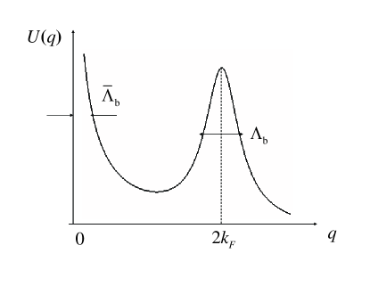
Figure 1: A model interaction potential with two cutoffs: ${\bar{\Lambda}}_{\mathrm{b}}$ near $q=0$ and $\Lambda_{\mathrm{b}}$ near $q=2k_{F}$.

We consider an effective low-energy model of 1D fermions with a linearized fermionic dispersion $\epsilon_{k}$ near $\pm k_{F}$, $\epsilon_{k}=\pm v_{F}(k\mp k_{F})$, and with a short-range four-fermion interaction $U(q)$. We set a fermionic momentum cutoff at a scale $\Lambda_{\mathrm{f}}$ (generically, comparable to the lattice constant) , and assume that fermions with energies larger than $v_{F}\Lambda_{\mathrm{b}}$ account for the renormalization of the bare interaction into an effective one, which acts between low-energy fermions, and depends not only on transferred momentum, but also on two incoming fermionic momenta. We then use the $g$-ology notations giamarchi_book , and introduce three dimensionless vertex functions, $g_{1}$, $g_{2}$ and $g_{4}$, which describe scattering processes along the Fermi surface with zero incoming and $2k_{F}$ transferred momenta, zero incoming and zero transferred momenta, and $2k_{F}$ incoming and zero transferred momenta, respectively. At first order in the interaction, $g_{1}=U(2k_{F})/(2\pi v_{F})$, $g_{2}=g_{4}=U(0)/(2\pi v_{F})$. The effective low-energy model only makes sense if the couplings $g_{i}$ vanish long before the scale of $\Lambda_{\mathrm{f}}$, otherwise the low-energy and high-energy sectors could not be separated. A way to enforce this constraint, which we will adopt, is to assume that the interactions $g_{i}$ are non-zero only for transferred momenta (either around zero or $2k_{F}$), which are smaller than $\Lambda_{\mathrm{f}}$. Accordingly, we introduce two “bosonic” cutoffs: $\Lambda_{\mathrm{b}}$, set by the interaction with the momentum transfer near $2k_{F}$ ($g_{1}$ vertex), and ${\bar{\Lambda}}_{\mathrm{b}}$, set by the interaction with a small momentum transfer ($g_{2}$ and $g_{4}$ vertices), and request that both are smaller than $\Lambda_{\mathrm{f}}$. More precisely, we assume that

$$\Lambda_{\mathrm{f}}-\Lambda_{\mathrm{b}},\Lambda_{\mathrm{f}}-{\bar{\Lambda}}_{\mathrm{b}}\gg T.$$ (2)

The model interaction is shown in Fig. 1. We will see that there is an interesting dependence of the specific heat on the ratio $\Lambda_{\mathrm{b}}/\Lambda_{\mathrm{f}}$, but no dependence on the ratio ${\bar{\Lambda}}_{\mathrm{b}}/\Lambda_{\mathrm{f}}$.

The two-cutoff model with $\Lambda_{\mathrm{b}}<\Lambda_{\mathrm{f}}$ has been used in the canonical 1D bosonization approach, and in the subsequent analysis of the sine-Gordon model. It was also considered in Refs.twocutoffs, ; grest, in the analysis of the electron-phonon interaction in 1D. We note in passing that, to our knowledge, it has not been explicitly verified that the specific heat for the effective low-energy model is the same as for the original model of fermions with parabolic-type dispersion and a generic interaction $U(q)$, i.e., that all contributions to $C(T)$ from fermionic energies exceeding $\Lambda_{\mathrm{f}}$ can be absorbed into the three couplings $g_{i}$. We also note that, in the bosonization procedure invented by AE, which is not based on the $g-$ology model, the cutoff imposed by the interaction is less restrictive that the fermionic cutoff (i.e., $\Lambda_{\mathrm{b}}\gg\Lambda_{\mathrm{f}}$), because in their theory the propagators of long-wavelength bosonic modes are obtained by integrating independently over fermionic momenta linked by the interaction. AE, however, only focused on the truly low-energy terms with the running coupling, which should not depend on the ratio $\Lambda_{\mathrm{b}}/\Lambda_{\mathrm{f}}$.

Vertices $g_{1}$ and $g_{2}$ in the $g$ -ology model are related to the spin and charge components of the backscattering amplitude

$$f_{\alpha\beta,\gamma\delta}(\pi)=f_{c}(\pi)\delta_{\alpha\beta}\delta_{\gamma\delta}+f_{s}(\pi){\vec{\sigma}}_{\alpha\beta}\cdot{\vec{\sigma}}_{\gamma\delta},$$ (3)

as $f_{c}(\pi)=2g_{2}-g_{1}$, $f_{s}(\pi)=-g_{1}$. Vertex $g_{4}$ is related to the forward scattering amplitude $f(0)$ as $g_{4}=f_{c}(0)-f_{s}(0)$. For generality, we extend the model from the $SU(2)$ symmetric to anisotropic case, i.e., assume that all three vertex functions $g_{i}$ ($i=1,2,4$) have different values $g_{i\parallel}$ and $g_{i\perp}$, depending on whether the spins of the fermions in the initial state are parallel or opposite. For anisotropic case, the spin component of the backscattering amplitude splits into the longitudinal and transverse parts, and we have

$$f_{c}(\pi) = g_{2\parallel}-g_{1\parallel}+g_{2\perp},$$

$$f_{s\parallel}(\pi) = g_{2\parallel}-g_{1\parallel}-g_{2\perp},$$

$$f_{s\perp}(\pi) = -g_{1\perp}.$$ (4)

The forward scattering vertex $g_{4}$ is invariant under RG renormalization, but the backscattering vertices $g_{1}$ and $g_{2}$ flow solyom ; emery . Keeping only the processes with momentum transfers in narrow windows near either zero or $2k_{F}$ (the windows are much smaller than the cutoffs $\Lambda_{\mathrm{b}}$ and ${|bar\Lambda}_{b}$), we have

$$\frac{dg_{1\parallel}}{dL}=\beta_{1\parallel};~{}~{}\frac{dg_{1\perp}}{dL}=\beta_{1\perp}$$

$$\frac{dg_{2\parallel}}{dL}=\beta_{2\parallel};~{}~{}\frac{dg_{2\perp}}{dL}=\beta_{2\perp}$$ (5)

where $L=\log E_{F}/E$, $E$ is the running energy, and $\beta$ functions depend on the couplings $g_{1\parallel,\perp}$ and $g_{2\parallel,\perp}$. In the one-loop approximation,

$$\beta_{1\parallel}=-(g^{2}_{1\parallel}+g^{2}_{1\perp}),~{}~{}\beta_{1\perp}=-2g_{1\perp}\left(g_{1\parallel}-g_{2\parallel}+g_{2\perp}\right),$$

$$\beta_{2\parallel}=-g^{2}_{1\parallel},~{}~{}\beta_{2\perp}=-g^{2}_{1\perp}.$$ (6)

Re-expressing the couplings in terms of spin and charge components of the backscattering amplitude, we find that the spin amplitudes $f_{s_{\parallel}}$ and $f_{s\perp}$ flow to zero under the RG transformation. The charge component of the backscattering amplitude $f_{c}(\pi)=(g_{2\parallel}+g_{2\perp})-g_{1\parallel}$, however, does not change under the RG flow.

For the SU(2) symmetric case, $\beta_{1}=-2g^{2}_{1}/(1-g_{1}),~{}\beta_{2}=\beta_{1}/2$, and $g_{1}(L)$ renormalizes to zero as $1/L$, while $g_{2}(L)$ tends to a constant value of a half of the charge amplitude, which is invariant under RG.

As we said earlier, the key interest of our analysis is to understand at which order within the $g-$ology model the running couplings appear in the specific heat, and what are the contributions to the specific heat which contain bare couplings.

I.2 Results

We first catalog our main results, and then present calculations in the bulk of the paper. We computed $C(T)$ in a direct perturbation theory, expanding in powers of the couplings $g_{i}$ to order $g^{3}$. To first two orders in $g_{i}$, we found that the specific heat is expressed via bare couplings $g_{2}$ and $g_{4}$, and the effective backscattering coupling $g_{1}$. At third order, we found an extra contribution to $C(T)$, which comes from low-energies and contains a cube of the running backscattering amplitude on the scale of $T$. Explicitly, for the anisotropic case, we found for $T\ll\Lambda_{\mathrm{b}}$ and neglecting $O(g^{3})$ contributions with non-running couplings

$$C(T)=\frac{2\pi T}{3v_{F}}~{}\left[1+\left({\tilde{g}}_{1\parallel}-g_{4\parallel}\right)+\left({\tilde{g}}_{1\parallel}-g_{4\parallel}\right)^{2}+g^{2}_{4\perp}+\frac{1}{2}\left((g^{2}_{2\parallel}+g^{2}_{2\perp})-2g_{2\parallel}{\tilde{g}}_{1\parallel}+({\tilde{g}}^{2}_{1\parallel}+{\tilde{g}}^{2}_{1\perp})\right)+3{\tilde{g}}^{2}_{1\perp}(T){\tilde{g}}_{1\parallel}(T)+...\right],$$ (7)

Here $g_{4}$ and $g_{2}$ are the bare couplings, and ${\tilde{g}}_{1\parallel}$ and ${\tilde{g}}_{1\perp}$ are the effective couplings on the scale $\Lambda_{\mathrm{b}}$. The couplings ${\tilde{g}}_{1\parallel}(T)$ and ${\tilde{g}}_{1\perp}(T)$ are running couplings on the scale of $T$ – these are the solutions of the full RG equations, Eq. (5), with effective ${\tilde{g}}_{1\parallel}$ and ${\tilde{g}}_{1\perp}$ serving as inputs.

Figure 2: One-loop diagrams for the interaction vertices. In the RG regime (external momenta are much smaller than $\Lambda_{b}$), the renormalizations of $g_{1\perp}$ and $g_{1\parallel}$ are given by diagrams a), b), and d), while the renormalizations of $g_{2\perp}$ and $g_{2\parallel}$ are given by diagrams c) and d). All diagrams give rise to $\log T$ terms. For external momenta of order $\Lambda_{b}$, only diagram a) gives rise to the logarithmic term $\log\left(\Lambda_{{\rm f}}/\Lambda_{{\rm b}}\right)$, as the two fermions in the particle-hole bubble can have momenta in the whole range between $\Lambda_{{\rm b}}$ and $\Lambda_{{\rm f}}$. For all other diagrams, the interaction constraints the internal momenta to be of the same order as the external momentum, and there is no momentum space for the logarithm.

The effective couplings ${\tilde{g}}_{1\parallel}$ and ${\tilde{g}}_{1\perp}$ differ from bare $g_{1\parallel,\perp}$ due to RPA-type renormalizations by $2k_{F}$ particle-hole bubbles made of fermions with momenta between $\Lambda_{\mathrm{b}}$ and $\Lambda_{\mathrm{f}}$. This renormalization comes from diagram a) in Fig. 2). There are no such renormalizations for $g_{2}$ couplings, which retain their bare values. We obtain

$${\tilde{g}}_{1\parallel}\!=\!g_{1\parallel}\!-\!\left(g^{2}_{1\parallel}+g^{2}_{1\perp}\right)L_{\rm{b}}\!+\!\left(g^{3}_{1\parallel}\!+\!3g_{1\parallel}g^{2}_{1\perp}\right)L^{2}_{b}$$ (8a)

$${\tilde{g}}^{2}_{1\parallel}+{\tilde{g}}^{2}_{1\perp}=g^{2}_{1\parallel}+g^{2}_{1\perp}-2\left(g^{3}_{1\parallel}+3g_{1\parallel}g^{2}_{1\perp}\right)L_{\rm{b}}$$ (8b)

where $L_{\mathrm{b}}=\log{\left(\Lambda_{\mathrm{f}}/\Lambda_{\mathrm{b}}\right)}$.

We emphasize that an RPA-type renormalization is not equivalent to RG, so that effective ${\tilde{g}}_{1\parallel}$ and ${\tilde{g}}_{1\perp}$ differ from the solutions of (5), (6) already at one-loop order. The difference is due to the fact that in the one-loop RG equations, the RPA and ladder-type renormalizations of $g_{1}$, and the ladder renormalizations of $g_{2}$ are all coupled, while only the RPA diagrams lead to $L_{\rm{b}}$ terms in the renormalization from $g_{1}$ to ${\tilde{g}}_{1}$ .

Coupling between the RPA and ladder renormalizations in the RG regime is absent for the isotropic, $SU(2)$ symmetric case. Then ${\tilde{g}}_{1}=g_{1}/(1+2g_{1}L_{\mathrm{b}})$ becomes equivalent to one-loop RG. Furthermore, in the symmetric case, the running $g_{1}(L)$ at the lowest energies behaves in the one-loop approximation as ${\tilde{g}}_{1}/(1+2{\tilde{g}}_{1}L)$. For the specific heat we then obtain

$$C(T)=\frac{2\pi T}{3v_{F}}~{}\left[1+\left({\tilde{g}}_{1}-g_{4}\right)+\left({\tilde{g}}_{1}-g_{4}\right)^{2}+g^{2}_{4}+\left(g_{2}-\frac{1}{2}{\tilde{g}}_{1}\right)^{2}+\frac{3}{4}\tilde{g}_{1}^{2}+\frac{3{\tilde{g}}_{1}^{3}}{(1+2{\tilde{g}}_{1}L)^{3}}\right]$$ (9)

The results of our direct perturbative analysis are in agreement with the results for the Kondo problem kondo and XXZ spin chain lukyanov – for both models, the specific heat was shown to behave as $T/\log^{3}T$ at the lowest temperatures. These two models are argued to be in the same universality class as the model of interacting electrons with the interaction in the spin sector. The same behavior was found by Cardy cardy and Ludwig and Cardy ludwig_cardy in their study of a conformally invariant theory perturbed by the marginal perturbation from the fixed point (the sine-Gordon model belongs to this class of theories), and by AE in their “multidimensional bosonization” analysis. In all these theories, the focus was on the universal terms which are confined to low energies i.e., are not anomalies. If only such terms are included, the full spin contribution to the specific heat scales as $T/\log^{3}T$ in the $SU(2)$ isotropic case, i.e., the spin part of the specific heat coefficient vanishes at $T=0$. Our direct perturbation theory reproduces the same universal behavior in the spin sector, but also generates extra contributions to the specific heat which contain effective interaction on the scale of $\Lambda_{\mathrm{b}}$.

To make the comparison with the bosonization and sine-Gordon model explicit, we re-write our result via spin and charge velocities $v_{F}u_{\rho}$ and $v_{F}u_{\sigma}$ obtained by diagonalizing the gradient part of the Hamiltonian:

$$u_{\rho}^{2}\!=\!(1+g_{4\parallel}+g_{4\perp}-g_{1\parallel})^{2}\!-\!(g_{2\parallel}+g_{2\perp}-g_{1\parallel})^{2},$$

$$u_{\sigma}^{2}\!=\!(1+g_{4\parallel}-g_{4\perp}-g_{1\parallel})^{2}\!-\!(g_{2\parallel}-g_{2\perp}-g_{1\parallel})^{2}$$ (10)

Using (10), one can re-write (7) as

$$C(T)=\frac{\pi T}{3v_{F}}\left(\frac{1}{{\tilde{u}}_{\rho}}+\frac{1}{{\tilde{u}}_{\sigma}}\right)+\frac{\pi T}{3v_{F}}{\tilde{g}}_{1\perp}^{2}+\frac{2\pi T}{v_{F}}~{}g^{2}_{1\perp}(T)g_{1\parallel}(T).$$ (11)

The last term in (11) is the universal contribution from low energies. The first term is the sum of the specific heats of two gases of free particles with the effective velocities ${\tilde{u}}_{\rho}$ and ${\tilde{u}}_{\sigma},$ which are the same as in (10) except for $g_{1||}$ and $g_{1\perp}$ are now the effective, renormalized vertices. The term in the middle is an additional contribution from the spin channel. Very likely, this contribution can be absorbed into the renormalization of spin velocity ${\tilde{u}}_{\sigma}\rightarrow{\tilde{u}}_{\sigma}-{\tilde{g}}_{1\perp}^{2}$, i.e., the specific heat can be re-expressed as the sum of the contribution with running couplings, and the specific heat of two ideal gases of fermions with bare charge velocity (albeit with ${\tilde{g}}_{1}$), and the renormalized spin velocity.

In the rest of the paper, we present the details of our calculations. In Sec. II.2, we outline the computational procedure, calculate the first-order diagram for the thermodynamic potential, and demonstrate explicitly the sensitivity of the result for $C(T)$ to the ratio of the cutoffs. In Sec.II.3 and II.4, we compute second and third order diagrams for the thermodynamic potential, and discuss the fourth-order result. In Sec.III, we analyze the specific heat in the framework of the sine-Gordon model. Sec. IV presents the conclusions. Some technical details of the calculations are presented in the Appendices.

II Perturbation theory and the role of cutoffs

II.1 Preliminaries

In this and the next two Sections we set $v_{F}=1$. We restore $v_{F}$ in the final formulas for the specific heat.

The specific heat of an interacting system of fermions can be extracted from the thermodynamic potential $\Xi$ via $C(T)=-T\partial^{2}\Xi/\partial T^{2}$. The thermodynamic potential is given by the Luttinger-Ward formula:

$$\Xi=\Xi^{(0)}-2T\sum_{\omega}\int\frac{dk}{2\pi}\left[\log\left(G_{0}G^{-1}\right)-\Sigma G+\sum_{\nu}\frac{1}{2\nu}\Sigma_{\nu}G\right]$$ (12)

where

$$\Xi^{(0)}=-2T\sum_{\omega}\int\frac{dk}{2\pi}\left[\frac{1}{2}\log\left(\epsilon_{\mathbf{k}}^{2}+\omega_{m}^{2}\right)\right],$$ (13)

is the thermodynamic potential of the free Fermi gas per unit length $G_{0}=\left(i\omega_{m}-\epsilon_{k}\right)^{-1}$, $\epsilon_{k}$ is the dispersion, $G=\left(i\omega_{m}-\epsilon_{k}+\Sigma\right)^{-1}$, $\Sigma$ is the exact (to all orders in the interaction) self-energy, and $\Sigma_{\nu}$ is the skeleton self-energy of order $\nu$. The skeleton and full self-energy are related via $\Sigma=\sum_{\nu}\Sigma_{\nu}$ and are evaluated at finite $T$. Expanding both $G$ and $\Sigma_{\nu}$ in Eq. (11) in powers of the interaction, one generates a perturbative expansion for $\Xi$ in the series of closed diagrams with no external legs.

The free-fermion expression for $C(T)$ is obtained from Eq. (13). At low $T$, the momentum integration is confined to $k\approx\pm k_{F}$ and yields

$$\Xi^{(0)}=-T\sum_{\omega_{m}}|\omega_{m}|=-\frac{\pi T^{2}}{3}+{\text{c}onst},$$ (14)

such that $C^{(0)}(T)=2\pi T/3$.

II.2 First order diagrams

Figure 3: First order diagrams for the thermodynamic potential. Here and in the rest of the figures, the dashed line represents the interaction. Diagram 1b) does not contribute to the temperature dependence of the thermodynamic potential.

At first order, the $T$ dependence of $\Xi$ comes from the bubble diagram crossed by the interaction line [diagram 1a) in Fig.3). This diagram contains two contributions: one with a small momentum transfer and another with a momentum transfer near $2k_{F}$. As spin is conserved along the bubble, the corresponding coupling constants are $g_{4\parallel}$ and $g_{1\parallel},$ respectively.

The safe way to evaluate the diagram is to sum over frequencies first, as the frequency summation is constrained neither by the interaction nor by the fermionic bandwidth, and then integrate over the fermionic momentum $k$ and bosonic, transferred momentum $q$. We will measure $q$ as a deviation from zero for $g_{4\parallel}$ term, and from $2k_{F}$ for $g_{1\parallel}$ term, and, as we said, will cut interactions at $|q|={\bar{\Lambda}}_{\mathrm{b}}$ for forward scattering process and at $\Lambda_{\mathrm{b}}$ for backscattering process. We linearize the fermionic dispersion near the Fermi surface and set the cutoff of the integration over $k$ at $|k\pm q/2|\leq\Lambda_{\mathrm{f}}$, $\Lambda_{\mathrm{f}}>{\bar{\Lambda}}_{\mathrm{b}},\Lambda_{\mathrm{b}}$.

For small momentum transfer, we then obtain

$$\Xi^{(1)}_{q=0}=\frac{2g_{4\parallel}}{\pi}\int_{0}^{{\bar{\Lambda}}_{\mathrm{b}}}\!\!\!\!dq\int_{0}^{\Lambda_{\mathrm{f}}-q/2}\!\!\!\!dk\frac{\cosh{\frac{q}{2T}}}{\cosh{\frac{q}{2T}}+\cosh{\frac{k}{T}}},$$ (15)

and for the momentum transfer near $2k_{F}$, we obtain

$$\Xi^{(1)}_{2k_{F}}=\frac{2g_{1\parallel}}{\pi}\int_{0}^{\Lambda_{\mathrm{b}}}\!\!\!\!dq\int_{0}^{\Lambda_{\mathrm{f}}-q/2}\!\!\!\!dk\frac{\cosh{\frac{k}{T}}}{\cosh{\frac{q}{2T}}+\cosh{\frac{k}{T}}}.$$ (16)

Subtracting $T$-independent terms in (15) and (16) and introducing rescaled variables $x=k/T$, $y=q/(2T)$, we re-write (15) and (16) as

$$\Xi^{(1)}_{q=0} = \frac{2g_{4\parallel}T^{2}}{\pi}\int_{0}^{{\bar{\Lambda}}_{\mathrm{b}}/2T}\!\!\!\!dy\int_{0}^{\frac{\Lambda_{\mathrm{f}}}{T}-y}\!\!\!\!dx\frac{\cosh{y}-\cosh{x}}{\cosh{y}+\cosh{x}},$$ (17)

and

$$\Xi^{(1)}_{2k_{F}}=\frac{2g_{1\parallel}T^{2}}{\pi}\int_{0}^{\Lambda_{\mathrm{b}}/2T}\!\!\!\!dy\int_{0}^{\frac{\Lambda_{\mathrm{f}}}{T}-y}\!\!\!\!dx\frac{\cosh{x}-\cosh{y}}{\cosh{x}+\cosh{y}}.$$ (18)

We immediately see that the first-order contribution to the thermodynamic potential vanishes if we formally extend the integrals over $x$ and $y$ to infinity. Integrals (17) and (18) are similar to the integrals which give rise to anomalies in the field theory jackiw . The integrands are odd under the interchange of $x$ and $y$; therefore universal, cutoff independent contributions apparently vanish, but the 2D integrals are ultraviolet divergent, if we set $T$ to zero. A finite $T$ then sets an ultraviolet regularization of the divergent 2D integral and gives rise to finite terms in $\Xi$ which do not explicitly depend on the cutoff. By analogy with the field theory, hereafter we refer to these terms as “anomalies”.

For definiteness, we focus on the $2k_{F}$ contribution. Since $\Lambda_{\mathrm{f}}>\Lambda_{\mathrm{b}}$ (in the sense of Eq.(2), the integration over $y$ extends to a much narrower range than that over $x$. In this situation, the most natural way to evaluate the thermal part of $\Xi^{(1)}_{2k_{F}}$ is to re-express (18) as

$$\Xi^{(1)}_{2k_{F}}=-\frac{4}{\pi}g_{1\parallel}T^{2}\int_{0}^{\Lambda_{\mathrm{b}}/2T}dy\cosh{y}$$

$$\times\int_{0}^{\frac{\Lambda_{\mathrm{f}}}{T}-y}\frac{dx}{\cosh{x}+\cosh{y}}.$$ (19)

The integral over $x$ now converges, and, because $\Lambda_{\mathrm{f}}>\Lambda_{\mathrm{b}}$, we can safely set the upper limit of the $x$ integral to infinity. The $x$ integration then can be performed exactly and yields

$$\Xi^{(1)}_{2k_{F}}=-\frac{4}{\pi}~{}g_{1\parallel}T^{2}\int_{0}^{\Lambda_{\mathrm{b}}/2T}dyy\coth{y},$$ (20)

$$= -\frac{g_{1\parallel}}{2\pi}\Lambda_{b}^{2}-\frac{4g_{1\parallel}}{\pi}T^{2}\int_{0}^{\Lambda_{\mathrm{b}}/2T}dyy(\coth{y}-1).$$

The thermal part of $\Xi^{(1)}_{2k_{F}}$ comes from the second term

$$\Xi^{(1)}_{2k_{F}}=\mathrm{const}-\frac{\pi}{3}g_{1\parallel}T^{2}.$$ (21)

Observe that the $T^{2}$ piece is independent of the cutoff. Furthermore, in this computational procedure, the frequency sums and the momentum integrals are fully ultraviolet convergent, and Eq. (21) comes from small momenta $k,q\sim T\ll\Lambda_{\mathrm{f}},$ $\Lambda_{\mathrm{b}}$.

Alternatively, however, we can evaluate the integrals in (18) by integrating over the (dimensionless) bosonic momentum $y$ first. To do this, we neglect $y$ in the upper limit of the integral over $x$ (we will check a’posteriori that this is justified), and re-express (18) as

$$\Xi^{(1)}_{2k_{F}}=\frac{4g_{1\parallel}}{\pi}T^{2}\int_{0}^{\Lambda_{\mathrm{f}}/T}dx\cosh{x}$$

$$\times\int_{0}^{\Lambda_{\mathrm{b}}/2T}\frac{dy}{\cosh{x}+\cosh{y}}.$$ (22)

It is tempting to set the upper limit of the $y$ integral to infinity, as this integral converges. However, one has to be cautious as there is a range of $x$ where $\cosh{x}>\cosh{y}$ for any $y$. To see how this affects the result, we represent the $y$ integral as

$$\int^{\Lambda_{\mathrm{b}}/2T}_{0}\frac{dy}{\cosh{x}+\cosh{y}}=\int^{\infty}_{0}\frac{dy}{\cosh{x}+\cosh{y}}-\int^{\infty}_{\Lambda_{\mathrm{b}}/2T}\frac{dy}{\cosh{x}+\cosh{y}}=\frac{x}{\sinh{x}}-\frac{1}{\cosh{x}}\int^{\infty}_{\left(\Lambda_{\mathrm{b}}/2T\right)}\frac{dy}{1+e^{y-x}}.$$ (23)

We replaced $\cosh{x}$ and $\cosh{y}$ in the last term by the exponentials, as $y$ are large, and we anticipate typical $x$ to be large as well. The remaining integration is straightforward, and we obtain

$$\Xi^{(1)}_{2k_{F}}={\rm const}+\frac{\pi}{3}g_{1\parallel}T^{2}-\frac{4g_{1\parallel}}{\pi}T^{2}\int^{\Lambda_{\mathrm{f}}/T}_{0}dx\log\left(1+e^{x-\Lambda_{\mathrm{b}}/2T}\right).$$ (24)

The first term is the contribution from low energies – the same as in (21), but with the opposite sign. The second term by construction is the contribution from energies much larger than $T$. Evaluating the second integral, we find that it also contributes a $T^{2}$ term to $\Xi^{(1)}_{2k_{F}}$:

$$\frac{4g_{1\parallel}}{\pi}T^{2}\int_{0}^{\Lambda_{\mathrm{f}}/T}dx\log\left(1+e^{x-\Lambda_{\mathrm{b}}/2T}\right)$$ (25)

$$= \mathrm{const}+\frac{2\pi}{3}g_{1\parallel}T^{2},$$

The $T^{2}$ term in (25) comes from $x\sim\Lambda_{\mathrm{b}}/2T$. It is essential that these $x$ are smaller than the upper limit of $x-$integration, otherwise such a contribution would not exist. Substituting this back into (24), we find that the high-energy term is opposite in sign and twice larger than the low-energy one, so that the sum of the two contributions is given precisely by Eq.(21). Going back through the derivation of (25), we see that typical $y$ and $x$ are near $\Lambda_{\mathrm{b}}/2T$, well below the upper limit of the $x$ integration. In this situation, the neglect of $y$ in the upper limit of the integral over $x$ is legitimate, to accuracy $\exp{-\Lambda_{\mathrm{b}}/T}$.

We see therefore that $\Xi^{(1)}_{2k_{F}}$ can be equally well obtained either as a low-energy contribution or as a high-energy one. This is a hallmark of an anomaly. The same is true also for the forward scattering term $\Xi^{(1)}_{q=0}$: the $T^{2}$ term again can be equally obtained as a low-energy contribution or as a contributions from energies of order ${\bar{\Lambda}}_{\mathrm{b}}$.

Combining the results for backscattering and forward scattering, we obtain for the specific heat

$$C^{(1)}(T)=\frac{2\pi T}{3v_{F}}\left(~{}g_{1\parallel}-g_{4\parallel}\right).$$ (26)

As we said in the Introduction, the $g_{1\parallel}$ term in (26) is not present in the standard bosonization approach giamarchi_book . The physical argument is that the $g_{1\parallel}$ should only appear in $C(T)$ in the combination $g_{1\parallel}-g_{2\parallel}$ as the two vertices transform into each other by interchanging external momenta without interchanging spins, and therefore are physically indistinguishable schulz_95 ; metzner . The first order diagram with $g_{2\parallel}$ is a Hartree diagram with two bubbles connected by the interaction at exactly zero transferred momentum [diagram 1b) in Fig.3]. As each of these two bubbles represents a total electron density, this diagram obviously does not depend on $T$. By the argument above, the diagram with $g_{1\parallel}$ also should not depend on $T$. This consideration is, however, only valid if the cutoffs are infinite. For finite cutoffs, there appears an extra “anomaly-type” contribution, in which $g_{1\parallel}$ appears in the combination with $g_{2\parallel}$, as we just demonstrated  kostya_private . A similar reasoning within real-space consideration has been presented in capponi . Another argument for presence of the $g_{1\parallel}$ term is based on the observation that fermions with the same spin do not interact via a contact interaction; hence the interaction should drop out of the results in this limit. This implies that the observables, such as $C(T)$ must depend separately on the combinations $g_{4||}-g_{1||}$ and $g_{2||}-g_{1||}$  starykh_maslov ; matveev . Eq. (26) is consistent with this argument as the limit of a contact interaction, i.e, for $g_{1\parallel}=g_{4\parallel}$, $C^{(1)}(T)$ vanishes.

The interplay between low-energy and high-energy contributions to $\Xi$ can be also understood if one interchanges one momentum integration and one frequency summation and expresses $\Xi^{(1)}$ via the polarization bubble as

$$\Xi^{(1)}_{q=0}=-g_{4\parallel}T\sum_{\Omega}\int dq\Pi_{q=0}(q,\Omega),$$

$$\Xi^{(1)}_{2k_{F}}=-g_{1\parallel}T\sum_{\Omega}\int_{-\Lambda_{\mathrm{b}}}^{\Lambda_{\mathrm{b}}}dq\Pi_{2k_{F}}(q,\Omega).$$ (27)

The sub-indices indicate that the momentum integration is confined to $q$ near zero or near $2k_{F}$.

For briefness, we consider only the backscattering term. The polarization bubble $\Pi_{2k_{F}}(q,\Omega)$ is given by

$$\Pi_{2k_{F}}(q,\Omega) \equiv 2T\sum_{\omega}\int\frac{dk}{2\pi}G_{R}(\omega+\Omega,k+q)G_{L}(\omega,k)+G_{L}(\omega+\Omega,k+q)G_{R}(\omega,k)$$ (29)

$$=\frac{1}{2\pi}\left(\log{\frac{\Omega^{2}+q^{2}}{4\Lambda^{2}_{f}}}-8\int_{0}^{\infty}dkkn_{F}(k)\left(\frac{1}{(q-i\Omega)^{2}-4k^{2}}+\frac{1}{(q+i\Omega)^{2}-4k^{2}}\right)\right),$$

where $G_{L,R}(k\omega)$ is the Green’s function of right/left moving fermions and $n_{F}(x)$ is the Fermi function. The first term in Eq.(29) is the zero-temperature Kohn anomaly, the rest is the thermal contribution. The integration over $k$ gives the result for $\Pi(q,\Omega)$ in terms of di-Gamma functions schulz , but for our purposes it is more convenient to use (29).

Substituting (29) into (27), we find

$$\Xi^{(1)}_{2k_{F}}=-g_{1\parallel}~{}(Q+P),$$ (30)

where $Q$ and $P$ are the contributions from the Kohn anomaly and from the thermal piece in (29), respectively. The temperature -dependent part of the $Q$ term is

$$Q=\frac{1}{2\pi}~{}T\sum_{\Omega}\int_{-\Lambda_{\mathrm{b}}}^{\Lambda_{\mathrm{b}}}dq\log{\frac{\Omega^{2}+q^{2}}{4\Lambda^{2}_{f}}},$$ (31)

comes from low energies regardless of whether the sum or the integral is done first. In both cases, we get, up to a constant,

$$Q=Q_{L}=-\pi T^{2}/3,$$ (32)

where subindex L specifies that this is a contribution from low energies: $\Omega,q\sim T$. The second, thermal, term is determined either by low or by high energies, depending on the order. If the momentum integration is done first, the non-zero result is obtained only because $\Lambda_{\mathrm{b}}$ is finite; otherwise, the integration contour can be closed in that half-plane where the integrand has no poles. Re-arranging the integrals, we rewrite this contribution as

$$P=-\frac{4}{\pi}T\sum_{\Omega}\int^{\Lambda_{\mathrm{b}}}_{-\Lambda_{\mathrm{b}}}dq\int_{0}^{\infty}dkkn_{F}(k)\left(\frac{1}{(q-i\Omega)^{2}-4k^{2}}+\frac{1}{(q+i\Omega)^{2}-4k^{2}}\right),$$

$$=\frac{8}{\pi}T\sum_{\Omega}\int^{\infty}_{\Lambda_{\mathrm{b}}}dq\int_{0}^{\infty}dkkn_{F}(k)\left(\frac{1}{(q-i\Omega)^{2}-4k^{2}}+\frac{1}{(q+i\Omega)^{2}-4k^{2}}\right).$$ (33)

As the Fermi function in (29) confines the fermionic momentum to $k\sim T$, and $q>\Lambda_{\mathrm{b}}$ is large, we can neglect $4k^{2}$ compared to $(q\pm i\Omega)^{2}$ in the denominator. This simplifies $P$ to

$$P=\frac{2\pi T^{2}}{3}T\sum_{\Omega}\int_{\Lambda_{\mathrm{b}}}^{\infty}dq\left(\frac{1}{(q-i\Omega)^{2}}+\frac{1}{(q+i\Omega)^{2}}\right)$$ (34)

Performing the momentum integration, we obtain

$$P=\frac{4\pi T^{2}}{3}T\sum_{\Omega}\frac{\Lambda_{\mathrm{b}}}{\Lambda_{\mathrm{b}}^{2}+\Omega^{2}}.$$ (35)

Evaluating the integral, we find that $P$ does not depend on the cutoff, and equals to

$$P=P_{H}=\frac{2\pi T^{2}}{3},$$ (36)

where subindex $H$ specifies that this is a contribution from high energies $\Omega,q\sim\Lambda_{\mathrm{b}}$.

Alternatively, $P$ can be evaluated by doing frequency summation first. One can easily check that, to order $T^{2}$, the frequency sum can be replaced by the integral. The frequency integral is non-zero only for $q<2k$, otherwise the poles in $\Omega$ are located in the same half-plane, and the frequency integral vanishes. Evaluating the frequency integral and then the integral over $q$, we reduce $P$ to

$$P=P_{L}=\frac{8}{\pi}\int_{0}^{\infty}dkkn_{F}(k)=\frac{2\pi T^{2}}{3},$$ (37)

where subindex $L$ specifies that this a contribution from low energies $\Omega\sim T$. We see that $P_{H}=P_{L}$, i.e., the same result for $P$ can be obtained either as a high-energy contribution, or as low-energy one. In both cases $P$ is formally independent of the cutoff, and the total backscattering part of $\Xi^{\left(1\right)}$ is given by

$$\Xi^{(1)}_{2k_{F}}=\mathrm{const}-g_{1\parallel}(Q+P)=\mathrm{const}-\frac{g_{1\parallel}\pi}{3}T^{2},$$ (38)

which coincides with (21).

Which of the two ways (low-energy or high-energy) is physically correct? As we discussed in the Introduction, if $\Xi^{(1)}_{2k_{F}}$ comes from low energies (of order $T$), one should expect $T\log T$ terms in $C(T)$ already at the next (second) order; on the contrary, if it comes from high energies, no such terms are expected. AE suggested implicitly that the correct procedure is to take the average of two possible orderings, i.e., to represent frequency summation and momentum integration in (27) as

$$\frac{1}{2}\left(T\sum_{\Omega}~{}\int dq+\int dq~{}T\sum_{\Omega}\right).$$ (39)

In this procedure, $P$ in Eq. (33) is a sum

$$P=\frac{1}{2}P_{L}+\frac{1}{2}P_{H},$$ (40)

with $P_{H}=P_{L}=\pi T^{2}/3$. Total $\Xi^{(1)}_{2k_{F}}$ is the sum of $P$ and $Q$ [see Eq.(38)], where $Q=Q_{L}=-\pi T^{2}/3$ comes from low energies. Adding $P$ and $Q$, we find that the low-energy contributions cancel out, and the net result for $\Xi^{(1)}_{2k_{F}}$ is the high-energy contribution.

Eq. (39), however, contains some ambiguity, as one could equally well can re-write $P$ as $\alpha P_{L}+(1-\alpha)P_{H}$ with an arbitrary coefficient $\alpha$. Then, the balance between the low and high energy contributions to $\Xi^{\left(1\right)}$ would depend on $\alpha$. Whether $\Xi^{\left(1\right)}$ contains running or bare coupling $g_{1||}$ can only be established by an explicit computation to the next (second) order. This is what we will do in next Section.

II.3 Second order diagrams

Figure 4: Second order diagrams for the thermodynamic potential.

The second-order diagrams for the thermodynamic potential are shown in Fig. 4. There are two different types of diagrams, obtained by inserting either self-energy corrections or vertex corrections into the first-order diagram. The diagram with self-energy insertions [diagram 2a)] is readily computed either explicitly, or by evaluating first-order self-energy and substituting the result into the first-order diagram. We will not discuss computational steps (they are not qualitatively different from those to first order) and present only the final result: the diagram 2a) yields a regular $T^{2}$ contribution to $\Xi$ of the form

$$\Xi_{2a}^{(2)}=-\frac{1}{3\pi}T^{2}\left(g_{1\parallel}-g_{4\parallel}\right)^{2}.$$ (41)

Next, there are vertex correction diagrams 2b) and 2c), which involve the forward scattering vertex $g_{4}$ (small transferred momentum and $2k_{F}$ total incoming momentum) and $g_{2}$ vertex (small transferred and small total incoming momentum). The contributions of order $g_{4\parallel}^{2}$, $g_{4\perp}^{2}$, $g_{2\parallel}^{2}$, $g_{2\perp}^{2}$, and also of order $g_{2\parallel}g_{1\parallel}$, are all expressed via the bilinear combinations of the bubbles for right and left movers

$$\Pi_{L,R}(q,\Omega) \equiv T\sum_{\omega}\int\frac{dk}{2\pi}G_{R,L}(k+q,\omega+\Omega)G_{R,L}(k,\omega)$$ (42)

$$= \pm\frac{1}{2\pi}\frac{q}{\imath\Omega\mp q},$$

whose sum is the total polarization bubble $\Pi_{q=0}(q,\Omega)=\Pi_{R}(q,\Omega)+\Pi_{L}(q,\Omega).$ The evaluation of $T\sum_{\Omega}\int dq\Pi_{i}(q,\Omega)\Pi_{j}(q,\Omega)$ ($i,j=L,R)$ is straightforward, and the result does not depend on the order of momentum and frequency integrations. We have, up to $T$-independent terms,

$$T\sum_{\Omega}\int dq\left[\Pi_{L}^{2}(q,\Omega)+\Pi_{R}^{2}(q,\Omega)\right]=-\frac{1}{\pi^{2}}T\sum_{\Omega}\int dq\frac{\Omega^{2}}{\Omega^{2}+q^{2}}=-\frac{1}{\pi}T\sum_{\Omega}|\Omega|={\rm const}+\frac{T^{2}}{3},$$

$$T\sum_{\Omega}\int dq\Pi_{L}(q,\Omega)\Pi_{R}(q,\Omega)=-\frac{1}{4\pi^{2}}T\sum_{\Omega}\int dq\frac{\Omega^{2}}{\Omega^{2}+q^{2}}={\rm const}+\frac{T^{2}}{12}.$$ (43)

These expressions give rise only to regular $T^{2}$ terms in the thermodynamic potential and, consequently, to $T$ terms in the specific heat. Collecting combinatorial factors, we find that the contribution from $g^{2}_{4\parallel}$ cancels out among diagrams 2b) and 2c), while the rest yields

$$\Xi_{\mathrm{reg}}^{(2)}=-\frac{1}{3\pi}T^{2}\left[g_{4\perp}^{2}+\frac{1}{2}\left(g_{2\parallel}^{2}+g_{2\perp}^{2}\right)-g_{2\parallel}g_{1\parallel}\right].$$ (44)

Non-trivial second-order contributions are associated with the vertex corrections due to backscattering amplitude in diagram 2b). These are most easily expressed via the square of the $2k_{F}$ polarization bubble as

$$\Xi^{(2)}_{2k_{F}}=-\frac{\pi}{2}~{}T\sum_{\Omega}\int dq\left(g_{1\parallel}^{2}+g_{1\perp}^{2}\right)\Pi_{2k_{F}}^{2}(q,\Omega).$$ (45)

The evaluation of $T\sum_{\Omega}\int dq\Pi_{2k_{F}}^{2}(q,\Omega)$, presented in Appendix A, gives

$$T\sum_{\Omega}\int dq\Pi_{2k_{F}}^{2}(q,\Omega)=\frac{T^{2}}{3}\left(1-2L_{\mathrm{b}}\right),$$ (46)

where, we remind, $L_{\mathrm{b}}=\log\left(\Lambda_{\mathrm{f}}/\Lambda_{\mathrm{b}}\right)$. Combining (45) and (46), we obtain

$$\Xi^{(2)}_{2k_{F}}=-\frac{\pi T^{2}}{6}\left(g_{1\parallel}^{2}+g_{1\perp}^{2}\right)\left(1-2L_{\mathrm{b}}\right).$$ (47)

The logarithmic term in (47) is the contribution from particle-hole bubble with fermions with energies between $\Lambda_{\mathrm{b}}$ and $\Lambda_{\mathrm{f}}$. One can easily verify that it coincides with one-loop renormalization of the backscattering amplitude $g_{1\parallel}$, which also comes from the bubble diagram. Indeed, according to (8a), the effective coupling ${\tilde{g}}_{1\parallel}$ on the scale $\Lambda_{\mathrm{b}}$ is, to order $g^{2}$,

$${\tilde{g}}_{1\parallel}=g_{1\parallel}-(g_{1\parallel}^{2}+g_{1\perp}^{2})L_{\mathrm{b}}.$$ (48)

This is precisely what one obtains by combining $\Xi^{(1)}_{2k_{F}}$ from (38) and the logarithmic term in $\Xi^{(2)}_{2k_{F}}$. We see that at low $T$, the effective ${\tilde{g}}_{1\parallel}$ is the renormalized coupling on the scale of $\Lambda_{\mathrm{b}}$ rather than on the scale of $T$. This implies that the correct way to interpret the anomaly in $\Xi^{(1)}_{2k_{F}}$ is to treat it as a purely high-energy contribution. This agrees with the “symmetrized” procedure of Eq. (39).

If the fermionic and bosonic cutoffs differ significantly, i.e., $\Lambda_{\mathrm{f}}\gg\Lambda_{\mathrm{b}}$, then $g_{1||}$ flows logarithmically in the energy interval $\Lambda_{\mathrm{b}}\ll E\ll\Lambda_{\mathrm{f}}$. This flow freezes, however, at $E\sim\Lambda_{\mathrm{b}}$. We also emphasize that the non-logarithmic term in $\Xi^{(2)}_{2k_{F}}$ is independent of the ratio of the fermionic and bosonic cutoff, just like first-order $g_{1\parallel}-g_{4\parallel}$ term. Another way to see this is to adopt a different computational procedure for the backscattering part of diagram 2b. Namely, by virtue of $2k_{F}$ scattering, two pairs of fermions from different bubbles have nearly equal momenta. Combining these two pairs into two bubbles with small momentum transfers and integrating independently over the two running momenta in these two new bubbles, one can re-express the $g_{1}^{2}$ contribution via the product of two polarization bubbles with small momentum transfers. This procedure was employed in earlier work for $D>1$ cmgg , and by AE for 1D. It is justified, however, only when the momentum dependence of the interaction is weak up to the fermionic cutoff, i.e., in a formal limit when $\Lambda_{\mathrm{b}}\gg\Lambda_{\mathrm{f}}$ (which is opposite to what we assume here). Applying this procedure, one can re-express $\Xi^{(2)}_{2k_{F}}$ as

$$\Xi^{(2)}(2k_{F})=-2\pi\left(g^{2}_{1\parallel}+g^{2}_{1\perp}\right)T\sum_{\Omega}\int dq\Pi_{L}(q,\Omega)\Pi_{R}(q,\Omega)=-\frac{\pi T^{2}}{6}\left(g^{2}_{1\parallel}+g^{2}_{1\perp}\right).$$ (49)

This agrees with Eq. (47) without the logarithmic term.

Combing the contributions to $\Xi^{(2)}$ from Eqs.(41,44) and (46), we obtain for the second-order specific heat $C^{(2)}(T)$

$$C^{(2)}(T)=-\frac{2\pi T}{3v_{F}}~{}\left(g_{1\parallel}^{2}+g_{1\perp}^{2}\right)L_{\rm{b}}+\frac{2\pi T}{3v_{F}}\left((g_{1\parallel}~{}-g_{4\parallel})^{2}+g^{2}_{4\perp}\right)++\frac{\pi T}{3v_{F}}\left((g_{2\parallel}-g_{1\parallel})^{2}++g_{2\perp}^{2}+g_{1\perp}^{2}\right),$$ (50)

Note that the bilinear combination of $g_{2}$ and $g_{1}$ in the last term of (50) is precisely the same combination of the backscattering amplitudes as for the non-analytic term in $C(T)$ in higher dimensions (c.f. Eq. (1)):

$$(g_{2\parallel}-g_{1\parallel})^{2}+g_{2\perp}^{2}+g_{1\perp}^{2}$$ (51)

$$= \frac{1}{2}\left(f_{c}^{2}(\pi)+f_{s\parallel}^{2}(\pi)+2f_{s\perp}^{2}(\pi)\right).$$

We see that besides the logarithmic term which transforms $g_{1\parallel}$ into ${\tilde{g}}_{1\parallel}$, the specific heat $C^{(2)}(T)$ also contains the “universal” second-order terms that do not depend on the cutoffs. This poses the same question as before – are those couplings the running ones (on the scale of $T$) or the bare ones (on the scale of a cutoff)? On one hand, the combination of the second-order $g_{2}$ and $g_{1}$ terms in $C^{(2)}(T)$ is the sum of the squares of charge and spin components of the backscattering amplitude, Eq. (51). As the spin amplitude flows under RG and acquires $\log T$ corrections, one could expect $T\log T$ terms at the next, third order. On the other hand, all constant terms in $C^{(2)}(T)$ can be formally represented as non-logarithmic renormalizations of $g_{1\parallel}$ and $g_{4\parallel}$. This renormalization involves the static bubble $\Pi_{q=0}(q,\Omega=0)=T\sum_{\omega}\int dkG(k,\omega)G(k+q,\omega)$, which is an anomaly by itself–it can be viewed as coming from low-energies (of order $q$), if we sum over $\omega$ first, or from high energies, of order $\Lambda_{\mathrm{f}}$, if we integrate over $k$ first. It is then unclear a priori whether the scattering amplitudes in $C^{(2)}(T)$ are the amplitudes on the scale of order $T$ or on the scale of the cutoff. To verify this, we need to compute explicitly third-order diagrams.

II.4 Third order diagrams and beyond

II.4.1 Third order diagrams

Figure 5: Third-order diagrams that potentially give logarithmic contributions. In diagram 3a), momenta $k$ and $p$ are counted from $\pm k_{F}$, respectively.

We analyze the third-order diagrams in two steps. At the first step, we analyze possible logarithmic terms in $\Xi$ at third order, searching for $\log T$ terms, and also for terms which contain $\log{\Lambda_{\mathrm{f}}/\Lambda_{\mathrm{b}}}$. We will show that there are no $\log T$ terms at third order, whereas all $\log{\Lambda_{\mathrm{f}}/\Lambda_{\mathrm{b}}}$ can be accounted for by renormalizations of the $g_{1||,\perp}$ vertices. At the second step, we will show that there exists a universal third-order term which starts to flow at the next, fourth order.

Logarithmic contributions.

Diagrams that potentially contain logarithmic contributions are shown in Fig. 5. Diagram 3a) is expressed via the cube of the polarization bubble at $2k_{F}$:

$$\Xi_{3a}^{(3)}=-\frac{\pi^{2}}{3}~{}\left(g_{1\parallel}^{3}+3g_{1\parallel}g_{1\perp}^{2}\right)T\sum_{\Omega}\int dq\Pi_{2k_{F}}^{3}(q,\Omega).$$ (52)

The computation of $T\sum_{\Omega}\int dq\Pi_{2k_{F}}^{3}(q,\Omega)$ is lengthy, and we present it in Appendix B. The result is

$$T\sum_{\Omega}\int dq\Pi_{2k_{F}}^{3}(q,\Omega)=\frac{T^{2}}{\pi}\left(L^{2}_{\mathrm{b}}-L_{\mathrm{b}}\right)$$ (53)

where, we remind, $L_{\mathrm{b}}=\log\left(\Lambda_{\mathrm{f}}/\Lambda_{\mathrm{b}}\right)$. All potential $\log^{2}T$ and $\log T$ terms cancel out, and the only logarithmic dependence left involves the ratio of the cutoffs. Substituting (53) into (52), we obtain

$$\Xi_{3a}^{(3)}=-\frac{\pi T^{2}}{3}~{}\left(g_{1\parallel}^{3}+3g_{1\parallel}g_{1\perp}^{2}\right)\left(L^{2}_{b}-L_{\mathrm{b}}.\right)$$ (54)

Diagram 3b) is a vertex renormalization of the second-order diagram 2a) in Fig. 4. The vertices in diagram 2a) can be both $g_{1}$ or one of them can be $g_{1}$ and the other one $g_{4}$. The $2k_{F}$ bubble in diagram 3b) of Fig. 5 is inserted into the $g_{1}$ line in both cases. The total result for diagram 3b) is

$$\Xi^{(3)}_{3b}=\frac{2\pi T^{2}}{3}\left(g_{1||}-g_{4||}\right)\left(g_{1||}^{2}+g_{1\perp}^{2}\right)L_{\mathrm{b}}.$$ (55)

Diagram 3c) in Fig. 5 is a vertex renormalization of the second-order diagram 2c) in Fig. 4. One of the lines of the second-order diagram is $g_{1}$ and the other one is $g_{2}$. Inserting the $2k_{F}$ bubble into the $g_{1}$ line, we obtain for diagram 3c)

$$\Xi^{(3)}_{3c}=-\frac{\pi T^{2}}{3}g_{2||}\left(g_{1||}^{2}+g_{1\perp}^{2}\right)L_{\mathrm{b}}$$ (56)

Note that only $2k_{F}$ couplings in $C(T)$ are renormalized. The $g_{2}$ coupling in $C(T)$ remains at its bare value. A renormalization of $g_{2}$ could potentially come from diagram 3d), but this diagram contains no $L_{\mathrm{b}}$ terms because all internal momenta in this diagram cannot deviate from external momenta more than by $\Lambda_{\mathrm{b}}$, i.e., there is no space for the logarithm in momentum integrals comm_new . Therefore, the logarithmic part of the third-order specific heat is obtained by combining the results from Eqs.(54,55) and (56)]

$$C^{(3)}(T)=\frac{2\pi T}{3}~{}L^{2}_{\rm{b}}\left(g_{1\parallel}^{3}+3g_{1\parallel}g_{1\perp}^{2}\right)-\frac{2\pi T}{3}~{}L_{\rm{b}}\left[g_{1\parallel}^{3}+3g_{1\parallel}g_{1\perp}^{2}+2\left(g_{1||}-g_{4||}-\frac{1}{2}g_{2||}\right)\left(g_{1||}^{2}+g_{1\perp}^{2}\right)\right]$$ (57)

The third-order specific heat can be obtained from the results of the first and second orders by replacing the bare couplings $g_{1||,\perp}$ by their renormalized values, ${\tilde{g}}_{1||,\perp}$. In particular, the $L_{\mathrm{b}}^{2}$ term in Eq.(57) accounts for the third-order ladder renormalization of $g_{1\parallel}$ ($g_{1\parallel}\rightarrow(g_{1\parallel}^{3}+3g_{1\perp}^{2}g_{1\parallel})L_{b}^{2}$, see (8a)] in the first order specific heat [Eq. (26)]. The $L_{\mathrm{b}}$ terms account for the renormalizations of the $g_{1||}$, $g_{1||}^{2}$, and $g_{1\parallel}^{2}+g_{1\perp}^{2}$ terms in $C^{(2)}(T)$ [Eq.(26)] according to

$$g_{1||} \rightarrow -\left(g_{1\parallel}^{2}+g_{1\perp}^{2}\right)L_{\mathrm{b}}$$

$$g_{1||}^{2} \rightarrow -2g_{1||}\left(g_{1\parallel}^{2}+g_{1\perp}^{2}\right)L_{\mathrm{b}}$$

$$g_{1\parallel}^{2}+g_{1\perp}^{2} \rightarrow -2\left(g_{1\parallel}^{3}+3g_{1\parallel}g_{1\perp}^{2}\right)L_{\mathrm{b}},$$

[see Eqs.(8a,8b)].

Universal contributions.

To this end, we have not obtained a term with the running coupling on the scale of $T$. We now demonstrate how such a term is generated at third order. To do this, we compute the constant, cutoff-independent term in $\Xi^{(3)}$. We will not attempt to calculate this term using Eq. (52), as the calculations are quite involved. Rather, we assume, by analogy with the second-order calculation, that this constant term is independent of the ratio of the cutoffs and can be evaluated in the same computational procedure as the one that led us to Eq.(49), i.e., by reducing the $2k_{F}$ problem to the small $q$ one, and representing the third-order diagrams as the products of two triads. The same procedure was employed by AE.

The relevant diagrams here are diagrams 3a) and 3d). Using the triad method, we obtain for their sum

$$\Xi^{(3)}_{\mathrm{sum}}=\Xi_{3a}^{(3)}+\Xi_{3d}^{(3)}=-\frac{4}{\pi}g_{1\parallel}g^{2}_{1\perp}~{}T\sum_{\Omega_{1}}T\sum_{\Omega_{2}}\int dq_{1}\int dq_{2}\Pi_{3}(q_{1},q_{2},\Omega_{1},\Omega_{2})\Pi_{3}(-q_{1},-q_{2},\Omega_{1},\Omega_{2}),$$ (58)

where

$$\Pi_{3}(q_{1},q_{2},\Omega_{1},\Omega_{2})=T\sum_{\omega_{k}}\int dkG_{R}(k,\omega_{k})G_{R}(k+q_{1},\omega_{k}+\Omega_{1})~{}G_{R}(k+q_{2},\omega_{k}+\Omega_{2}),$$

$$\Pi_{3}(-q_{1},-q_{2},\Omega_{1},\Omega_{2})=T\sum_{\omega_{p}}\int dipG_{L}(p,\omega_{p})G_{L}(p+q_{1},\omega_{p}+\Omega_{1})~{}G_{L}(p+q_{2},\omega_{p}+\Omega_{2}).$$ (59)

The integration in (59) is straightforward, as all integrals converge, and we have

$$\Pi_{3}(q_{1},q_{2},\Omega_{1},\Omega_{2})=\frac{1}{2\pi}\left(\frac{i\Omega_{2}+q_{2}}{i\Omega_{2}-q_{2}}-\frac{i\Omega_{1}+q_{1}}{i\Omega_{1}-q_{1}}\right)$$

$$\times~{}\frac{1}{i(\Omega_{1}+\Omega_{2})-(q_{1}+g_{2})}.$$ (60)

Substituting into (58), we obtain

$$\Xi^{(3)}_{\mathrm{sum}} = \frac{1}{\pi}g_{1\parallel}g^{2}_{1\perp}~{}\int dq_{1}\int dq_{2}T\sum_{\Omega_{1}}T\sum_{\Omega_{2}}\left(\frac{\Omega_{2}}{i\Omega_{2}-q_{2}}-\frac{\Omega_{1}}{i\Omega_{1}-q_{1}}\right)\left(\frac{\Omega_{2}}{i\Omega_{2}+q_{2}}-\frac{\Omega_{1}}{i\Omega_{1}+q_{1}}\right)$$ (61)

$$\times~{}\frac{1}{i(\Omega_{1}+\Omega_{2})-(q_{1}+q_{2})}~{}\frac{1}{i(\Omega_{1}+\Omega_{2})+(q_{1}+q_{2})}.$$

The computation of the double momentum integral and frequency sum requires special care. The most straightforward way is to sum over frequencies first, as the frequency sums are not restricted by cutoffs. Performing the summation, and using the symmetry between $q_{1}$ and $q_{2}$, we find after some algebra

$$\Xi_{\mathrm{sum}}^{(3)}=\frac{1}{\pi}g_{1\parallel}g_{1\perp}^{2}\int_{-\Lambda_{\mathrm{f}}}^{\Lambda_{\mathrm{f}}}dq_{1}\int_{-\Lambda_{\mathrm{f}}}^{\Lambda_{\mathrm{f}}}dq_{2}\left(\frac{1}{4}\right).$$ (62)

This obviously implies that the momentum integral is confined to high energies, of order $\Lambda_{\mathrm{f}}$, and $\Xi_{a}^{(3)}$ does not contain a $T^{2}$ term.

However, this is not the whole story. The new understanding is obtained if we perform computations in different order, by integrating over momentum first. The computation is again lengthy, but straightforward, and yields

$$\Xi_{\mathrm{sum}}^{(3)}=\pi g_{1\parallel}g_{1\perp}^{2}T\sum_{\Omega_{1}}T\sum_{\Omega_{2}}$$

$$\times\left(1-\delta_{\Omega_{1},0}\delta_{\Omega_{2},0}\right)F\left(\Omega_{1},\Omega_{2},\Lambda_{\mathrm{f}}\right),$$ (63)

where $\delta_{a,b}$ is the Kronecker symbol, and $F(\Omega_{1},\Omega_{2},\Lambda_{\mathrm{f}})$ approaches a constant ($=1$) when frequencies are much smaller than the fermionic cutoff $\Lambda_{\mathrm{f}}$. At frequencies comparable and larger than the cutoff, $F$ is rather complex, but the part of $F$ relevant for our purposes is

$$F\left(\Omega_{1},\Omega_{2},\Lambda_{\mathrm{f}}\right)=1-\frac{3}{\pi}\left[|\Omega_{1}|\frac{\Lambda_{\mathrm{f}}}{\Omega_{2}^{2}+\Lambda_{\mathrm{f}}^{2}}+|\Omega_{2}|\frac{\Lambda_{\mathrm{f}}}{\Omega_{1}^{2}+\Lambda_{\mathrm{f}}^{2}}\right]$$ (64)

There are other terms in $F$, but they do not lead to a $T^{2}$ term in $\Xi_{\mathrm{sum}}^{(3)}$.

The double frequency sum in (63) then reduces to

$$T\sum_{\Omega_{1}}T\sum_{\Omega_{2}}\left[1-\frac{6}{\pi}|\Omega_{1}|\frac{\Lambda_{\mathrm{f}}}{\Omega_{2}^{2}+\Lambda_{\mathrm{f}}^{2}}\right]-T^{2},$$ (65)

where the summation is now over all Matsubara frequencies, including $\Omega_{1},\Omega_{2}=0$ (we used the symmetry between $\Omega_{1}$ and $\Omega_{2}$). The sum $T\sum_{\Omega_{1}}T\sum_{\Omega_{2}}1$ is confined to large frequencies, and does not lead to $T^{2}$ term in $\Xi_{a}^{(3)}$. If $\Lambda_{\mathrm{f}}$ were infinite, $-T^{2}$ would be the only outcome of (65). For finite $\Lambda_{\mathrm{f}}$, one has to be careful as the second term in (65) cannot be neglected for $\Omega_{2}\geq\Lambda_{\mathrm{f}}$. Replacing the sum over $\Omega_{2}$ by the integral, we obtain that the contribution from the second term in (65) reduces to $-(3/\pi)T\sum_{\Omega_{1}}|\Omega_{1}|=\mathrm{const}+T^{2}$. Adding this result and the $-T^{2}$ term in (65), we find that the $T^{2}$ term in $\Xi_{a}^{(3)}$ vanishes. This agrees with (62). However, we now see that the vanishing of the $T^{2}$ term in $\Xi_{a}^{(3)}$ is the result of a cancellation between two physically different contributions. The $-T^{2}$ term in (65) is a truly low-energy contribution, which survives even if we set $\Lambda_{\mathrm{f}}=\infty$. This $T^{2}$ term comes from $\Omega_{1}=\Omega_{2}=0$, and from vanishingly small $q_{1}$, $q_{2}$ in the momentum integrand. A very similar term leads to a non-analyticity in the spin susceptibility  cm . The coupling for this term, $g_{1\perp}^{2}g_{1\parallel}$, is then at the low-energy scale $(\sim T)$, and should be fully renormalized within RG. On the other hand, the compensating $T^{2}$ term comes from large energies, of order $\Lambda_{\mathrm{f}}$, and is therefore a high-energy contribution. The corresponding coupling is then at the high energy scale, and it should remain constant under the RG transformation.

As a result, $\Xi_{\mathrm{sum}}^{(3)}$ becomes

$$\Xi_{\mathrm{sum}}^{(3)}=-\pi T^{2}\left(g_{1\perp}^{2}(L_{T})g_{1\parallel}(L_{T})-g_{1\perp}^{2}g_{1\parallel}\right).$$ (66)

where $g_{1}(L_{T})$ is the $2k_{F}$ coupling on the scale of $T$, and $g_{1}$ without argument is the coupling at the cutoff scale. The low-energy contribution in (66) coincides with the result obtained by AE (modulo a factor of 2). AE did not evaluate the high-energy contribution in (66). We did not attempt to obtain $\Xi_{a}^{(3)}$ for an arbitrary ratio of $\Lambda_{\mathrm{b}}$ and $\Lambda_{\mathrm{f}}$. We expect that the low-energy contribution is independent of the ratio of the cutoffs. At the same time, the high-energy term in (66) may depend on the ratio of the cutoffs, i.e., the $(-1)$ factor between low-energy and high-energy contributions in (66) may only hold for $\Lambda_{\mathrm{b}}>\Lambda_{\mathrm{f}}$, when the “triad” calculation is valid. In any event, the high-energy term in (66) is a regular $T^{2}$ term and is therefore of little interest.

For completeness, we also note that there exists another high-energy contribution of order $g_{1\perp}^{2}g_{1\parallel}$, obtained by inserting the first-order renormalization of the Fermi velocity into the second-order backscattering diagram. This contribution can be easily evaluated in the same way as (66) and yields

$$\Xi_{\mathrm{extra}}^{(3)}=-\pi T^{2}g_{1\perp}^{2}g_{1\parallel}$$ (67)

If (66) is independent on the ratio of the cutoffs, the high-energy terms in (66) and (67) cancel each other, i.e., the net result is only low-energy contribution. This cancellation is likely accidental, however.

Assembling logarithmic and universal constant term at third order, evaluating the specific heat, combining with first and second-order diagrams, and using the RG flow of the couplings, we obtain the full result for the specific heat $C(T)$, Eqs. (7) and (9).

II.4.2 Fourth order diagrams

Figure 6: Fourth-order diagram with four bubbles.

For completeness, we also computed explicitly the fourth-order, four-bubble backscattering diagram for the thermodynamic potential We indeed found a $T^{2}\log T$ term obtained by combining the ”zero-energy” contribution to $\Xi_{\mathrm{sum}}^{(3)}$ [Eq. (66)] with an additional polarization bubble $\Pi_{2k_{F}}(0,0)\propto\log T$. This one accounts for the $\log T$ renormalization of the running couplings $g_{1\perp}(L_{T})$ and $g_{1\parallel}(L_{T})$ in (66). We searched for possible other $T^{2}\log T$ contributions, using the same method as at the end of the previous section. Namely, we assumed that $T^{2}\log T$ terms must be independent of the cutoff ratio, set $\Lambda_{\mathrm{b}}>\Lambda_{\mathrm{f}}$, and created two “quaternions” by assembling four fermionic propagators with close momenta $k\approx k_{F}$, $k+q_{1}$, $k+q_{2}$, $k+q_{3}$, and $p\approx-k_{F}$, $p+q_{1}$, $p+q_{2}$, $p+q_{3}$, $|q|_{i}\ll k_{F}$ [see Fig.6]. We integrated independently over $k$ and $p$ in infinite limits (we recall that this is possible only if the cutoff imposed by the interaction is irrelevant), then integrated over $q_{i}$ and summed over corresponding frequencies. We found $T^{2}\log T$ terms from particular regions of frequency summations and integrations over three bosonic momenta $q_{1}$, $q_{2}$, and $q_{3}$; however, all such $T^{2}\log T$ terms cancel out. Therefore, the only non-vanishing $T^{2}\log T$ contribution at fourth order is the ”zero-energy” one. All $T^{2}$ terms in $\Xi$ up to fourth order are anomalies, and corresponding couplings are at energies $O(\Lambda)$.

III Comparison to the sine-Gordon model

III.1 Model

A well-established way to treat the system of 1D fermions is bosonization, which allows one to map the original problem onto the quantum sine-Gordon model. It is instructive to see how the results of the previous Sections can be obtained within this model. We bosonize the operators of right- and left-moving fermions, $R_{\alpha}$ and $L_{\alpha}$, in a standard way

$$R_{\alpha}(x),L_{\alpha}(x)=\frac{1}{\sqrt{2\pi a}}\exp\left[\pm i\left(\phi_{\alpha}(x)\mp\theta_{\alpha}(x)\right)\right],\text{ }\alpha=\uparrow,\downarrow,$$

where $a$ is a short-distance cutoff related to the momentum cutoff introduced in the previous Sections via $a=\Lambda_{\text{f}}^{-1}.$ Upon bosonization, the part of the fermionic Hamiltonian parameterized by couplings $g_{4}$ and $g_{2}$ is mapped onto the Gaussian part of the bosonic Hamiltonian, $H_{G}=H_{G}^{\left(\rho\right)}+H_{G}^{\left(\sigma\right)}$, where

$$H_{\mathrm{G}}^{\left(\rho,\sigma\right)} = \frac{1}{2}\int dx\left(1+g_{4||}\pm g_{4\perp}+g_{2||}\pm g_{2\perp}\right)\left(\partial_{x}\phi_{\rho,\sigma}\right)^{2}+\left(1+g_{4||}\pm g_{4\perp}-g_{2||}\mp g_{2\perp}\right)\left(\partial_{x}\theta_{\rho,\sigma}\right)^{2},$$ (68)

and the charge and spin bosons are defined as $\phi_{\rho,\sigma}=\left(\phi_{\uparrow}\pm\phi_{\downarrow}\right)/\sqrt{2}$ and $\theta_{\rho,\sigma}=\left(\theta_{\uparrow}\pm\theta_{\downarrow}\right)/\sqrt{2}$. The $2k_{F}$ scattering, however, leads to non-linear, cosine terms in the bosonic Hamiltonian. For a local, delta-function interaction, the cosine term only comes from $2k_{F}$-scattering of fermions with opposite spins (coupling $g_{1\perp}$). However, for an arbitrary, non-local interaction, there is also a cosine term which comes from $2k_{F}$-scattering of fermions with parallel spins (coupling $g_{1\parallel}$). Introducing a finite-range interaction $V_{12}\equiv V(x_{1}-x_{2})$, we map the $2k_{F}$ part of the fermionic Hamiltonian onto

$$H_{1||,\perp}=\frac{2}{\left(2\pi a\right)^{2}}\int\int dx_{1}dx_{2}V_{12}\cos\left[\sqrt{2\pi}\left(\phi_{\rho}(x_{1})-\phi_{\rho}\left(x_{2}\right)\right)+2k_{F}\left(x_{1}-x_{2}\right)\right]\cos\left[\sqrt{2\pi}\left(\phi_{\sigma}(x_{1})\mp\phi_{\sigma}\left(x_{2}\right)\right)\right].$$ (69)

For a local interaction, $V_{12}=V_{0}\delta(x_{1}-x_{2})$, Eq. (69) reduces to the usual sine-Gordon model.

The universal $g_{1}^{3}$ term in the thermodynamic potential (the analog of the universal term in Eq. (66) for the SU(2) symmetric case) was obtained by Cardy cardy and Ludwing and Cardy ludwig_cardy for a general case of a conformal theory perturbed about a fixed point by a marginally irrelevant operator, and we just refer the reader to that work. The first and second-order terms in $g_{1}$, however, have not been obtained explicitly in the sine-Gordon model before. Our goal is to demonstrate how the anomalous terms of order $g_{1}$ and $g_{1}^{2}$ appear in the thermodynamic potential, and, in particular, how the $g_{1}$ coupling gets a logarithmic renormalization on a scale of the bosonic cutoff in this model. We will see that to get this renormalization, and also to obtain $g_{1}^{2}$ term with a correct prefactor, one must consider a finite-range interaction and keep the range of the interaction larger than the short-distance cutoff of the theory.

The thermodynamic potential per unit length is given by

$$\Xi=-\frac{T}{L}\log\int D\phi\exp\left(-\left[S_{G}+S_{1||}+S_{1\perp}\right]\right),$$ (70)

where $S_{a}$, with $a={\mathrm{G}},1||$, and $1\perp$, are the actions corresponding to the Gaussian and $2k_{F}$ parts of the bosonic Hamiltonian, respectively. Expansion in $S_{1||}+S_{1\perp}$ generates perturbation series for $\Xi$. In the absence of backscattering ($g_{1}=0$), the bosons are free and theory is exactly solvable for arbitrary $g_{2}$ and $g_{4}$. One can then construct the perturbation theory in $g_{1||}$ and $g_{1\perp}$ about the free-boson point. To make a connection with the previous Sections, however, we will perform the perturbative expansion in all coupling constants rather than only in $g_{1}$. This means that the averages generated by an expansion in $S_{1||}$ and $S_{1\perp}$ will be taken over a free Gaussian action, Eq. (68) with $g_{4}=g_{2}=0$.

III.2 First order

The first-order term is obtained by expanding the exponential in (70) to first order in $S_{1||}$. Performing the averaging, we obtain

$${\Xi}^{(1||)}=2\int_{|x|\geq a}dxV\left(x\right)A_{\rho}(x,0)A_{\sigma}(x,0)\cos(2k_{F}x),$$ (71)

where

$$A_{\rho,\sigma}(x,\tau)=\frac{1}{\pi a}\langle e^{i\sqrt{2\pi}\left[\phi_{\rho,\sigma}(x,\tau)-\phi_{\rho,\sigma}(0,0)\right]}\rangle.$$ (72)

As the averages are calculated over a free Gaussian action, $A_{\rho}$ and $A_{\sigma}$ are equal to each other and given by giamarchi_book

$$A_{\rho}(x,\tau)=A_{\sigma}(x,\tau)=\left[\frac{1}{4}\frac{T^{2}}{\sinh^{2}\pi xT+\sin^{2}\pi\tau T}\right]^{1/2}.$$ (73)

The $2k_{F}$ polarization bubble in the $x,\tau$ space is

$$\Pi_{2k_{F}}\left(x,\tau\right)=-A^{2}_{\rho,\sigma}\left(x,\tau\right)=-\frac{1}{4}\frac{T^{2}}{\sinh^{2}\pi xT+\sin^{2}\pi\tau T}.$$ (74)

Therefore, the first-order result reduces to

$${\Xi}^{(1||)}=-2\int dxV\left(x\right)\Pi_{2k_{F}}\left(x,0\right)\cos(2k_{F}x).$$ (75)

Note that this is nothing more than the first-order diagram 1a) in Fig. 3, written in the $x,\tau$ space. Expanding $\Pi_{2k_{F}}\left(x,0\right)$ for $x\ll T^{-1},$ we obtain

$$\Pi_{2k_{F}}\left(x,0\right)=-\frac{T^{2}}{4\sinh^{2}\pi xT}=-\frac{1}{4\pi^{2}x^{2}}+\frac{1}{12}+\dots$$ (76)

The universal, constant term in $\Pi_{2k_{F}}\left(x,0\right)$ gives a $T$ dependent part of ${\Xi}^{(1)}_{2k_{F}}$

$${\Xi}^{(1||)}=\mathrm{const-}\frac{\pi}{3}g_{1||}T^{2},$$ (77)

where $g_{1||}=(1/2\pi)\int dxV\left(x\right)\cos[2k_{F}x]$. We see that the bosonization result, Eq. (77), agrees with the diagrammatic one, Eq. ( 21), obtained for $\Lambda_{\mathrm{b}}<\Lambda_{\mathrm{f}}.$ This last condition is implicit in bosonization, as Eq. (74) is valid only if the fermionic cutoff exceeds the bosonic one. Notice that the final result Eq. (77) is formally valid also for a local interaction. However, the limit of a local interaction cannot be taken at the very beginning. Indeed, in this limit $S_{1||}$ reduces to a constant and does not contribute to the $T$ dependence of $\Xi$.

III.2.1 Gaussian form of $H_{1||}$

The $g_{1||}$ term in the specific heat can be also obtained by reducing $H_{1||}$ in Eq. (69) to the Gaussian form, similar to what was done in Ref. [capponi, ] for spinless fermions. For completeness, we repeat this derivation here for fermions with spin. Indeed, $H_{1||}$ can be written as the convolution of the $2k_{F}$ components of the density

$$H_{1||}=\frac{1}{2}\sum_{\alpha=\uparrow,\downarrow}\int dx_{1}\int dx_{2}V_{12}\rho_{2k_{F},\alpha}(x_{1})\rho_{2k_{F},\alpha}\left(x_{2}\right),$$ (78)

where $\rho_{2k_{F},\alpha}(x)=R_{\alpha}\left(x\right)L_{\alpha}^{\dagger}\left(x\right)e^{2ik_{F}x}+\text{H.c}=\left(e^{2i\sqrt{\pi}\phi_{\alpha}\left(x\right)}e^{2ik_{F}x}+\text{H.c.}\right)/2\pi a.$ Performing normal ordering in the product of two exponentials of the bosonic field and Taylor expanding the difference $\phi_{\alpha}\left(x_{1}\right)-\phi_{\alpha}\left(x_{2}\right)$ under the normal-ordering sign, one obtains

$$e^{2i\sqrt{\pi}\phi_{\alpha}\left(x_{1}\right)}e^{-2i\sqrt{\pi}\phi_{\alpha}\left(x_{1}\right)}=:e^{2i\sqrt{\pi}\left[\phi_{\alpha}\left(x_{1}\right)-\phi_{\alpha}\left(x_{2}\right)\right]}:\exp\left[{}^{-4\pi\langle\phi\left({}_{\alpha}\left(x_{1}\right)-\phi_{\alpha}\left(x_{2}\right)\right)^{2}\rangle}\right]$$

$$=:1-2\pi\left(\partial_{x}\phi_{\alpha}\right)^{2}\left(x_{1}-x_{2}\right)^{2}+\dots:\frac{a^{2}}{\left(x_{1}-x_{2}\right)^{2}}=c\text{-number}-2\pi a^{2}\left(\partial_{x}\phi_{\alpha}\right)^{2}.$$

At the level of operators, $H_{1||}$ then reduces to

$$H_{1||}=-g_{1||}\sum_{\alpha}\int dx\left(\partial_{x}\phi_{\alpha}\right)^{2}.$$

Combining this result with the Gaussian part of the Hamiltonian, we obtain a new effective Hamiltonian

$$H_{G}^{\ast}=\frac{1}{2}\sum_{\nu=\rho,\sigma}\int_{x}\left(u_{\nu}/K_{\nu}\right)\left(\partial_{x}\phi_{\nu}\right)^{2}+\left(u_{\nu}K_{\nu}\right)\left(\partial_{x}\theta_{\nu}\right)^{2},$$

where the charge and spin velocities are the same as in Eq.(10) and

$$K_{\rho,\sigma}=\left(\frac{1+g_{4||}\pm g_{4\perp}-g_{2||}\mp g_{2\perp}}{1+g_{4||}\pm g_{4\perp}+g_{2||}\pm g_{2\perp}-2g_{1||}}\right)^{1/2}.$$ (79)

The specific heat, corresponding to $H_{G}^{\ast},$ is given by the first term in Eq.(11). Notice that, in contrast to conventional bosonization which treats the $g_{1||}$ interaction only as an exchange process to the $g_{2||}$ interaction and, therefore, contains only a combination of $g_{2||}-g_{1||},$ $K_{\rho,\sigma}$ in (79) contain two combinations: $g_{2||}-g_{1||}$ and $g_{4||}-g_{1||}.$

III.3 Second order

We next demonstrate how the renormalization of the $g_{1\parallel}$ occurs in the bosonic language, and how the “universal” term in $\Xi$ with $g^{2}_{1\perp}$ emerges within the sine-Gordon model. Expanding Eq.(70) to order $S_{1\perp}^{2}$ and performing the averaging, we obtain the second-order piece in $\Xi$

$$\Xi^{\left(2\right)}=-\int dx_{1}\int dx_{2}\int dx_{3}V_{13}V_{23}\cos[2k_{F}\left(x_{1}-x_{2}\right]J_{\tau}(x_{1},x_{2}),$$ (80)

where

$$J_{\tau}(x,x^{\prime})=\int_{0}^{1/T}d\tau\Pi_{2k_{F}}\left(x,\tau\right)\Pi_{2k_{F}}\left(x^{\prime},\tau\right),$$ (81)

and all spatial integrals are cut at small distances by $a.$ Again, this is nothing more that the two-bubble diagram 2b) in Fig.4, written in the $x,\tau$ space. The integration over $\tau$ is readily performed

$$J_{\tau}\left(x,x^{\prime}\right)=\frac{T^{3}}{4}\frac{\coth\left[\pi T\left(\left|x\right|+\left|x^{\prime}\right|\right)\right]}{\sinh\left(2\pi T\left|x\right|\right)\sinh\left(2\pi T\left|x^{\prime}\right|\right)}.$$

There are two contributions to the $T^{2}$ term in $\Xi^{\left(2\right)}:$ one comes from large distances $|x|\sim|x^{\prime}|\sim T^{-1}$ and another one comes from distances of the order the interaction range. For the first contribution, the requirement that the potential must have a finite range is irrelevant, and the interaction in (80) can be safely replaced by the delta-function $V\left(x\right)=2\pi g_{1\perp}\delta\left(x\right)$. We then obtain

$$\Xi_{a}^{\left(2\right)} = -2\pi^{2}g_{1\perp}^{2}T^{3}\int_{a}^{\infty}dx\frac{\coth\left(2\pi Tx\right)}{\sinh^{2}\left(2\pi Tx\right)},$$ (82)

$$= -\frac{\pi}{2}g_{1\perp}^{2}\frac{T^{2}}{\sinh^{2}\left(2\pi Ta\right)}.$$

Expanding the last result for $Ta\ll 1$, we obtain

$$\Xi_{a}^{(2)}=\mathrm{const}+\frac{\pi}{6}g_{1\perp}^{2}T^{2}.$$ (83)

This contribution is of the same magnitude but opposite in sign to the cutoff-independent part of $\Xi$ in Eq.(47). As the second contribution is expected to come from distances smaller than $T^{-1},$ we expand Eq.(81) for $T\rightarrow 0$ and keep only the $T$ dependent term

$$J_{\tau}\left(x,x^{\prime}\right)=-\frac{T^{2}}{48\pi}\frac{\left(\left|x\right|-\left|x^{\prime}\right|\right)^{2}}{\left|x\right|\left|x^{\prime}\right|\left(\left|x\right|+\left|x^{\prime}\right|\right)}.$$

Introducing new variables $\xi=x-x^{\prime}$, $\eta=\left(x+x^{\prime}\right)/2$ and performing elementary integrations, the resulting contribution to $\Xi$ can be represented as a sum of two terms

$$\Xi_{b}^{\left(2\right)} = \Xi_{+}+\Xi_{-},$$

$$\Xi_{+} = \frac{T^{2}}{12\pi}\int_{2a}^{\infty}d\eta W\left(\eta\right)\cos\left(2k_{F}\eta\right)F_{+}\left(\eta\right),$$

$$\Xi_{-} = \frac{T^{2}}{12\pi}\int_{0}^{\infty}d\xi W\left(\xi\right)\cos\left(2k_{F}\xi\right)F_{-}\left(\xi\right),$$ (84)

where

$$F_{+}\left(\eta\right)=\log\frac{\eta-a}{a}-2+4\frac{\eta}{a},\text{ }F_{-}\left(\xi\right)=\log\frac{\left(\xi/2+a\right)}{a\left(\xi+a\right)}$$ (85)

and $W(x)=\int dyV(x+y)V(y)$. The universal, cutoff-independent part of $\Xi_{b}^{\left(2\perp\right)}$ comes from the constant term ($-2$) in the function $F_{+}\left(\eta\right).$ It is of the opposite sign and twice larger than the contribution in Eq.(83). Combining these two contributions together, we obtain for the universal part of $\Xi$

$$\Xi_{\mathrm{univ}}^{\left(2\right)}=-\frac{\pi}{6}g_{1\perp}^{2}T^{2}.$$

The remainder of $\Xi$ is a cutoff-dependent part. To calculate this part, we consider two model interactions. The first one is consistent with the assumption used in the previous Sections (and also in $g$ -ology, in general) that the backscattering part of the interaction is peaked near $2k_{F},$ i.e., the interaction oscillates in real space with period $\pi/k_{F}.$ A model which describes this behavior is

$$V\left(x\right)=g_{1\perp}\frac{2b}{x^{2}+b^{2}}\cos\left(2k_{F}x\right).$$

The scale $b$ equals to the bosonic cutoff $\Lambda^{-1}_{\mathrm{b}}$ introduced earlier. The assumption $\Lambda_{\mathrm{b}}\ll\Lambda_{\mathrm{f}}$ corresponds to the condition $b\gg a.$ Expanding functions $F_{\pm}$ for $\xi,\eta\gg a$ and neglecting the exponentially small terms (of order $\exp\left(-2k_{F}b\right))$ as well as terms proportional to powers of $a,$ we arrive at

$$\Xi_{\mathrm{nonuniv}}^{\left(2\right)}=\frac{4T^{2}}{3}g_{1\perp}^{2}b\int_{0}^{\infty}\frac{d\xi}{\xi^{2}+\left(2b\right)^{2}}\log\frac{\xi}{2a}=\frac{\pi T^{2}}{3}g_{1\perp}^{2}\log\frac{b}{a},$$

where we used that $\int_{0}^{\infty}dx\log x/\left(1+x^{2}\right)=0.$ Combining the universal and non-universal parts together, we obtain

$$\Xi^{\left(2\right)}=-\frac{\pi}{3}g_{1\perp}^{2}T^{2}\left(1-2\log\frac{b}{a}\right),$$ (86)

which coincides with Eq.(47) upon identifying $\log\frac{b}{a}=L_{\mathrm{b}}$.

We see that the logarithmic renormalization of the backscattering coupling is reproduced within the sine-Gordon model. However, this result could have not be obtained for a local interaction. The interaction must have a finite range, which is larger than the short-distance cutoff in the theory.

Another model, which we consider for completeness, corresponds to a long-range potential, i.e., to an interaction peaked near $q=0$ in the momentum space. To describe this situation, we choose

$$V\left(x\right)=\frac{u}{\pi}\frac{b}{x^{2}+b^{2}},$$

and assume that $b\gg a\sim k_{F}^{-1},$ so that the $2k_{F}$ component of the potential $V(2k_{F})=u\exp(-2k_{F}b)$ is exponentially small. Such interaction is not considered in the $g$ -ology, and we will not express its parameters in terms of $g$ -couplings. If backscattering is neglected completely, the problem is exactly soluble either via bosonization or Dzyaloshinskii-Larkin diagrammatic formalism DL . It turns out that, somewhat surprisingly, corrections to the exact solution are small not exponentially but only algebraically, in parameter $1/k_{F}b.$ The reason is that logarithmic terms in functions $F_{\pm}$ [cf.Eq.(85)], which reflect correlations in motion of free fermions, introduce branch cuts into the integrals. The contribution of these branch cuts to the result is much larger than the exponentially small contribution of the poles in the interaction potential. Evaluating the integrals and keeping only the leading terms, we arrive at

$$\Xi^{\left(2\right)}=\frac{T^{2}}{48\pi^{2}}u^{2}\left[\frac{\sin 4k_{F}a}{bk_{F}}\ln\frac{2eb}{a}-\frac{\cos 4k_{F}a}{2k_{F}^{2}ab}+O\left(\frac{1}{k_{F}^{4}a^{2}b^{2}}\right)\right],$$

where $e=2.718..$. The universal term, which is proportional to the $2k_{F}$ component of the interaction is exponentially small and we do not retain it here.

In the opposite case of a short-range interaction, i.e., for $b\ll a\sim k_{F}^{-1},$ $\Xi^{\left(2\right)}$ is given entirely by the universal term

$$\Xi^{\left(2\right)}=-\frac{u^{2}}{12\pi}T^{2}.$$

IV Conclusions

In conclusion, we performed a detailed analysis of the temperature dependence of the specific heat for a 1D interacting Fermi system. We used the $g-$ology model, and carried out a perturbative expansion in the couplings in the fermionic language. We have shown that, to first two orders in the interactions, the specific heat is expressed in terms of the non-running couplings in the RG -sense. The $g_{4}$, and the $g_{2}$ vertices appearing in $C(T)$ are just bare vertices, while the backscattering $g_{1}$ vertex is the effective one, renormalized by fermions with momenta between fermionic and bosonic cutoffs. The running backscattering amplitude on the scale of $T$ appears in the specific heat only at third order in perturbation theory, The $\log T$ renormalization of the specific heat at the lowest $T$, expected from the RG flow of the coupling constants, then only occurs at the fourth order in the perturbation theory, and the $T$-dependence of the specific heat follows the RG flow of the cube of the backscattering amplitude, in agreement with previous studies. We explicitly demonstrated that the absence of the logarithmic corrections below fourth order is due to cancellation of $\log T$ terms coming from low energies, of order $T$, and high energies, of order of the ultraviolet cutoffs in the theory. We also showed how the diagrammatic results can be obtained within the sine-Gordon model.

V Appendix A

In this Appendix, we derive Eq. (46) for $X\equiv T\sum_{\Omega}\int dq\Pi_{2k_{F}}^{2}(q,\Omega)$. The polarization operator $\Pi_{2k_{F}}(q,\Omega)$ is given by (29). It is convenient to split $X$ into three terms $X=X_{1}+X_{2}+X_{3}$ as

$$X_{1}=T\sum_{\Omega}\int_{0}^{\Lambda_{\mathrm{b}}}\frac{dq}{2\pi^{2}}\log^{2}{\frac{\Omega^{2}+q^{2}}{4\Lambda^{2}_{f}}},$$

$$X_{2}=-\frac{8}{\pi^{2}}T\sum_{\Omega}\int_{0}^{\Lambda_{\mathrm{b}}}dq\log{\frac{\Omega^{2}+q^{2}}{4\Lambda^{2}_{f}}}\int_{0}^{\infty}dxdkkn_{F}(k)\left(\frac{1}{(q-i\Omega)^{2}-4k^{2}}+\frac{1}{(q+i\Omega)^{2}-4k^{2}}\right),$$

$$X_{3}=\frac{32}{\pi^{2}}T\sum_{\Omega}\int_{0}^{\Lambda_{\mathrm{b}}}dq\left[\int_{0}^{\infty}dkkn_{F}(k)\left(\frac{1}{(q-i\Omega)^{2}-4k^{2}}+\frac{1}{(q+i\Omega)^{2}-4k^{2}}\right)\right]^{2}.$$ (87)

As we are only interested in a finite $T$ contribution, we can safely subtract $T\sum_{\Omega}\int_{0}^{\infty}\frac{dq}{2\pi^{2}}\log^{2}{\frac{q^{2}}{4\Lambda_{\mathrm{f}}^{2}}}$ from $X_{1}$. The rest is ultraviolet-convergent, and we can integrate explicitly over $q$ by setting the upper limit of the $q-$integral to infinity. We obtain

$$X_{1}=\frac{2}{\pi}T\sum_{\Omega}|\Omega|\left[\log{\frac{|\Omega|}{2\Lambda_{\mathrm{f}}}}-1+\log{2}\right].$$ (88)

Using

$$T\sum_{\Omega}|\Omega|=-\frac{\pi T^{2}}{3},$$

$$T\sum_{\Omega}|\Omega|\log{|\Omega|}=-\frac{\pi T^{2}}{3}\log T+\frac{\pi T^{2}}{6}-\frac{2T^{2}}{\pi}I_{1},$$

$$I_{1}=\int_{0}^{\infty}\frac{x^{2}\log{2x}}{\sinh^{2}x}=0.5803,$$ (89)

we obtain

$$X_{1}=\frac{2T^{2}}{3}\left[-\log{\frac{T}{2\Lambda_{\mathrm{f}}}}+B\right],$$ (90)

where $B=\frac{3}{2}-\log 2-\frac{6}{\pi^{2}}I_{1}=0.454$. The second term, $X_{2}$, contains contributions both from small $q$, of order $T$, and from large $q$, of order $\Lambda_{\mathrm{b}}$. It is convenient to split the momentum integral $\int_{0}^{\Lambda_{\mathrm{b}}}$ into $\int_{0}^{\infty}-\int_{\Lambda_{\mathrm{b}}}^{\infty}$. The first integral can be easily converted into the integral over the whole real $q$ axis. The poles in $q$ at any finite $\Omega$ are located in the same half-plane, and the $q-$integral is nonzero only because of the branch cut in the logarithm. Choosing the integration contour as shown in Fig. 7, evaluating the momentum integral, performing the frequency sum, and adding a separate contribution from $\Omega=0$, we obtain

$$-\frac{8}{\pi^{2}}T\sum_{\Omega}\int_{0}^{\infty}dq\log{\frac{\Omega^{2}+q^{2}}{4\Lambda^{2}_{f}}}\int_{0}^{\infty}dkkn_{F}(k)\left(\frac{1}{(q-i\Omega)^{2}-4k^{2}}+\frac{1}{(q+i\Omega)^{2}-4k^{2}}\right)=\frac{2T^{2}}{3}\left[\log{\frac{T}{2\Lambda_{\mathrm{f}}}}-B-(0.5+\log 2)\right].$$ (91)

Figure 7: Integration contour for Eq.(91).

The integral over large $q>\Lambda_{\mathrm{b}}$ involves also large frequencies $\Omega\sim q$, and the frequency sum can be safely replaced by the integral. Typical fermionic momenta, $k$, are of order $T$ and, therefore, much smaller than $q$ and $\Omega$. Neglecting $k$ in the denominators of the integrand, and performing three independent integrations (over $k$, $\Omega$, and $q$), we obtain

$$\frac{8}{\pi^{2}}T\sum_{\Omega}\int_{\Lambda_{\mathrm{b}}}^{\infty}dq\log{\frac{\Omega^{2}+q^{2}}{4\Lambda^{2}_{f}}}\int_{0}^{\infty}dkkn_{F}(k)\left(\frac{1}{(q-i\Omega)^{2}-4k^{2}}+\frac{1}{(q+i\Omega)^{2}-4k^{2}}\right)$$

$$=\frac{8}{\pi^{3}}\int_{0}^{\infty}dkkn_{F}(k)\int d\Omega\int_{\Lambda_{\mathrm{b}}}^{\infty}dq\frac{1}{(q-i\Omega)^{2}}=-\frac{2T^{2}}{3}\left[\log{\frac{2\Lambda_{\mathrm{f}}}{\Lambda_{\mathrm{b}}}}--(\frac{1}{2}+\log{2})\right].$$ (92)

Combining the two contributions, we obtain

$$X_{2}=\frac{2T^{2}}{3}\left[\log{\frac{T}{2\Lambda_{\mathrm{f}}}}-\log{\frac{2\Lambda_{\mathrm{f}}}{\Lambda_{\mathrm{b}}}}-B\right].$$ (93)

In the third term, $X_{3}$, the 2D integral over $q$ and $\Omega$ is ultraviolet convergent, and we can safely set the upper limit of the $q-$integral to infinity. The integral again has separate contributions from $\Omega\neq 0$, and from $\Omega=0$. The contribution to $X_{3}$ from finite frequencies is evaluated straightforwardly by closing the contour of the $q-$integral in the upper or lower half-plane. We obtain $(T^{2}/3)(7-10\log 2)$. The evaluation of the contribution from $\Omega=0$ requires special care because of the poles which are avoided by replacing $\Omega$ by $i\delta$. The corresponding contribution to $\Xi_{3}$ becomes

$$\frac{32}{\pi^{2}}~{}T\int_{0}^{\infty}dq\int dkkn_{F}(k)\int dppn_{F}(p)\left(\frac{1}{(q-i\delta)^{2}-4k^{2}}+\frac{1}{(q+i\delta)^{2}-4p^{2}}\right)\left(\frac{1}{(q-i\delta)^{2}-4p^{2}}+\frac{1}{(q+i\delta)^{2}-4p^{2}}\right)$$

$$=4T\int_{0}^{\infty}n^{2}_{F}(x)dx=4T^{2}\left(\log 2-\frac{1}{2}\right).$$ (94)

We emphasize that the integral in the r.h.s. of (94) comes from an infinitesimally small region where $|k-p|\sim\delta$.

Combining the two contributions to $X_{3}$, we obtain

$$X_{3}=\left(\log 2+\frac{1}{2}\right)\frac{2T^{2}}{3}.$$ (95)

Collecting (90), (93). and (95), we obtain

$$X=\frac{T^{2}}{3}\left[1-2\log{\frac{\Lambda_{\mathrm{f}}}{\Lambda_{\mathrm{b}}}}\right].$$ (96)

Eq. (96) coincides with Eq. (46).

VI Appendix B

In this Appendix, we derive the result for $Y=T\sum_{\Omega}\int dq\Pi_{2k_{F}}^{3}(q,\Omega)$ to logarithmic accuracy. We assume that $T$ is small, such that $T\ll\Lambda_{\mathrm{b}},\Lambda_{\mathrm{f}}$ and that $\Lambda_{\mathrm{b}}\ll\Lambda_{\mathrm{f}}$, and collect terms logarithmic in $T/\Lambda_{\mathrm{f}}$, and in $\Lambda_{\mathrm{b}}/\Lambda_{\mathrm{f}}$. The computational steps are the same as in Appendix A: we use the fact that $\Pi_{2k_{F}}$ given in (29) is the sum of two terms and split $Y$ into $Y_{1}+Y_{2}+Y_{3}+Y_{4}$, where

$$Y_{1}=T\sum_{\Omega}\int_{0}^{\Lambda_{\mathrm{b}}}\frac{dq}{4\pi^{3}}\log^{3}{\frac{\Omega^{2}+q^{2}}{4\Lambda^{2}_{f}}},$$ (97)

$$Y_{2}=-\frac{6}{\pi^{3}}T\sum_{\Omega}\int_{0}^{\Lambda_{\mathrm{b}}}dq\log^{2}{\frac{\Omega^{2}+q^{2}}{4\Lambda^{2}_{f}}}\int_{0}^{\infty}dkn_{F}(k)k\left(\frac{1}{(q-i\Omega)^{2}-4k^{2}}+\frac{1}{(q+i\Omega)^{2}-4k^{2}}\right),$$ (98)

$$Y_{3}=+\frac{48}{\pi^{3}}T\sum_{\Omega}\int_{0}^{\Lambda_{\mathrm{b}}}dq\log{\frac{\Omega^{2}+q^{2}}{4\Lambda^{2}_{f}}}\left[\int_{0}^{\infty}dkn_{F}(k)k\left(\frac{1}{(q-i\Omega)^{2}-4k^{2}}+\frac{1}{(q+i\Omega)^{2}-4x^{2}}\right)\right]^{2},$$ (99)

$$Y_{4}=-\frac{128}{\pi^{3}}T\sum_{\Omega}\int_{0}^{\Lambda_{\mathrm{b}}}dq\left[\int_{0}^{\infty}dxn_{F}(x)x\left(\frac{1}{(q-i\Omega)^{2}-4k^{2}}+\frac{1}{(q+i\Omega)^{2}-4k^{2}}\right)\right]^{3}.$$ (100)

One can easily make sure last term $Y_{4}$ is non-logarithmic and can be neglected.

The momentum integral in $Y_{1}$ is infrared divergent. However, we only need the thermal part of $Y_{1}$. To extract it, we subtract from the integrand in $Y_{1}$ its value at $\Omega=0$, i.e., $\log^{3}{\frac{q^{2}}{4\Lambda_{\mathrm{f}}^{2}}}$. This makes the momentum integral finite. Evaluating it and then performing the summation over frequency, we obtain

$$Y_{1}=-\frac{T^{2}}{\pi}\left[\log^{2}{\frac{T}{2\Lambda_{\mathrm{f}}}}-0.909\log{\frac{T}{\Lambda_{\mathrm{f}}}}+...\right].$$ (101)

where dots stand for $O(T^{2})$ terms. The number, 0.909, as well as other numbers below are expressed in terms of convergent 1D integrals.

In $Y_{2}$, the cutoff in the integration over $q_{1}$ is relevant. Splitting the $q-$integral into $\int_{0}^{\Lambda_{\mathrm{b}}}$ into $\int_{0}^{\infty}-\int_{\Lambda_{\mathrm{b}}}^{\infty}$ and evaluating each of the two terms separately in the same way as in Appendix A, we obtain

$$Y_{2}=\frac{T^{2}}{\pi}\left[\log^{2}{\frac{T}{2\Lambda_{\mathrm{f}}}}-3.295\log{\frac{T}{\Lambda_{\mathrm{f}}}}+\log^{2}{\frac{\Lambda_{\mathrm{f}}}{\Lambda_{\mathrm{b}}}}-\log{\frac{\Lambda_{\mathrm{f}}}{\Lambda_{\mathrm{b}}}}\right].$$ (102)

The result from $Y_{3}$ can be readily obtained from the expression for $X_{3}$ in Appendix A, as to logarithmic accuracy we can replace $\log{\frac{\Omega^{2}+q^{2}}{4\Lambda_{\mathrm{f}}^{2}}}$ in (99) by $2\log\left(T/\Lambda_{\mathrm{f}}\right)$. We then obtain

$$Y_{3}=2.386\frac{T^{2}}{\pi}\log{\frac{T}{\Lambda_{\mathrm{f}}}}.$$ (103)

Combining (101), (102), and (103), we obtain that all $\log\left(T/\Lambda_{\mathrm{f}}\right)$ terms are cancelled out, and

$$Y=\frac{T^{2}}{\pi}\left[\log^{2}{\frac{\Lambda_{\mathrm{f}}}{\Lambda_{\mathrm{b}}}}-\log{\frac{\Lambda_{\mathrm{f}}}{\Lambda_{\mathrm{b}}}}\right].$$ (104)

Eq. (104) coincides with (53).

Another backscattering diagram which could possibly give rise to logarithmic terms is diagram 3b) in Fig. 5. For a local interaction, it reduces to a cube of the Cooper bubble, which in 1D coincides with $\Pi_{2k_{F}}$ up to the overall sign. However, one can easily verify that for $\Lambda_{\mathrm{b}}\ll\Lambda_{\mathrm{f}}$, this diagrams does not contain $\log\left(\Lambda_{\mathrm{f}}/\Lambda_{\mathrm{b}}\right)$ terms. Indeed, the cutoff induced by the interaction imposes the restriction on three out of four momenta and frequencies in the fermionic lines. The 2D integral over the remaining momentum and frequency involves all six fermionic propagators and is confined to the lower limit. This implies that all variables are of the same order, and there is no space for a logarithm.

References

- (1) For earlier work on in 3D see C. J. Pethick and G.M. Carneiro, Phys. Rev. A 7, 304 (1973) and references therein.
- (2) D. Coffey and K. S. Bedell, Phys. Rev. Lett. 71, 1043 (1993).
- (3) G. Y. Chitov and A. J. Millis, Phys. Rev. Lett. 86, 5337 (2001).
- (4) A. V. Chubukov and D. L. Maslov, Phys. Rev. B 68, 155113 (2003); Phys. Rev. B 74, 079907 (2006).
- (5) J. Betouras, D. Efremov, and A. Chubukov, Phys. Rev. B 72, 115112 (2005).
- (6) A. V. Chubukov, D. L. Maslov, S. Gangadharaiah, and L. I. Glazman, Phys. Rev. Lett. 95, 026402 (2005); Phys. Rev. B 71, 205112 (2005).
- (7) A. V. Chubukov, D.L. Maslov, and A. J. Millis, Phys. Rev. B 73, 045128 (2006).
- (8) A.V. Chubukov and A.J. Millis, Phys. Rev. B 74, 115119 (2006).
- (9) I. L. Aleiner and K. B. Efetov, Phys. Rev. B 74, 075102 (2006); cond-mat/0610345. Notice that the “backscattering amplitude” is defined in these papers as the irreducible amplitude, without the renormalizations in the Cooper channel.
- (10) A. V. Chubukov and D. L. Maslov, arXiv:0704.3457.
- (11) T. Giamarchi, Quantum Physics in One Dimension (Oxford, 2004).
- (12) A. M. Tsvelik and P. B. Wiegmann, Adv. Phys. 32, 453 (1983)
- (13) S. Lukyanov, Nucl. Phys. B 522, 533 (1998).
- (14) H. Fukuyama, T. M. Rice, C. M. Varma, and B. I. Halperin Phys. Rev. B 10, 3775 (1974).
- (15) G. I. Japaridze and A. A. Nersesyan, Phys. Lett. 94 A, 224 (1983).
- (16) G. S. Grest, E. Abrahams, S.-T. Chui, P. A. Lee, and A. Zawadowski, Phys. Rev. B 14 1225 (1976).
- (17) G. S. Grest, Phys. Rev. B, 14 5114 (1976).
- (18) J. Sólyom, Adv. Phys. 28 201 (1979).
- (19) F.R. Klinkhamer and G.E. Volovik, Pis’ma ZhETF 81, 683–687 (2005); JETP Lett. 81, 551–555(2005).
- (20) W. Geldart and M. Rasolt, Phys Rev B 15, 1523 (1977); M. A. Baranov, M. Yu. Kagan, and M. S. Mar’enko, JETP Lett. 58, 709 (1993); D. Belitz, T. R. Kirkpatrick, and T. Vojta, Rev. Mod. Phys. 77, 579 (2005) and references therein. For the latest developments, see G. Schwiete and K. B. Efetov, Phys. Rev. B 74,165108 (2006); A. Shekhter and A.M. Finkelstein, Phys. Rev. B 74, 205122 (2006); Proc. Nat. Acad. Sci. 103 (2006) 15765; Proc. Nat. Acad. Sci. 103 (2006) 18874; D. L. Maslov, A. V. Chubukov, and R. Saha, Phys. Rev. B 74, 220402 (2006).
- (21) G.E. Volovik, JETP Lett. 65, 491 (1997). For a relation of that work to universal temperature correction to the free energy for the gravitational field, see G.E. Volovik and A. Zelnikov, JETP Lett. 78, 751 (2003).
- (22) V. J. Emery, in Highly Conducting One-Dimensional Solids, eds. J. T. Devreese, R. E. Evrard, and V. E. van Doren, (Plenum Press, New York, 1979), p. 247.
- (23) S. Capponi, D. Poilblanc, T. Giamarchi, Phys. Rev. B 61, 13410 (2000).
- (24) O. A. Starykh, D. L. Maslov, W. Häusler, and L. I. Glazman, in Interactions and Transport Properties of Lower Dimensional Systems, Lecture Notes in Physics, (Springer 2000) p. 37.
- (25) D. L. Maslov, in Nanophysics: Coherence and Transport, edited by H. Bouchiat, Y. Gefen, G. Montambaux, and J. Dalibard, Les Houches, Session LXXXI, 2004 (Elsevier, 2005).
- (26) J. L. Cardy, J. Phys. A 19, L1093 (1986).
- (27) A. W. W. Ludwig and J. L. Cardy, Nucl. Phys. B 285, 687 (1987).
- (28) S. B. Treiman, R. Jackiw, and D. J. Gross, Lectures on Current Algebra and its Applications, (Princeton University Press, Princeton, 1972).
- (29) H. J. Schulz, in Mesoscopic Quantum Physics, Les Houches XXI (eds. E. Akkermans, G. Montambaux, J. L. Pichard, and J. Zinn-Justin) , (Elsevier, Amsterdam, 1995), p. 533.
- (30) W. Metzner and C. di Castro, Phys. Rev. B 47, 16107 (1993).
- (31) We thank K. Matveev for clarifying this issue to us, for pointing out to the error in our original consideration of the first-order “anomaly-type” terms.
- (32) A. Melikyan and K. A. Matveev (unpublished).
- (33) H. J. Schulz and C. Bourbonnais, Phys. Rev. B 27, 5856 (1983).
- (34) To order , we have from Eqs. (5) and (8b), .
- (35) We thank C. Castellani for the discussion on this issue.
- (36) I. E. Dzyaloshinskii and A. I. Larkin, JETP, bf38, 202 (1974).