Anomalous heat conduction in a carbon nanowire: Molecular dynamics calculations
Abstract
Heat conduction of a real quasi-one dimensional material, the finite length carbon nanowire (CNW), inserted into the single-walled carbon nanotube (SWNT) has been studied by the molecular dynamical (MD) method, in which both of the longitudinal as well as transverse motions of the chain atoms in the SWNT have been permitted. It is found that the thermal conductivity of the carbon nanowire is very high at room temperature, and diverges more likely with the chain length logarithmically.
pacs:
44.10.+i, 61.46.+w, 66.70.+f, 05.60.-kI Introduction
When a small temperature gradient exists between two boundaries of a material, it is expected that heat will be transported through the material, which usually obeys the Fourier’s law of conduction (, a well-known fact in three-dimensional systems, where is the heat amount flowing through a unit surface per unit time, is the gradient of the temperature field over the material, and is defined as the thermal conductivity. However, it is not clear whether the Fourier’s law is still correct in the lower (one or two) dimensional systems, which stimulated a great interest in the past several years. It has been shown [1-14] that heat conduction exhibits anomalous behavior in some one dimensional systems. For example, in the one-dimensional (1D) integrable systems, such as the harmonic chain and the monoatomic Toda model, no temperature gradient can be set up. In some 1D nonintegrable systems, such as the F-K model [2], the discrete model [4] and the Lorentz model [5], the temperature gradient is uniform, and the heat conductivity is a constant, being independent of system size, which means these 1D systems still obey Fourier’s law. However, in some other anharmonic 1D systems, like the Fermi-Pasta-Ulam (FPU) -model [6, 2], the diatomic Toda chain [7], or in 1D hard-particle gases with alternating masses [7, 8, 9], the temperature gradient can be formed as , and their scales as , where is the system size, and . Recently, Wang et al. [14] studied the anomalous thermal conduction in 1D polymer chains with a modeled Hamiltonian, and found three types of divergent exponent in them, which are caused by different couplings between longitudinal and transverse motions. However, although a great deal of theoretical researches on the problem had been made in the past several years, there exists right now still a lot of controversies about the divergence behavior of the thermal conductance in low dimensional systems, and many important and fundamental questions in this field remain unsolved.
But all these systems said above seem to be far from real physical materials. What will happen for the thermal conduction in a real low dimensional material? Does it follow the Fourier’s law or not? All of these problems not only stimulate fundamental research interests, but also have great potential applications in the thermal conduction of the nano-materials. When the dimensions of electronic devices shrink to nano-scale due to the fast progress in the present microelectronic technology, the thermal conduction problem becomes more and more important because a significant energy should be dissipated in a much smaller compact space. And the divergence of the thermal conductance with the length in the low dimensional materials promises possibility of making the more outstanding heat dissipation nano-materials, solving the thermal dissipation problem coming from the miniaturization of the electronic and optical devices. So, it is very interesting to study the heat conduction in a real 1D or quasi-1D physical system.
Recently, carbon nanotubes (CNTs) have attracted much attention due to their remarkable electronic, thermal and mechanical properties [15]. The diameter of a typical nanotube ranges from several to several tens angstroms, and that of the smallest one is only Å[16]. While their lengths can be several m, and even reach to several mm, being much larger than their diameters. So, carbon nanotube can be thought as a very well 1D system. In fact, many experiments and numerical simulations have found that the thermal conductivity of SWNTs is extremely high although there exists a distribution of the obtained values. For example, the observed room-temperature thermal conductivity of SWNT rope is about 17505800 W/mK [17], and for individual multiwalled carbon nanotubes (MWNTs), this value is larger than 3000 W/mK [18]. Using equilibrium and nonequilibrium molecular dynamics simulations, recent numerical simulations also give similar results. Berber et al. [19] found that, for an isolated (10, 10) nanotube at room temperature, W/mK. S. Maruyama et al. [20] claimed that of (5, 5) nanotube diverges as a power law relation with the tube length, and got a rather smaller value of about 150 500 W/mK for the (5, 5) tube. Zhang and Li [21] studied three armchair SWNTs, i.e., (5, 5), (10, 10) and (15, 15), and found that their diverge as a power law, too, with their values of about 700 2200 W/mK, higher than that in Ref.[20]. Yao et al. [22] also studied the same three armchair tubes, and found their could diverge with their lengths, and have the same higher value of about 400 2500 W/mK.
At the same time, a new type of carbon structure, carbon nanowires (CNWs) [23] have been discovered in the cathode deposits prepared by hydrogen arc discharge evaporation of carbon rods. The CNWs are made of extraordinarily long 1D linear carbon chains consisting of more than 100 carbon atoms inserted into the innermost tube (7 Ådiameter) of MWNTs. The CNW can be considered as another good example of the real 1D physical system. In this paper, we will investigate in detail the heat conduction in the CNWs and pay much our attention to the divergence behavior of its thermal conductivity.
In what follows we firstly introduce the model Hamiltonian and calculation method. Then in Sec. III we give the main numerical results and discuss the divergence of thermal conductivity in the CNWs. The paper ends with some concluding remarks in Sec. IV.
II Model
As well known, a bare long carbon chain can not be stable, and so we suppose a chain of N carbon atoms with the same mass is inserted into a single-walled carbon nanotube. The interaction between chain atoms is simulated by the Tersoff-Brenner bond order potential [24], and the interaction between carbon chain and outside nanotube is described by Lennard-Jones(LJ) potential,
| (1) |
In our simulation, and are taken as 2.41 mev and 3.4 Å[25], respectively. Then the Hamiltonian of the chain system can be written as
| (2) |
where
| (3) |
Here, is a cut-off function, and are two Morse type functions which represent the attractive and repulsive effects of the potential, respectively, and and are two parameters describing bond order and bond angular effects. Full details of the model potential are available in the original paper of Tersoff and Brenner [24]. is external potential exerted by outside nanotube. is the mass of chain atoms, , the carbon atom mass. For simplicity, we assume the carbon atoms on outside nanotube is distributed continuously, which is well known as the continuum model and used in a lot of systems [26-37]. For example, based upon the same idea, L.A. Girifalco et al. developed a simple universal graphitic potential in their paper [37]. Now, following them, we take external potential as:
| (4) |
where and represent the time-dependent distances of the wire atom to tube axis and surface element , respectively. is the mean surface density of tube atoms. In the cylindrical coordinates, can be expressed as:
| (5) |
where
| (6) |
and is the radius of outside tube, and is another two cylinder coordinates of .
Thus, when , the surface integral can be simplified to give
| (7) |
where
| (8) |
Here, is an integral related to the hypergeometric function, which can be made exactly in an expanded series, and obtained result is expressed as
| (9) |
But when , , , the summation in the will converge very slowly. So, in that case, after taking some algebra technique, a more efficient expression can be finally obtained:
| (10) |
Although this expression is an approximate one, but when is small enough, it can give very accurate result of , and needs only to take a few terms in its summation. Thus combining Eq. 7, 8, 9 with Eq. 10, we obtain an efficient external potential, representing in high precision the interaction between the chain atoms and the outside tube.
In this work, we only consider armchair SWNT (5, 5) as the outside tube because its radius is about 3.4 Å, which is the closest to that of the innermost tube observed experimentally [23]. And the average equilibrium distance between the chain atoms is set to be = 1.84 Å, which means there are four carbon atoms in three periods of outside armchair nanotube. We should mention that at present there are NO experimental data about the distance between carbon atoms in the nanowire, which is so selected from the commensurability between both periods of nanowire and outside SWNT. In fact, we can choose different values to study its effect on the thermal conduction of the CNW, which is beyond scope of the present investigation and will be left for future study.
We determine the heat current in a temperature gradient by nonequilibrium molecular dynamics method. Two atoms at each end of the CNW are subject to heat baths at and respectively, which usually can be simulated by Nosé-Hoover thermostats [38]. The equations of motion for these four atoms are written as
| (11) |
where is the force applied on the th carbon atom. The thermal variables and evolve according to the equations
| (12) |
The number of degrees of freedom for particles in thermostats is given by , and is the relaxation time of the heat bath. The rest of the atoms follows the equations of motion
| (13) |
and fixed boundary conditions are assumed for the zeroth and (N+1)th atoms (, .
We first use an eighth-order Runge-Kutta algorithm to solve the ordinary differential equations, which provides more accurate results than those of the usual fourth-order Runge-Kutta algorithm. The time step is chosen from to in the unit of 0.035267 ps. Typical total MD steps are taken as to . And for comparison, we also use the velocity Verlet algorithm [39] in the same evolution.
The total heat flux can be expressed as follows:
| (14) |
where is the time-dependent coordinate of the wire atom , and is its total energy, which contains both of the kinetic and the potential energies. And after introducing the force on the atom from atom , i.e., , the instantaneous local heat current per particle can be expressed as:
| (15) |
where is the relative distance between atom and .
Because of the linear temperature distribution, the classical definition on the heat conductivity can be used, leading to:
| (16) |
When , above expression corresponds to the coefficient of heat conductivity of the chain under temperature . In our MD process, and are kept as 0.03 and 0.025, which correspond to real 290K and 348K in practice, respectively.
The alternative way to calculate the heat conductivity of the chain is based on the Green-Kubo formula [40]
| (17) |
where is defined in Eq. 14.
In our calculations, we found that these two definitions always give almost equal results (the difference between them never exceeds a few percent).
III numerical result and discussions
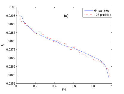
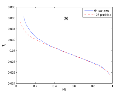
In Fig. 1 we show the temperature distribution on the chain, calculated by both eighth-order Runge-Kutta algorithm [Fig. 1(a)] and velocity Verlet algorithm [Fig. 1(b)]. It is seen from Fig. 1(a) and 1(b) that the linear temperature distribution can be obtained with both algorithms, but there are still some small differences between them. The velocity Verlet algorithm is a very efficient one, by which, a very smooth temperature distribution is obtained, but in this case, the Nosé-Hoover boundary condition on the left end of the chain with higher temperature could not be well treated unless the chain is long enough, which may result from the sensitivity of this algorithm to the thermostat boundary condition. So, we will mainly use the Runge-Kutta algorithm in this work, and the velocity Verlet algorithm is used only as a reference.


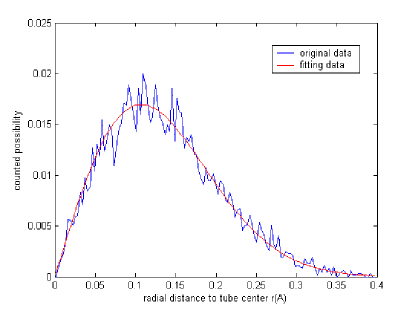
The calculated thermal conductivities of CNWs with different lengths are shown in Fig. 2, in which two types of scales are shown, i.e., linear-log and log-log scale. Here we should explain our definition on the cross section of CNW. The statistical radial distribution for the motion of wire atoms along the direction perpendicular to the tube axis is calculated, and obtained result is given in Fig. 3, which can be fitted by , with the radial distance to the tube axis. It is found that the parameter is equal to 0.151 Å, and so, the final cross section area for the heat transport can be expressed as .
Thus in this case, the thermal conductivity is obtained to be 142 W/mK1323 W/mK, for the chain length from 3 nm to 188 nm, which is very high. For comparison, it is interesting to list the value of the SWNTs with their lengths in the same range, which is about 102 W/mK [20], or about 10103 W/mK [21, 22]. So, the thermal conductivity of CNW is comparable to that of the SWNTs, at least, not much smaller than that of the SWNT. For example, our calculated thermal conductivity of the CNW with 512 atoms is 1.2x10³ W/mK. But Zhang et al. [21] got the corresponding thermal conductivity of nearly 1.6x10³ W/mK for the (5, 5) SWNT having 384 layers (its length is the same as that of the CNW), which is on the same order as our CNW result.
Now, we would like to ask a question: which type of divergence behavior does our CNW system follow? Power law or logarithmic law? From Fig. 2 it is clearly seen that when the system length is increased, the does NOT show completely a linear behavior in both of linear-log and log-log scales, making difficult to justify which type of divergent behavior, power or logarithmic law is suitable to the CNW. But, comparing Fig. 2a with 2b, we could conclude that the of the CNW prefers more the logarithmic divergence than the power law, at least for the middle part of the data from about 32 to 512 atoms, which demonstrates the divergence behavior of the CNW is different from that of the SWNT, following the power law. Why logarithmic for the CNW? We think it is just the transverse motions of the carbon atoms on the CNW to relax its thermal conductance divergence, and lead it to deviate from the 1D power law divergence.
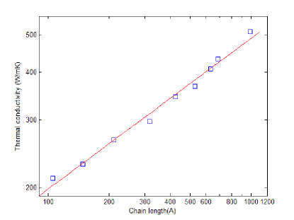
In order to see more clearly the influence of the transverse motion of the CNW, we have also studied the thermal conductivity of perfect 1D carbon chains connected by the Tersoff-Brenner bond order potential, in which, their transverse motions are not permitted. The initial equilibrium distance between their neighboring atoms is set to be 1.65 Å, and their cross sections are determined as follows. As well known, the cutoff distance in the Tersoff-Brenner bond order potential is about 2.0 Å, which can be approximately considered as an interaction range between two nearby carbon chains. So, the cross section of a perfect 1D carbon chain can be roughly estimated to be about 3.14 Å2. The length dependence of the thermal conductivity is shown in Fig. 4. It is seen from Fig. 4 that the diverges with chain length as, , with , and its is about 212 W/m K511 W/m K, which is comparable with the result of CNW.
Comparison between the thermal conductivities of both 1D carbon chain and the quasi-1D CNW clearly show that it is indeed the transverse motions of the carbon atoms on the CNW to cause its logarithmic thermal conductance divergence. We should emphasize that in real systems, the divergence of thermal conductivity will not be as simple as that found in the theoretical models such as FPU model, which probably rests with the aspect ratio of the system.
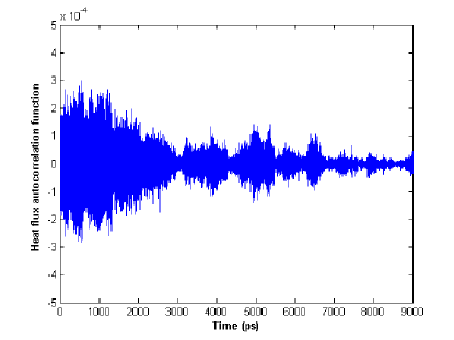
The heat flux autocorrelation function in the case of N=64 is also calculated and shown in Fig. 5, from which it is seen that after a very slow decay in about 9000 ps, the heat flux autocorrelation function decreases to a small value. The similar phenomenon has been observed by Yao et al. [22], which can be understood by the fact that after a long enough evolution, the final state has no relationship with the initial state.
Finally, we will check the validity of ensemble average in this low dimensional system. First, we compare those evolutions starting from the different initial conditions. The obtained results are shown in Fig. 6. Here the low or high initial temperature means the initial temperature of every atom on the chain is set to the lower or higher boundary temperature, respectively. And the linear initial temperature means the initial temperature of every atom is chosen based upon a linear temperature distribution between the two boundaries. All the distributions are calculated after a time interval .
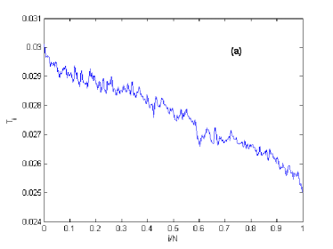
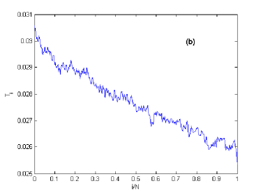
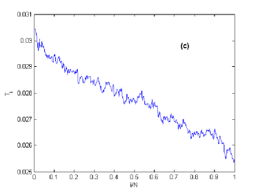
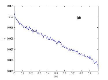
At the first sight, four figures in Fig. 6 seem to be the same. In fact there are only little differences between them, which means our numerical results are reasonable, being independent of the initial conditions. However, it is seen from Fig. 6 that Fig. 6(d) is the smoothest one, which means an average over other three can give a more reliable result, just like averaging over a longer time interval. Thus, we can improve our calculation efficiency by the following method: very different initial states are chosen first, from which the system evolves, and after a period of evolution time, an average over the different system evolutions starting from the different initial conditions can be made. This method can be considered as a high efficient parallel algorithm, by which, the highest acceleration coefficient can be gained.
IV Conclusion
In this paper, the heat conduction of a finite length carbon chain inserted into a (5, 5) SWNT has been studied by using the nonequilibrium molecular dynamics method, in which both longitudinal and transverse motions of the chain atoms are permitted. The interaction between chain atoms and nanotubes has been simulated by a continuous model for the nanotube. It is found that heat conduction of CNW does not obey the Fourier’s law, and its thermal conductivity logarithmicly diverges with CNW length as .
Acknowledgements.
We acknowledge support from the Natural Science Foundation of China under Grants No. 90103038 and No. A040108.References
- (1) C.Giardina, R.Livi, A.Politi, and M.Vassalli, Phys. Rev. Lett. 84, 2144 (2000); S.Lepri, R.Livi, and A.Politi, Phys. Rev. Lett. 78, 1896 (1997).
- (2) B.Hu, B.Li, and H. Zhao, Phys. Rev. E 57, 2992 (1998).
- (3) B.Hu, B.Li, and H. Zhao, Phys. Rev. E 61, 3828 (2000); B.Li, H. Zhao, and B.Hu, Phys. Rev. Lett. 86, 63 (2001); B.Li, L. Wang, and B.Hu, Phys. Rev. Lett. 88, 223901 (2002).
- (4) D.Chen, S.Aubry, and G.P.Tsironis, Phys. Rev. Lett. 77, 4776 (1996).
- (5) D.Alonso, R.Artuso, G.Casati, and I.Guarneri, Phys. Rev. Lett. 82, 1859 (1999).
- (6) S. Lepri, R.Livi, and A.Politi, Europhys. Lett. 43, 271(1998); S.Lepri, R.Livi, and A.Politi, Physica D 119, 140-147 (1998).
- (7) T.Hatano, Phys. Rev. E 59, R1 (1999).
- (8) Ahishek Dhar, Phys. Rev. Lett. 86, 3554 (2001).
- (9) G. Casati and T.Prosen, Phys. Rev. E 67, 015203(R)(2003).
- (10) O.V.Gendelman, A.V.Savin, Phys. Rev. Lett. 84, 2381 (2000); A.V.Savin, G.P.Tsironis, and A.V.Zolotaryuk, Phys. Rev. Lett. 88, 154301 (2002).
- (11) Tbmaz Prosen, and David K. Campbell, Phys. Rev. Lett. 84, 2857 (2000).
- (12) P.L.Garrido, P.I.Hurtado, and B.Nadrowski, Phys. Rev. Lett. 86, 5486 (2001).
- (13) Peter Grassberger and Lei Yang, cond-mat/0204247 (2002).
- (14) Jian-Sheng Wang and Baowen Li, Phys. Rev. Lett. 92, 074302 (2004).
- (15) R.Saito et al., Physical Properties of Carbon Nanotubes (Imperial College Press, London, (1998)
- (16) X. Zhao, Y. Liu, S. Inoue, T. Suzuki, R.O. Jones, and Y. Ando, Phys. Rev. Lett. 92, 125502 (2004)
- (17) J. Hone, M. Whitney, C. Piskoti, and A. Zettl, Phys. Rev. B 59, R2514 (1999)
- (18) P. Kim, L. Shi, A. Majumdar, and P.L. McEuen, Phys. Rev. Lett. 87, 215502 (2001)
- (19) S. Berber, Y.K. Kwon, and D. Tomanek, Phys. Rev. Lett. 84, 4613 (2000)
- (20) Shigeo Maruyama, Physica B 323, 193-195 (2002)
- (21) Gang Zhang and Baowen Li, cond-mat/0403393 (2004)
- (22) Zhenhua Yao, Jian-Sheng Wang, Baowen Li and Gui-Rong Liu, cond-mat/0402616(2004)
- (23) Xinlou Zhao, Yoshinori Ando, Yi Liu, Makoto Jinno, and Tomoko Suzuki, Phys. Rev. Lett. 90, 187401(2003).
- (24) J.Tersoff, Phys. Rev. B 37, 6991 (1988); J.Tersoff, Phys. Rev. Lett. 61, 2879 (1988); Donald W. Brenner, Phys. Rev. B 42, 9458 (1990).
- (25) L. Battezzatti, C. Pisani, F. Ricca, J. Chem. Soc. 71, 1629 (1975).
- (26) L.A. Grrifalco, J. Phys. Chem 96, 858(1992),
- (27) L.A. Girifalco, Phys. Rev. B 52, 9910 (1995).
- (28) K.Kniaz, L.A. Girifalco, and J.E. Fischer, J. Phys. Chem. 99, 16804 (1995).
- (29) K. Kniaz, J.E. Fischer, L.A. Girifalco, A.R. McGhie, R.M. Strongin and A.B. Smith, Solid State Commun. 96, 739 (1995).
- (30) V.I. Zubov, N.P. Tretiakov, J.N. Teixeira Rabelo, and J.F. Sanchez Ortiz, Phys. Lett. A 194, 223 (1994).
- (31) J.P.K. Doye and D. Wales, Chem. Phys. Lett. 247, 339 (1995).
- (32) C. Rey, J. Garcia-Rodeja, L.J. Gallego, J.A. Alonso, Phys. Rev. B 55, 7190 (1997).
- (33) S. Tamaki, N. Ide, I. Okada, and K. Kojima, J. Appl. Phys. 37, 2608 (1998).
- (34) R.S. Ruoff and A.P. Hickman, J. Phys. Chem. 97, 2494 (1993).
- (35) J. Song and R.L. Cappelletti, Phys. Rev. B 50, 14 678 (1994).
- (36) L. Henrard, E. Hernandez, P. Bernier, and A. Rubio, Phys. Rev. B 60, R8521 (1999).
- (37) L.A. Girifalco, Miroslav Hodak, and Roland S. Lee, Phys. Rev. B 62, 13104(2000).
- (38) S.Nosé, J.Chem.Phys. 81, 511 (1984), W.G.Hoover, Phys. Rev. A 31, 1695 (1985)
- (39) M.P. Allen, D.J. Tildesley, Computer Simulation of Liquids, Clarendon Press, Oxford, 1987.
- (40) R. Kubo, M. Toda, and N. Hashitsume, Statistical Physics II, Springer Series in Solid State Sciences Vol. 31 (Springer, Berlin, 1991); A.J.C. Ladd, B.Moran, and W.G. Hoover, Phys. Rev. B 34, 5058 (1986)