Anomalous distribution functions in sheared suspensions

Abstract

We investigate velocity probability distribution functions (PDF) of sheared hard-sphere suspensions. As observed in our Stokes flow simulations and explained by our single-particle theory, these PDFs can show pronounced deviations from a Maxwell-Boltzmann distribution. The PDFs are symmetric around zero velocity and show a Gaussian core and exponential tails over more than six orders of magnitude of probability. Following the excellent agreement of our theory and simulation data, we demonstrate that the distribution functions scale with the shear rate, the particle volume concentration, as well as the fluid viscosity.

Stochastic processes Particle-laden flows Liquids, emulsions, and suspensions; liquid crystals

1 Introduction

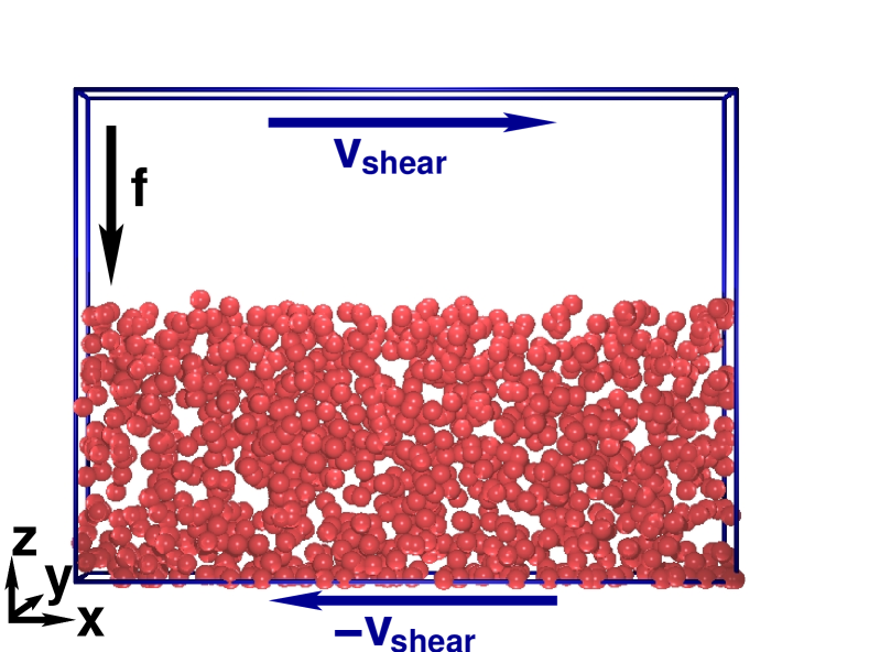
To describe the statistics of complex systems, often probability distribution functions (PDF) are utilized. These distributions have been found to be of non-Gaussian shape in numerous fields of physics, including astrophysics [1], flow in porous media [2], turbulence [3], granular media [4, 5, 6], or suspensions [7, 8, 9]. However, the underlying processes are often not understood. In this letter, we focus on particularly important systems showing non-Gaussian velocity PDFs, namely sedimenting hard-sphere suspensions confined between sheared walls (see Fig. 1). They appear in river beds, blood examinations, industrial food production, the application of paint, and many more situations. Detailed experiments have been performed for more than a hundred years, but questions about the microstructure or structural relaxations of the sediment are still not well understood.

Numerous authors have found that the PDF of particle velocities $P(v)$ is not of similar shape as for an ideal gas, i.e., like a Maxwellian. Instead, $P(v)$ can show a pronounced non-equilibrium shape, where the probability of high velocities is substantially larger [7, 8]. In this letter we present a single-particle theory and simulations to show that such non-equilibrium distributions can be described as a consequence of an irreversible driving process, where particles on average gain energy by one mechanism, but loose energy by another one. Here, energy is gained from the shear or gravitational forces causing particles to collide. Contrarily, energy is dissipated due to viscous damping. This causes $P(v)$ to consist of a Gaussian core and exponential tails. Even though we focus on a well defined system here, the processes described are of general nature and can be applicable to ostensibly different setups.

Experimentally, Rouyer et al. [10] studied quasi 2D hard-sphere suspensions and found a stretched exponential $P(v)$ with concentration dependent exponents between 1 and 2 corresponding to exponential distributions for high concentrations and Gaussians for small particle counts. These results contradict theoretical predictions of a transition from exponential to Gaussian with increasing volume concentration [7, 8]. However, both experimental and theoretical studies do not present sufficient statistics over more than 2-4 decades. It is important to note that if one does not have enough data points for high quality PDFs, final answers on the nature of the function cannot be given. Indeed, in the process of analyzing our data we found that even stretched exponentials can fit PDFs with purely exponential tails and Gaussian centers if only two to four decades of probability are covered. But as soon as more data is added, the exponential nature of the tails becomes distinct and it is impossible to fit the whole PDF with a single function.

Here, we overcome such limitations by presenting PDFs consisting of up to 10¹⁰ particle displacements each – allowing a statistics superior to any previous work. Our data does not show deviations from purely exponential tails over 6-8 decades of probability. We show that $P(v_{z})$ scales linearly with the shear rate, volume concentration and viscosity.

The simulated system is a 3 dimensional setup as shown in Fig. 1. Top and bottom walls are at distance $N_{z}$ and sheared with shear rate $\dot{\gamma}=2v_{\rm shear}/N_{z}$. All other boundaries are periodic. A body force $f$ acting on the otherwise neutrally-buoyant particles can be added to mimic gravity. If turned on, this force causes strong density gradients in the system as can be observed in Fig. 1. We consider 384 to 1728 initially randomly placed suspended particles of equal radius $a$ corresponding to a particle volume concentration $\phi$ between 6.8% and 30.7%. The particle Reynolds number $Re=\dot{\gamma}2a/\nu$ is kept between $0.012$ and $0.07$.

Figure 1: (Color online) Sketch of the simulation setup.

2 Simulation method

The simulation method is composed of a lattice Boltzmann solver (LB) for the fluid and a molecular dynamics (MD) algorithm for the motion of particles. This approach and recent improvements were originally introduced by Ladd and coworkers [11, 12, 13, 14] and are well established in the literature [11, 12, 13, 14, 15, 16]. Thus, we only shortly describe it here.

The LB approach allows to calculate long-range hydrodynamic interactions between particles, by utilizing a discretized version of Boltzmann’s equation [17]. Here, positions $x$ are discretized on a 3D lattice with 19 discrete velocities $c_{i}$ pointing from a site to its neighbors. Every $c_{i}$ is related to a single particle distribution function $f_{i}(x)$ which is streamed to neighboring sites at every time step. After streaming, a collision takes place where the individual $f_{i}(x)$ relax towards an equilibrium distribution $f^{\rm eq}_{i}$. Local mass and momentum density are given by moments of the $f_{i}(x)$. The movement of suspended particles is modeled by Newton’s equation of motion and appropriate boundary conditions are imposed at solid/fluid interfaces to exchange momentum. We find a particle radius of $a$=1.25 lattice sites sufficient since for larger radii $P(v_{z})$ does not change significantly anymore, while the computational effort increases substantially. Also, in low density simulations long-range hydrodynamic interactions dominate which are correctly reproduced even by small particles. For dense systems, exact lubrication forces between particle pairs and between particles and walls are applied [11, 12, 13]. If many particles come close to each other (less than 0.1 lattice spacings), a cluster implicit method is used for updating forces in the MD algorithm [13]. This algorithm does improve the stability of the code and we carefully checked by comparing simulations with different volume concentrations and body forces that it has no influence on the shape of the PDF.

The simulation volume is 64$a$ $\times$ 8$a$ $\times$ 48$a$ and $\dot{\gamma}$ is varied between $2.3\cdot 10^{-4}$ and $1\cdot 10^{-3}$ (in lattice units). The fluid density is kept constant and the kinematic viscosity is set to $\nu=0.05$ if not specified otherwise. A single simulation runs for 6.25 million LB steps, where during the last 5 million steps the $z$ component of the velocity of every particle is gathered in a histogram to obtain $P(v_{z})$. All distributions are normalized such that $\int{\rm d}v_{z}P(v_{z})=1$ and $\int{\rm d}v_{z}v_{z}^{2}P(v_{z})=1$ with the RMS velocity $v_{z}^{\rm RMS}=\sqrt{\langle v_{z}^{2}\rangle}=1$.

3 Theoretical aspects

Our theoretical model is based on the balance between viscous dissipation and shear forcing in steady state. The shear and the resulting particle collisions are modeled by random, diffusive forcing. Due to this forcing, the velocity $v_{j}$ of the $j$th particle changes as $\frac{dv_{j}}{dt}=\xi_{j}$ where $\xi_{j}$ is a white noise, $\langle\xi_{j}\rangle=0$ and $\langle\xi_{i}(t)\xi_{j}(t^{\prime})\rangle=2D\delta_{ij}\delta(t-t^{\prime})$. In parallel, particles slow down because of the viscous fluid. In accordance with the traditional drag law, the velocity decreases according to $dv/dt=-\beta v$, resulting in the exponential decay $v(t)=v(0)e^{-\beta t}$ in the absence of forcing. We model this viscous damping by reducing each time unit $\Delta t$ the velocity by a factor $\eta=e^{-\beta}\Delta t$ according to $v\to\eta v$. In a sheared fluid, there is a well defined time scale for re-encounters with the boundary, setting the time scale for the damping process. This damping process was used by van Zon et al. as a model for forced granular media [18, 19].

The velocity distribution obeys the linear but non-local equation

$$\frac{\partial P(v)}{\partial t}=D\frac{\partial^{2}P(v)}{\partial^{2}v}+\frac{1}{\eta}P\left(\frac{v}{\eta}\right)-P(v)\mbox{.}$$ (1)

The first term on the right hand side represents changes due to diffusive forcing and the next two terms represent changes due to viscous damping. In our theory, interactions between particles are represented through the random forcing process reflecting that a particle undergoes diffusion as influenced by all other particles. In steady state, the left hand side of Eq. 1 vanishes. We note that the shape of $P(v)$ is independent of the diffusion constant $D$. Indeed, by making the scaling transformation $v\rightarrow v/\sqrt{D}$ we can eliminate $D$ and assume without loss of generality that $D=1$. The shape of the distribution depends on the dissipation parameter $\eta$ alone. The moments

$$M_{n}=\int dv\,v^{n}P(v)$$ (2)

satisfy the recursion relation

$$M_{n}={n(n-1)}(1-\eta^{n})^{-1}M_{n-2}.$$ (3)

Since the distribution is symmetric, $P(v)=P(-v)$, the odd moments vanish and starting with $M_{0}=1$, the even moments are

$$M_{2n}=(2n)!\prod_{k=1}^{n}\frac{1}{1-\eta^{2k}}\mbox{.}$$ (4)

Of particular interest is the normalized 4th moment

$$\kappa=M_{4}/M_{2}^{2}={6}/(1+\eta^{2}).$$ (5)

The distribution is close to exponential for strong drag, $\kappa\to 6$ as $\eta\to 0$ and close to Gaussian for very weak drag, $\kappa\to 3$ as $\eta\to 1$. This is confirmed by the limiting behaviors of all moments

$$M_{2n}\to\left\{\begin{array}[]{l@{\quad\eta\to\,}l}(2n)!&0\mbox{,}\\ (2n-1)!!(1-\eta)^{-n}&1\mbox{.}\end{array}\right.$$ (6)

The leading large-velocity behavior can be derived by using a heuristic argument. For sufficiently large velocities, the term $\eta^{-1}P\left(v\eta^{-1}\right)$ is negligible and hence,

$$\frac{d^{2}}{dv^{2}}P(v)=P(v).$$ (7)

Thus, $P(v)$ has an exponential tail, $P(v)\sim\exp\big{(}-|v|\big{)}$. The prefactor can be obtained from the Fourier transform $F(k)$ that equals an infinite series

$$F(k)=\int_{0}^{\infty}dve^{ikv}P(v)=\prod_{m=0}^{\infty}[1+k^{2}\eta^{2m}]^{-1}.$$ (8)

This expression follows from the steady-state analog of (1), $(1+k^{2})F(k)=F(\eta k)$. The simple poles at $\pm i$ closest to the origin imply an exponential decay, i.e.,

$$P(v)\simeq{A(\eta)}\exp(-{|v|}),$$ (9)

when $|v|\to\infty$. Re-summation yields the residue to this pole, and in turn, the prefactor

$$A(\eta)=\frac{1}{2}\exp\left(\sum_{n=1}^{\infty}\frac{1}{n}\frac{\eta^{2n}}{1-\eta^{2n}}\right).$$ (10)

The exponential behavior is robust in the limit $v\to\infty$. However, in the weak drag limit, $\eta\to 1$, the exponential behavior holds only for extremely large velocities. When $\eta\to 1$, ($\eta=1-\varepsilon,\varepsilon\to 0$) we expand the denominator in $A(\eta)$. Keeping only the dominant terms simplifies the sum to

$$\sum_{n=1}^{\infty}\frac{1}{2\varepsilon n^{2}}=\frac{\pi^{2}}{12\varepsilon}$$ (11)

and to leading order, the prefactor is $A\propto\frac{1}{2}\exp\left[\pi^{2}/12\varepsilon\right]$. Therefore, under weak damping, there is a cross-over between a Maxwellian behavior as follows from (6) and an exponential one,

$$P(v)\sim\left\{\begin{array}[]{@{\,}l@{\quad v\,}c@{\,\epsilon^{-1}}l}\exp\left(-\frac{\varepsilon v^{2}}{2}\right)&\ll\hfil\,\varepsilon&\mbox{,}\\ \exp\left(\frac{\pi^{2}}{12\varepsilon}-|v|\right)&\gg\hfil\,\varepsilon&\mbox{.}\end{array}\right.$$ (12)

The two expressions match $P(v)\sim\exp\big{(}-\varepsilon^{-1}\big{)}$ at the crossover velocity $v\approx\varepsilon^{-1}$. Interestingly, the crossover to a non-Maxwellian does not affect the leading behavior of the moments.

In summary, the theory predicts the non-equilibrium shape of the PDF as an interplay between energy being injected by a diffusive thermostat and dissipation due to the fluid drag. In general, the high-velocity tail is exponential. The theoretical results shown later in this letter are given by a Monte Carlo solution of the steady state case of Eq. 1. In these simulations, $N$ particles are characterized by a velocity $v_{i}$. The velocities change through two independent processes: damping and random forcing. In the damping process, the velocity is reduced by a fixed factor $v_{i}\to\eta v_{i}$. In the forcing process, the particle velocity changes by a random increment $v_{i}\to v_{i}+\xi$ where $\xi$ has zero mean and a unit variance. The steady-state distributions were obtained using over $10^{10}$ points from simulations with $10^{8}$ particles.

4 Results

Figure 2: (Color online) $P(v_{z})$ for $f=0.72\cdot 10^{-4}$ corresponding to a Stokes velocity of $v_{s}$=$1.4\cdot 10^{-3}$, $\phi=13.6\%$ and shear rates $3.3\cdot 10^{-4}$, $6.7\cdot 10^{-4}$, and $1\cdot 10^{-3}$ ($Re$=$0.017$, $0.034$, $0.05$). The solid line is the steady state solution of Eq. 1 ($\eta=0.73$). The lower inset shows the unscaled data, where higher $\dot{\gamma}$ relate to wider $P(v_{z})$. The upper inset shows a linear fit with slope 0.21 of $v_{z}^{\rm RMS}(\dot{\gamma})$ for the PDFs presented in the main figure as well as four additional datasets (symbols).

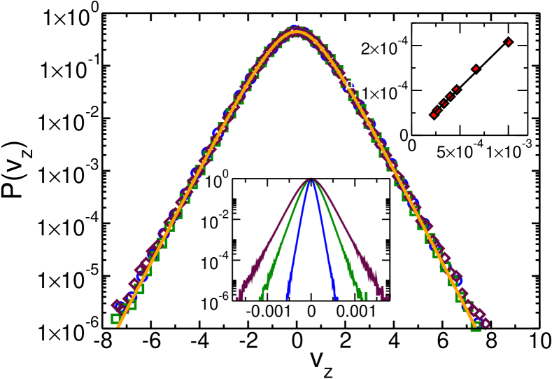
First, we consider suspensions with constant $\phi$ and various shear rates under the influence of a body force $f$. The dependence of $P(v_{z})$ on $\dot{\gamma}$ for three representative values is depicted in Fig. 2. $P(v_{z})$ is symmetric and $\langle v_{z}\rangle=0$ for all cases considered in this letter. As shown in the lower inset, the not normalized $P(v_{z})$ widen for higher $\dot{\gamma}$. However, a very good scaling is observed: all normalized curves collapse onto a single one. In the upper inset we show the influence of $\dot{\gamma}$ on $v_{z}^{\rm RMS}$: as expected from the theory, $\dot{\gamma}$ only sets a scale for the velocity corresponding to a linear relation between $\dot{\gamma}$ and $v_{z}^{\rm RMS}$. $P(v_{x})$ (after deducting the shear velocity) and $P(v_{y})$ also show Gaussian cores and exponential tails, although their width and height are different. Thus, the general shape of distributions in different directions is essentially identical and they are therefore not shown. To obtain an insight into the properties of $P(v_{z})$, we compute the cumulant $\kappa$ and find that for all simulation parameters studied in this letter it varies between 3.8 and 4.6. Knowing $\kappa$, we can compute $\eta=\sqrt{6/\kappa-1}$. Due to the large number of data points in our histograms, we calculate $\kappa$ for periods of 1 million time steps each and use the arithmetic average of the last 5 million time steps of a simulation run. We find that $\kappa$ varies by up to 10% within a single simulation which is of the same order as the difference of the individual PDFs in Fig. 2. Thus, we average the different curves as well in order to obtain a value for the cumulant to be utilized for the Monte Carlo solution of the steady state case of Eq. 1. For the collapse in Fig. 2 we get $\eta=0.73$. As depicted here, the solid line given by the theory and the simulation data excellently agree over the full range of six decades of probability.

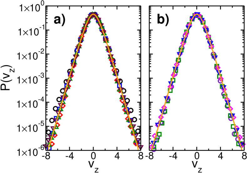
Next, we consider neutrally-buoyant suspended hard spheres ($f=0$)under shear. The shear rate is kept fixed and the particle concentration is varied between $\phi=6.8\%$ and $30.7\%$. Due to hydrodynamic interactions, the particles tend to move to the center of the system, i.e., to an area where the shear is low creating a depleted region close to the walls. However, this effect does not change the general shape of $P(v)$. The corresponding normalized $P(v_{z})$ are presented in Fig. 3a.

Figure 3: (Color online) $P(v_{z})$ for $f=0$, $\dot{\gamma}=6.7\cdot 10^{-4}$ and $\phi=6.8\%,13.6\%,20.5\%,23.9\%$, and $27.3\%$, $Re=0.034$ (a). In Fig. b), $\phi$ is kept at $13.6\%$ and the kinematic viscosity is set to $\nu=0.017$, $0.05$, and $0.1$ ($Re=0.099$, $0.034$, $0.067$). In both figures, all data sets collapse onto a single curve and the lines are given by the theory with $\eta=0.69$.

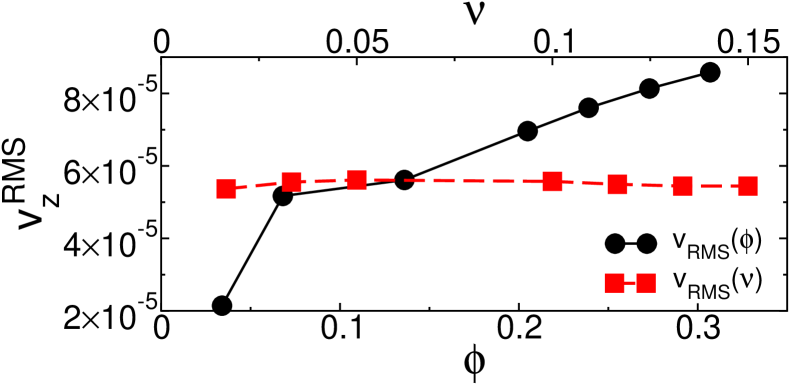
As depicted in the figure, all PDFs except for the lowest particle concentration $\phi=6.8\%$ (circles) collapse onto a single curve. At very low $\phi$, the tails of $P(v_{z})$ are still not fully converged due to the limited number of particle-particle interactions taking place within the simulation time frame. Again, the solid line in Fig. 3a is given by the steady state solution of Eq. 1 with $\eta=0.69$ being obtained from the 4th moment of $P(v_{z})$. As before, simulation and theory agree very well. The full circles in Fig. 4 depict the dependence of $v_{z}^{\rm RMS}$ on $\phi$. For concentrations of at least $\phi=13.6\%$, $v_{z}^{\rm RMS}(\phi)$ can be fitted by a line with slope $1.8\cdot 10^{-4}$. The disagreement of the linear fit for low $\phi$ is consistent with the not fully converged PDFs as shown in Fig. 3a. By keeping all parameters except the kinematic viscosity $\nu$ constant, the dependence of $\nu$ on $P(v_{z})$ can be studied. As demonstrated by the squares depicting the dependence of $v_{z}^{\rm RMS}$ on $\nu$ in Fig. 4, $v_{z}^{\rm RMS}$ and thus $P(v_{z})$ is independent of the viscosity. Thus, the steady state curve obtained for different volume concentrations is identical to the one for different $\nu$ as shown in Fig. 3b.

Figure 4: (Color online) $v_{z}^{\rm RMS}$ in dependence of $\phi$ (circles) and $\nu$ (squares). Data corresponds to $P(v_{z})$ as in Fig. 3, but covers a wider range of $\phi$ and $\nu$. Note the different $x$-axes.

It would be interesting to study the influence of the body force $f$ on the shape of the PDF. However, $f$ and the shear forces are in a subtle interplay since the height of the steady state sediment depends on both parameters and thus influences the local concentration. To investigate this behavior is beyond the scope of this letter.

5 Conclusion

To conclude, the non-equilibrium PDFs reported in this letter are a consequence of the irreversible nature of the driving process. On average, particles gain energy by external forces causing particle-particle collisions but lose energy by viscous damping. Unlike in an ideal gas, these two mechanisms are not interchangeable. In other words, one cannot reverse the arrow of time and observe the same behavior. Our theoretical model captures this irreversibility through the competition between two non-equivalent driving mechanisms: energy dissipation through a multiplicative process and energy injection through an ordinary additive diffusive thermostat.

The theory describes all aspects of the distribution as demonstrated by an excellent agreement with our coupled LB/MD simulations of sheared suspensions: the velocity distribution functions $P(v_{z})$ exhibit Gaussian cores and exponential tails over at least 6 orders of magnitude of probability. This finding is consistent with experimental results as given for example in [4]. We also note that the complete shape of the distribution can be characterized by a single parameter, the normalized 4th moment that has a one to one correspondence with the theoretical dissipation parameter. Further, we confirmed that $P(v_{z})$ scales linearly with the particle volume concentration as well as the shear rate and is independent on the solvent’s viscosity.

While various authors report on transitions between Gaussian and (stretched) exponential tails [7, 8, 10], our results do not confirm such transitions. A likely reason for the previously published results might be the lack of sufficient statistics. If only two to four orders of magnitude of probability are covered, $P(v_{z})$ can be reasonably well fitted by pure Gaussians or distributions with (stretched) exponential tails as well. For a conclusive answer on the shape of the PDF, we found that at least five to six orders of magnitude of probability and a proper normalization are necessary. Experiments in strongly driven granular particles suspended in a fluid provide evidence of exponential velocity distributions [4]. In order to close the question of the general validity of the findings presented in this letter, further high quality experimental or numerical data would be needed.