Renormalization of Singular Potentials and Power Counting

Abstract

We use a toy model to illustrate how to build effective theories for singular potentials. We consider a central attractive $1/r^{2}$ potential perturbed by a $1/r^{4}$ correction. The power-counting rule, an important ingredient of effective theory, is established by seeking the minimum set of short-range counterterms that renormalize the scattering amplitude. We show that leading-order counterterms are needed in all partial waves where the potential overcomes the centrifugal barrier, and that the additional counterterms at next-to-leading order are the ones expected on the basis of dimensional analysis.

I Introduction

Singular potentials —those that diverge as $1/r^{n}$, $n\geq 2$ at a small distance $r$— are common in atomic, molecular and nuclear physics frank_land_spector . Contrary to the regular case, a sufficiently attractive singular potential does not determine observables uniquely case . A proper formulation of the extra ingredients can be found in the framework of effective field theory (EFT) beane , where the problem is cast in the usual language of renormalization. With the techniques of renormalization one retains the predictive power of singular potentials at low energies, while short-distance physics is accounted for in a minimal, model-independent way.

The basic idea is that in order to obtain the potential from some underlying theory we make an arbitrary decomposition between short- and long-distance physics through a short-distance cutoff $R\sim 1/\Lambda$, above which the potential has a form determined by the exchange of light particles —such as two-photon exchange in the case of van der Waals forces, or pion exchange in nuclear physics. When the long-range potential is regular, or singular and repulsive, the quantum-mechanical dynamics is insensitive to $R$. When the potential is singular and attractive, on the other hand, observables would depend sensitively on $R$ if we ignored short-distance physics. Dependence on the arbitrary scale $R$ can be removed beane by adjusting parameters of the potential at short distances as functions of $R$ (“running constants”) to guarantee that low-energy observables are reproduced independently of $R$. Such short-range “counterterms” are thus used to mimic the effects of short-distance physics.

The case of the $S$ wave in an attractive singular central potential $1/r^{n}$ was considered in Ref. beane , and the particular cases $n=2$ and $n=4$ were studied in more detail in Refs. coon ; hammer and mary , respectively. It was shown that a single counterterm —for example, in the form of the depth of a square-well— is sufficient to ensure an approximate $R$ independence of low-energy observables, once one observable is used to determine the running of the counterterm. An interesting property of this running, first noticed in the three-body system 3bozos , is an oscillatory behavior characteristic of limit cycles. For example, when $n=2$ the short-distance force has a fixed period as a function of $\ln R$. Limit cycles are now a subject of renewed interest limits .

A consistent EFT must in addition provide systematic improvement over this simple picture. If we consider particles of typical momentum $Q$, we would like to be able to calculate observables in an expansion in powers of $QR_{sh}=Q/M_{hi}$, where $R_{sh}\equiv 1/M_{hi}$ is the range of short-range physics. Successive terms in this expansion are referred to as leading order (LO), next-to-leading order (NLO), and so on. Determining at which orders interactions contribute is called “power counting”.

We are interested here in a two-body system in a regime of momenta where LO comes from a dominant long-range potential that is attractive and singular, together with the required counterterms. The latter include one $S$-wave counterterm beane . However, the long-range potential contributes also to other partial waves, and it has been argued on general terms behncke68 that counterterms are required in those waves as well. In the particular case of nucleons, one-pion exchange has an $1/r^{3}$ tensor force in spin-triplet channels; it has been shown explicitly that counterterms are necessary in all waves where the tensor force is attractive and iterated to all orders towards ; nogga_timmermans_vankolck ; spaniards1 . (For a different point of view, see Ref. germans .) This poses a potential problem because predictive power seems to be lost in systems with more than two particles, where all two-particle waves contribute. In Ref. nogga_timmermans_vankolck a solution was proposed where, thanks to the centrifugal barrier, perturbation theory in the long-range potential is employed in waves of sufficiently large angular momentum. We would like to better understand the role of angular momentum, and establish the number of short-range counterterms needed in LO to make sense of a singular potential.

In general a dominant long-range potential suffers corrections that increase as the distance decreases. These corrections can arise from additional, smaller couplings to the light exchanged particles —e.g. magnetic photon couplings of the Pauli type. They can also be generated by the simultaneous exchange of several light particles —such as two-pion exchange. These effects lead to potentials that fall faster at large distances than the LO potential. For example, an LO $1/r^{n}$ potential might have an NLO correction $R_{sh}^{2}/r^{n+2}$, as is the case for two-pion exchange between nucleons, which (neglecting nucleon excitations) goes weinberg ; others ; sameold as $R_{sh}^{2}/r^{5}$ with $R_{sh}=(4\pi f_{\pi})^{-1}\simeq 0.2$ fm the characteristic QCD scale. These potentials, which are subleading at distances $r\hskip 1.99997pt\raisebox{2.15277pt}{$>$}\raisebox{-3.00003pt}{$\sim$}\hskip 1.99997ptR_{sh}$, are more singular than the LO potential and overcome it for $r\hskip 1.99997pt\raisebox{2.15277pt}{$<$}\raisebox{-3.00003pt}{$\sim$}\hskip 1.99997ptR_{sh}$. The enhanced singularity ought to demand new counterterms. The desired expansion in $QR_{sh}$ requires that NLO counterterms, which represent physics at $r\hskip 1.99997pt\raisebox{2.15277pt}{$<$}\raisebox{-3.00003pt}{$\sim$}\hskip 1.99997ptR_{sh}$, balance the NLO long-range potential —that is, the full NLO should be such that changes in observables are small. If that is the case, we expect towards that one can treat the NLO potential in perturbation theory. One would also expect nogga_timmermans_vankolck the number of counterterms to be given by naive dimensional analysis —for example, that an NLO correction $R_{sh}^{2}/r^{n+2}$ needs counterterms with two more derivatives than the counterterms required by the LO $1/r^{n}$. In the nuclear case, existing calculations have followed sameold instead the original suggestion weinberg that subleading corrections in the potential be iterated to all orders. In fact, it has been argued spaniards2 that this requires fewer counterterms than doing perturbation theory on the corrections. Nevertheless, treating small corrections in perturbation theory is conceptually simpler, as the running of the LO counterterms is not completely modified by the higher singularity of the NLO potential. Understanding the strengths and limitations of a perturbative approach would at the very least help delineate the scope of a resummation of NLO corrections.

In this paper we address the issue of power counting for singular potentials, in particular the role of centrifugal forces in LO and the perturbative renormalizability of NLO interactions. We examine this issue in a simple toy model, where the LO and NLO long-range potentials are taken as (central) $-1/r^{2}$ and $\pm 1/r^{4}$, respectively. Some of our arguments are similar to those employed in related two coverass2 and three coverass3 ; nnlodispute ; birse -body contexts. We show that LO counterterms are required in all partial waves up to a critical value, and that the number of NLO counterterms is just what is expected on the basis of dimensional analysis. Most of our conclusions can be extended to other attractive singular potentials.

This paper is organized as follows. In Sect. II we discuss our EFT framework. In Sect. III a new approach for treating the $-1/r^{2}$ potential is presented. In Sect. IV the renormalization of the NLO amplitude is discussed and, as a result, NLO counterterms are found. We discuss some of the implications of our results to other potentials in Sect. V. Finally, we summarize our findings in Sect. VI.

II Framework

We consider two non-relativistic particles of reduced mass $m$ in the center-of-mass frame, which interact through a potential $V$. Our analysis will mainly be based upon the Lippmann-Schwinger equation of the half-off-shell $T$ matrix,

$$T({\bm{p}}^{\prime},{\bm{p}})=V({\bm{p}}^{\prime},{\bm{p}})+2m\int\frac{d^{3}q}{(2\pi)^{3}}\frac{V({\bm{p}}^{\prime},{\bm{q}})}{p^{2}-q^{2}+i\epsilon}T({\bm{q}},{\bm{p}})\,,$$ (1)

where ${\bm{p}}$ (${\bm{p}}^{\prime}$) is the initial (final) -state relative momentum. The physics of angular momentum is most transparent when we use a partial-wave decomposition. Our convention is that a quantity $O$ is given in terms of its partial-wave projection $O_{l}$ by

$$O({\bm{p}}^{\prime},{\bm{p}})=\sum_{l=0}^{\infty}(2l+1)O_{l}(p^{\prime},p)P_{l}(\cos\theta)\,,$$ (2)

where $\theta$ is the angle between ${\bm{p}}$ and ${\bm{p}}^{\prime}$. The partial-wave version of Eq. (1) is

$$T_{l}(p^{\prime},p) = V_{l}(p^{\prime},p)-\frac{m}{\pi^{2}}\int_{0}^{\Lambda}dq\frac{q^{2}}{q^{2}-p^{2}-i\epsilon}V_{l}(p^{\prime},q)T_{l}(q,p)\,.$$ (3)

Here we have inserted the ultraviolet cutoff $\Lambda$, which is in general needed to obtain a well-defined solution. Since $\Lambda$ is arbitrary, observables (obtained from the on-shell $T$ matrix) should be independent of $\Lambda$,

$$\Lambda\frac{d}{d\Lambda}T\left(p,p\right)=0\;,$$ (4)

that is, renormalization-group (RG) invariant. It proves convenient to introduce the reduced partial amplitude

$$t_{l}(p^{\prime},p)\equiv\frac{mp}{\pi^{2}}T_{l}(p^{\prime},p)\,,$$ (5)

in terms of which Eq. (3) becomes

$$t_{l}(p^{\prime},p) = \frac{mp}{\pi^{2}}V_{l}(p^{\prime},p)-\int_{0}^{\Lambda}dq\frac{q}{q^{2}-p^{2}-i\epsilon}\frac{mq}{\pi^{2}}V_{l}(p^{\prime},q)t_{l}(q,p)\,.$$ (6)

We will also use in numerics the $K$ matrix because of its reality. The $K$ matrix satisfies the same integral equation as $T$ but with $i\epsilon$ replaced by the principal-value prescription. The reduced form for the partial-wave-projected $K$ matrix,

$$k_{l}(p^{\prime},p)\equiv\frac{mp}{\pi^{2}}K_{l}(p^{\prime},p)\,,$$ (7)

satisfies

$$k_{l}(p^{\prime},p)=\frac{mp}{\pi^{2}}V_{l}(p^{\prime},p)-\mathscr{P}\int_{0}^{\Lambda}dq\frac{q}{q^{2}-p^{2}}\frac{mq}{\pi^{2}}V_{l}(p^{\prime},q)k_{l}(q,p)\,.$$ (8)

The on-shell $k_{l}(p,p)$ is related to $l$-wave phase shift $\delta_{l}(p)$ by

$$k_{l}(p,p)\equiv\frac{\tan\delta_{l}(p)}{\pi^{2}}\,.$$ (9)

We assume a simple central potential, whose dominant long-range component is singular and attractive. We write the potential as

$$V({\bm{p}}^{\prime},{\bm{p}})=V_{L}({\bm{p}}^{\prime},{\bm{p}})+V_{S}({\bm{p}}^{\prime},{\bm{p}})$$ (10)

in terms of a long-range component $V_{L}$ and a short-range component $V_{S}$. The short-range component $V_{S}(r)$ is a series of derivatives of delta functions, so $V_{S}({\bm{p}}^{\prime},{\bm{p}})$ is a power series in ${\bm{p}}^{2}$, ${\bm{p}}^{\prime 2}$, and ${\bm{p}}\cdot{\bm{p}}^{\prime}$, starting with a constant. For definiteness, we take the long-range component to be

$$V_{L}(r)=V_{L}^{(0)}(r)+V_{L}^{(1)}(r)\,.$$ (11)

Here $V_{L}^{(0)}(r)$ is an attractive inverse-square potential,

$$V_{L}^{(0)}(r)=-\frac{\lambda}{2mr^{2}}\,,$$ (12)

with $\lambda>0$ a dimensionless parameter. Its Fourier transform is

$$V_{L}^{(0)}({\bm{p}}^{\prime},{\bm{p}})=-\frac{\pi^{2}\lambda}{m|{\bm{p}}^{\prime}-{\bm{p}}|}\,,$$ (13)

and its partial-wave projection,

$$V_{L\,l}^{(0)}(p^{\prime},p)=-\frac{\pi^{2}\lambda}{m\,(2l+1)}\,\left[\theta(p^{\prime}-p)\,\frac{p^{l}}{p^{\prime l+1}}+\theta(p-p^{\prime})\,\frac{p^{\prime l}}{p^{l+1}}\right]=-\frac{\pi^{2}\lambda}{m\,(2l+1)}\,\frac{p_{<}^{l}}{p_{>}^{l+1}}\,,$$ (14)

where $p_{>}\equiv\max\{p^{\prime},p\}$ and $p_{<}\equiv\min\{p^{\prime},p\}$. In addition, $V_{L}^{(1)}(r)$ is an inverse-quartic potential,

$$V_{L}^{(1)}(r)=-\frac{g}{2mM^{2}r^{4}}\,,$$ (15)

with $M$ a mass scale and $g$ another dimensionless parameter. $V_{L}^{(1)}$ is more singular than $V_{L}^{(0)}$, which in momentum space is reflected in higher powers of momenta in the numerator. To define the Fourier transform we need to limit the integration to distances larger than a coordinate-space cutoff $R$:

$$V_{L\,l}^{(1)}(p^{\prime},p;R) = 4\pi\int_{R}^{\infty}drr^{2}j_{l}(p^{\prime}r)V^{(1)}(r)j_{l}(pr)$$ (16)

$$= -\frac{\pi^{2}g}{2mM^{2}}\left\{\frac{4}{\pi R}\delta_{l0}+\frac{1}{(2l+1)(2l-1)}\frac{p_{<}^{l}}{p_{>}^{l-1}}\left(1-\frac{2l-1}{2l+3}\frac{p_{<}^{2}}{p_{>}^{2}}\right)+O\left(Rp_{>}^{2}\right)\right\}\,.$$

The first term is a constant and cannot be separated from an $S$-wave short-range interaction; it can therefore be absorbed in $V_{S}$, and we drop it not to clutter notation. In the limit $R\to 0$, one is then left with

$$V_{L\,l}^{(1)}(p^{\prime},p)=-\frac{\pi^{2}g}{2mM^{2}}\frac{1}{(2l+1)(2l-1)}\frac{p_{<}^{l}}{p_{>}^{l-1}}\left(1-\frac{2l-1}{2l+3}\frac{p_{<}^{2}}{p_{>}^{2}}\right)\,.$$ (17)

We take $M$ to be the characteristic scale of the underlying theory, $M=M_{hi}$, and $|g|\sim\lambda$. In this case, $V_{L}^{(1)}$ is a correction to $V_{L}^{(0)}$ at large distances $r\hskip 1.99997pt\raisebox{2.15277pt}{$>$}\raisebox{-3.00003pt}{$\sim$}\hskip 1.99997pt1/M_{hi}$ or, equivalently, small momenta $p_{>}\hskip 1.99997pt\raisebox{2.15277pt}{$<$}\raisebox{-3.00003pt}{$\sim$}\hskip 1.99997ptM_{hi}$. We want the short-range component $V_{S}$ to be such that an expansion in $Q/M_{hi}$ holds for observables obtained from the $T$ (or $K$) matrix. Accordingly, we split $V_{S}$, $T$ and $K$ as in Eq. (11) with the superscript ⁽⁰⁾ (⁽¹⁾) denoting LO (NLO). RG invariance is exact only if all orders are considered. Once a truncation to a finite order is made, Eq. (4) can only be satisfied up to terms that vanish as $\Lambda\to\infty$ and can be absorbed in higher-order counterterms. In the rest of the paper we address the question of which terms should be included in the short-range potential at each order to ensure a perturbative expansion of observables consistent with RG invariance.

III $-1/r^{2}$ as LO long-range potential

We first tackle the problem in LO, that is, we take $V_{L}^{(1)}=0$. The $S$-wave renormalization of an attractive inverse-square potential, $-1/r^{2}$, has been dealt with in coordinate- and momentum-space in Refs. beane ; coon and hammer , respectively. Here we present a new approach in momentum space, for any partial wave $l$. Our $l=0$ results reproduce known results beane ; coon ; hammer .

III.1 Singularity of $-1/r^{2}$

To see the origin of the peculiarities of a singular potential, we start by taking $V_{S}^{(0)}=0$. In this case we can write the integral Eq. (6) in a simplified form

$$t_{l}(px,p) = -\frac{\lambda}{2l+1}\,\left\{x^{-(l+1)}\left[\theta(x-1)\,-\int_{0}^{x}dy\frac{y^{l+2}}{y^{2}-1-i\epsilon}t_{l}(py,p)\right]\right.$$ (18)

$$\left.\qquad\qquad+x^{l}\left[\theta(1-x)\,-\int_{x}^{\Lambda/p}dy\frac{y^{1-l}}{y^{2}-1-i\epsilon}t_{l}(py,p)\right]\right\}\,.$$

In this form, we see that the only dimensionful parameter is $\Lambda$, and scale invariance is evident in the limit $\Lambda\to\infty$ (if it existed).

The validity of a perturbative expansion in powers of $\lambda$ can be estimated by comparing the first two terms,

$$-\frac{\lambda}{2l+1}$$ (19)

and

$$-\frac{\lambda^{2}}{(2l+1)^{2}}\left(\frac{1}{2l+1}+i\frac{\pi}{2}\right)\,,$$ (20)

in the expansion of the on-shell $t_{l}(p,p)$ in Eq. (18). We see that perturbation theory in $\lambda$ works well when $l$ is high enough. Conversely, if

$$l\hskip 1.99997pt\raisebox{2.15277pt}{$<$}\raisebox{-3.00003pt}{$\sim$}\hskip 1.99997ptl_{p}\equiv\frac{\lambda\pi}{4}-\frac{1}{2}\,,$$ (21)

Eq. (3) has to be solved for non-perturbatively. The LO amplitude $T^{(0)}$ is in this case obtained from an exact solution of Eq. (3) with the LO potential, as shown diagrammatically in Fig. 1.

Figure 1: LO amplitude $T^{(0)}$ as an iteration of the LO potential $V^{(0)}$.

In order to study the non-perturbative regime, we note that the inverse-square potential, Eq. (13), has the interesting property

$$-{{\bm{\nabla}}^{\prime}}^{2}V_{L}^{(0)}({\bm{p}^{\prime}},{\bm{p}})=-\frac{\lambda}{2m}(2\pi)^{3}\delta^{3}({\bm{p}^{\prime}}-{\bm{p}})\,,$$ (22)

where ${\bm{\nabla}}^{\prime}\equiv\frac{\partial}{\partial{\bm{p}}^{\prime}}$. Using this property we can convert the Lippmann-Schwinger equation, Eq. (1), into a differential equation,

$${{\bm{\nabla}}^{\prime}}^{2}T({\bm{p}}^{\prime},{\bm{p}})+\frac{\lambda}{p^{\prime 2}-p^{2}-i\epsilon}T({\bm{p}}^{\prime},{\bm{p}})=\frac{4\pi^{3}\lambda}{m}\delta^{3}({\bm{p}}^{\prime}-{\bm{p}})\,,$$ (23)

or, decomposed onto partial waves,

$$x\frac{\partial^{2}}{\partial{x}^{2}}\left(xt_{l}(px,p)\right)+\left[\frac{\lambda x^{2}}{{x}^{2}-1-i\epsilon}-l(l+1)\right]t_{l}(px,p)=\lambda\,\delta(1-x)\,.$$ (24)

Treating $p$ as a parameter, let us consider the solution of Eq. (24). If $t_{l}(0,p)$ is assumed finite, which can be inferred from the integral equation, then $t_{l}(px,p)$ for $x<1$ is determined up to a coefficient that is a function of $p$,

$$t_{l}(px,p)=\mathcal{N}_{l}(p/\Lambda)\,x^{l}\;{{}_{2}F_{1}}\left(\frac{1}{2}\left(l+\frac{1}{2}-i\nu_{l}\right),\frac{1}{2}\left(l+\frac{1}{2}+i\nu_{l}\right),\frac{3}{2}+l;x^{2}\right)\,,$$ (25)

where ${{}_{2}F_{1}}(\alpha,\beta,\gamma;z)$ is a hypergeometric function, and

$$\nu_{l}=\sqrt{\lambda-(l+1/2)^{2}}\,.$$ (26)

The pre-factor $\mathcal{N}_{l}$ must be a function of $p/\Lambda$ on dimensional grounds. It is necessary for calculating the on-shell $t_{l}(p,p)$. When $x>1$, the solution is the linear combination of two generic solutions,

$$t_{l}(px,p) = A_{l}(p/\Lambda)\,x^{l}\;{{}_{2}F_{1}}\left(\frac{1}{2}\left(l+\frac{1}{2}-i\nu_{l}\right),\frac{1}{2}\left(l+\frac{1}{2}+i\nu_{l}\right),\frac{3}{2}+l;x^{2}\right)$$ (27)

$$+B_{l}(p/\Lambda)\,x^{-l-1}\;{{}_{2}F_{1}}\left(-\frac{1}{2}\left(l+\frac{1}{2}+i\nu_{l}\right),-\frac{1}{2}\left(l+\frac{1}{2}-i\nu_{l}\right),\frac{1}{2}-l;x^{2}\right)$$

with coefficients $A_{l}$ and $B_{l}$ that can also be functions of $p/\Lambda$. Since Eq. (24) is inhomogeneous only at $x=1$, there is no way to obtain $\mathcal{N}_{l}$ unless we determine the ratio of $A_{l}$ to $B_{l}$ and then match to Eq. (25). This matching brings cutoff dependence to $\mathcal{N}_{l}$. If the $x>1$ solution were cutoff independent (up to $O(p^{2}/\Lambda^{2})$ corrections), one could expect $\mathcal{N}_{l}$ and thus $t_{l}(p,p)$ to be constant, independent of $p$ —a consequence of scale invariance.

The $x>1$ solution simplifies in the asymptotic region. For $x\gg 1$, Eq. (24) becomes

$$x\frac{\partial^{2}}{\partial{x}^{2}}(xt_{l}(px,p))+\left[\lambda-l(l+1)\right]t_{l}(px,p)=O\left(\frac{t_{l}}{{x}^{2}}\right)\,.$$ (28)

This equation has two generic solutions,

$$t_{l}(px,p)\propto x^{\,\left(-\frac{1}{2}\pm i\nu_{l}\right)}\left[1+O\left(\frac{1}{{x}^{2}}\right)\right]\,.$$ (29)

If the potential is repulsive, i.e. $\lambda<0$, $\nu_{l}$ is imaginary; one of the two solutions in Eq. (29) has a positive power of $x$, makes the second integral in Eq. (18) divergent when $\Lambda\to\infty$, and has to be discarded. When the potential is attractive but not very strong, namely $0<\lambda<(l+1/2)^{2}$, $\nu_{l}$ is still imaginary; neither solution produces a divergence in Eq. (18) but the one with the bigger power must dominate over the other at high $x$. Hence in these two cases we are left with only one solution for $x\gg 1$, up to a coefficient dependent on $p$. With the ultraviolet behavior of the off-shell $t_{l}(p^{\prime},p)$ decided one can in principle match to Eq. (25), determining thus the on-shell amplitude $t_{l}(p,p)$.

However, if the potential is attractive and sufficiently strong to overcome the centrifugal barrier, that is, $\lambda\geq(l+1/2)^{2}$, then $\nu_{l}$ is real. For both solutions the second integral in Eq. (18) is finite, but oscillates with $\Lambda$. The two solutions have the same magnitude but different phases. In fact, the asymptotic expansion of Eq. (27) gives

$$t_{l}(px,p)=\mathcal{N}^{\prime}_{l}(p/\Lambda)\,x^{-\frac{1}{2}}\left[\cos\left(\nu_{l}\ln\frac{xp}{\Lambda}+\theta_{l}\right)+\frac{1}{x^{2}}\cos\left(\nu_{l}\ln\frac{xp}{\Lambda}+\theta_{l}+\beta_{l}\right)+O\left(\frac{1}{{x}^{4}}\right)\right]\,,$$ (30)

where $\theta_{l}$ is an $l$-dependent constant and $\beta_{l}=\arg(-1+i\nu_{l})$. Here we inserted the ultraviolet cutoff in the $\cos$ because the asymptotic dependence should be on $p^{\prime}/\Lambda$. (We absorbed a factor of $(p/\Lambda)^{-1/2}$ in $\mathcal{N}^{\prime}$.) The long-range potential, by itself, does not determine the phase $\theta_{l}+\nu_{l}\ln p/\Lambda$ of the solution. In fact, as we change the arbitrary cutoff $\Lambda$, the phase changes. Equation (30) is the asymptotic form of the solution for $p^{\prime}>p$, which is matched to Eq. (25) to determine $t_{l}(p,p)$. Thus, as $\Lambda$ changes, so does the on-shell $t_{l}(p,p)$ and the observables obtained from it.

It is worth noting that the singularity of $-1/r^{2}$ depends on the angular momentum $l$. Equation (26) implies that for any given $\lambda$ there is a critical $l_{c}$ above which $\nu_{l}$ is no longer real. Therefore the singularity exists for

$$l<l_{c}\equiv\sqrt{\lambda}-1/2\,.$$ (31)

In each of these waves, the attractive singular potential overcomes the centrifugal barrier, and observables are dependent on the arbitrary cutoff.

We can illustrate these facts with explicit numerical calculations. Since the $S$ wave has already been studied in detail elsewhere hammer , we focus on the $P$ wave, $l=1$. We choose $\lambda=4.25$, which is strong enough for the singularity to be present in the $P$ wave, that is, $1<l_{c}<l_{p}$. Figure 2 shows the numerical solution $k_{1}(px,p)$ of Eq. (8) for $p/m=0.1$, at various values of the cutoff in units of the reduced mass, $\Lambda/m$. We see at $x\gg 1$ the asymptotic oscillations of Eq. (30): both the phase and the amplitude depend on $\Lambda$. The $\Lambda$ dependence propagates to smaller $x$ and results in very different on-shell values $k_{1}(p,p)$.

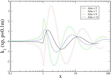
Figure 2: $P$-wave reduced $K$ matrix $k_{1}(xp,p)$ as function of $x$ for $p/m=0.1$ and various values of $\Lambda/m$, when $V_{S\,1}^{(0)}=0$. We have taken $\lambda=4.25$.

Since the choice of $\Lambda$ is arbitrary, the LO on-shell $k_{l}^{(0)}(p,p)$ should be independent of $\Lambda$ when $\Lambda$ is sufficiently large. But as shown $k_{l}(p,p)$ with $V_{S}^{(0)}=0$ oscillates with varying $\Lambda$ and the limit $\Lambda\to\infty$ is not well defined. Therefore this $k_{l}(p,p)$ and the associated observables are meaningless. RG invariance is not being respected in channels where the attractive singular potential is treated non-perturbatively and no counterterms are provided.

III.2 Renormalization of $-1/r^{2}$

The dependence on $\Lambda$ indicates that the $T$ matrix is sensitive to short-range physics through virtual states, that is, the loops resummed in the Lippmann-Schwinger equation, Fig. 1. However, the high-momentum part of the loops cannot be distinguished from contact interactions. The cutoff simply represents an arbitrary division of where short-range physics is placed. A model-independent accounting of this physics requires the introduction of contact interactions with parameters that depend on $\Lambda$ in such a way that observables are independent of $\Lambda$. Thus, with the technique of renormalization one can get a cutoff-independent amplitude. One has to renormalize each singular partial wave separately. We shall show here that one counterterm in each singular partial wave $l<l_{c}$ is necessary and sufficient to renormalize the corresponding partial-wave amplitude. This extends the results of Refs. beane ; coon ; hammer to waves beyond $S$.

For the $l$ wave, the contact interaction with fewest derivatives in coordinate space can be written in a partial-wave projection as

$$V_{S\,l}^{(0)}(p^{\prime},p)=\frac{\pi^{2}}{m}\frac{C_{l}^{(0)}(\Lambda)}{(2l+1)}{p^{\prime}}^{l}p^{l}\,,$$ (32)

where $C_{l}^{(0)}$ is a parameter. Equation (6) becomes

$$t_{l}^{(0)}(px,p) = -\frac{1}{2l+1}\left\{\lambda x^{-(l+1)}\,\left[\theta(x-1)-\int_{0}^{x}dy\,\frac{y^{l+2}}{y^{2}-1-i\epsilon}t_{l}^{(0)}(py,p)\right]\right.$$ (33)

$$\left.\qquad\qquad+\lambda x^{l}\,\left[\theta(1-x)-\int_{x}^{\Lambda/p}dy\,\frac{y^{1-l}}{y^{2}-1-i\epsilon}t_{l}^{(0)}(py,p)\right]\right.$$

$$\left.\qquad\qquad+C_{l}^{(0)}p^{2l+1}x^{l}\left[1-\int^{\Lambda/p}_{0}dy\,\frac{y^{l+2}}{y^{2}-1-i\epsilon}t_{l}^{(0)}(py,p)\right]\right\}\,,$$

instead of Eq. (18).

Renormalizing the $l$-wave amplitude means that the $\Lambda$ dependence of $C_{l}^{(0)}$ is such as to make the on-shell amplitude $t_{l}^{(0)}(p,p;\Lambda,C_{l}^{(0)}(\Lambda))$ independent of $\Lambda$ in the large-$\Lambda$ limit:

$$\Lambda\frac{d}{d\Lambda}t_{l}^{(0)}\left(p,p;\Lambda,C_{l}^{(0)}(\Lambda)\right)=O\left(\frac{p^{2}}{\Lambda^{2}}t_{l}^{(0)}\right)\;.$$ (34)

For $-1/r^{2}$, we will show that the half-off-shell $t_{l}^{(0)}(px,p;\Lambda,C_{l}(\Lambda))$ is also RG invariant in the large-$\Lambda$ limit,

$$\Lambda\frac{d}{d\Lambda}t_{l}^{(0)}\left(px,p;\Lambda,C_{l}^{(0)}(\Lambda)\right)=O\left(\frac{p^{2}}{\Lambda^{2}}t_{l}^{(0)}\right)\;.$$ (35)

To justify this claim we take it as an ansatz, evaluate the RG variation of the off-shell $t^{(0)}_{l}(px,p)$, and see if we can make it RG invariant by controlling $C_{l}^{(0)}$ with varying $\Lambda$. To this end, we take the total derivative with respect to $\Lambda$ of both sides of Eq. (33), assuming that $t^{(0)}(px,p;\Lambda,C_{l}^{(0)}(\Lambda))$ is RG invariant:

$$\frac{1}{2l+1}\left(\frac{xp}{\Lambda}\right)^{l}\left\{\left(\lambda-C_{l}^{(0)}\Lambda^{2l+1}\right)t_{l}^{(0)}(\Lambda,p)+(p\Lambda)^{l+1}\frac{dC_{l}^{(0)}}{d\Lambda}\left[1-I_{0,l}(p,\Lambda)\right]\right\}=O\left(\frac{p^{2}}{\Lambda^{2}}t_{l}^{(0)}\right)\;,$$ (36)

where we defined

$$I_{n,l}(p,\Lambda)=\int^{\Lambda/p}_{0}dy\,\frac{y^{2+2n+l}}{y^{2}-1-i\epsilon}\,t_{l}^{(0)}(py,p)\;.$$ (37)

Setting $x=\Lambda/p$ in Eq. (33),

$$t_{l}^{(0)}(\Lambda,p)=-\frac{1}{2l+1}\left(\lambda-C_{l}^{(0)}\Lambda^{2l+1}\right)\left(\frac{p}{\Lambda}\right)^{l+1}\left[1-I_{0,l}(p,\Lambda)\right]\;.$$ (38)

Eliminating the expression in the square brackets in Eqs. (36) and (38),

$$\left(\frac{xp}{\Lambda}\right)^{l}\frac{t_{l}^{(0)}(\Lambda,p)}{\lambda-C_{l}^{(0)}\Lambda^{2l+1}}\left[\frac{1}{2l+1}\left(\lambda-C_{l}^{(0)}\Lambda^{2l+1}\right)^{2}-\Lambda^{2(l+1)}\frac{dC_{l}^{(0)}}{d\Lambda}\right]=O\left(\frac{p^{2}}{\Lambda^{2}}t^{(0)}\right)\;.$$ (39)

Now, the left-hand side of Eq. (39) can be made of $O(p^{2}t^{(0)}/\Lambda^{2})$ for all $x$ by properly choosing $C_{l}^{(0)}(\Lambda)$, which is indeed consistent with the above ansatz that the half-off-shell $t_{l}^{(0)}(px,p)$ is RG invariant, up to $O(p^{2}/\Lambda^{2})$. This will be so if $C_{l}^{(0)}(\Lambda)$ satisfies the RG equation

$$\Lambda\frac{dC_{l}^{(0)}}{d\Lambda}\equiv\beta\left(C_{l}^{(0)}\right)=\frac{1}{(2l+1)\Lambda^{2l+1}}\left(\lambda-\Lambda^{2l+1}C_{l}^{(0)}\right)^{2}\,.$$ (40)

It is straightforward to solve for $C_{l}^{(0)}(\Lambda)$, up to a boundary condition:

$$C_{l}^{(0)}(\Lambda)=-\frac{\lambda}{\Lambda^{2l+1}}\frac{2l+1-2\nu_{l}\tan[\nu_{l}\ln(\Lambda/\Lambda_{*l})]}{2l+1+2\nu_{l}\tan[\nu_{l}\ln(\Lambda/\Lambda_{*l})]}\;,$$ (41)

where $\Lambda_{*l}$ is a dimensionful parameter defined in such a way that the reduced coupling $\Lambda_{*l}^{2l+1}C_{l}^{(0)}(\Lambda_{*l})=-\lambda$. It is determined by fitting to the measured $l$ partial-wave amplitude. The log-periodic behavior of $C_{l}^{(0)}$ is the so-called limit cycle 3bozos ; beane ; coon ; hammer ; limits .

Even with a non-zero $V_{S\,l}^{(0)}(p^{\prime},p)$ the integral equation (6) can be converted into Eq. (24). The same argument goes through with $\Lambda_{*l}$ substituted for $\Lambda$, dependence on which was eliminated, so that the RG-invariant half-off-shell $t^{(0)}_{l}(p^{\prime},p)$ in the $p^{\prime}\gg p$ limit is given by

$$t_{l}^{(0)}(px,p)=\mathcal{N}^{\prime}_{l}(p/\Lambda_{*l})\,x^{-\frac{1}{2}}\,\left[\cos\left(\nu_{l}\ln\frac{xp}{\Lambda_{*l}}\right)+\frac{1}{x^{2}}\cos\left(\nu_{l}\ln\frac{xp}{\Lambda_{*l}}+\beta_{l}\right)+O\left(\frac{1}{{x}^{4}}\right)\right]\,,$$ (42)

instead of Eq. (30). The phase is now fixed by $\Lambda_{*l}$, and observables are (nearly) cutoff independent.

To illustrate this we return to the $P$-wave example considered at the end of the previous subsection. To remove the cutoff dependence observed in Fig. 2, we solve for the $K$ matrix again but now with an additional short-range interaction $V_{S\,1}^{(0)}=\pi^{2}C_{1}^{(0)}p^{\prime}p/3m$ put in and allowed to change with $\Lambda$ in such a way that the on-shell $k_{1}^{(0)}(p,p)$ is independent of $\Lambda$. Figure 3 shows that not only the on-shell $k_{1}^{(0)}(p,p)$ but also the half-off-shell $k_{1}^{(0)}(p^{\prime},p)$ are now independent of $\Lambda$, in agreement with the previous argument. In this calculation we chose $\Lambda_{*1}/m=0.2$, but the results are qualitatively the same for any $\Lambda_{*1}$.

Figure 3: LO $P$-wave reduced $K$ matrix $k_{1}^{(0)}(xp,p)$ as function of $x$ for $p/m=0.1$, at various values of the cutoff $\Lambda$ in units of the reduced mass $m$, with $V_{S\,1}^{(0)}$ introduced to absorb the cutoff dependence. We have taken $\lambda=4.25$ and $\Lambda_{*1}/m=0.2$.

The net effect of renormalization is to replace $\Lambda$ by the physical quantities $\Lambda_{*l}$, which parametrize short-range interactions and are directly related to data. The appearance of dimensionful parameters (through renormalization with dimensionless parameters $\Lambda^{2l+1}C_{l}^{(0)}$ and $\lambda$) is an example of dimensional transmutation. These parameters introduce mass scales in the problem and break the scale invariance of the long-range potential —an example of an anomaly. (For an extensive discussion of this anomaly, see Ref. carlosanom .) Because of the log-periodic behavior, however, a discrete scale invariance remains, which has striking implications to observables hammer .

If only one channel ($l=0$) is singular, the trade off between $\Lambda$ and $\Lambda_{*0}$ is one-to-one; using $\Lambda_{*0}$ is formally equivalent to treating $\Lambda$ as a fit parameter. However, if more than one channel is singular at LO, more than one short-range parameter is present in the solution. Ignoring the counterterms and just fitting $\Lambda$ enforces a link between short-range parameters, which might or might not be correct. Regardless of whether this assumption is correct for a given problem, it is nothing but a model for the short-range physics, for it is a dynamical assumption that goes beyond the symmetry content of the theory. A model-independent treatment of short-range interactions requires at LO one counterterm per singular channel where perturbation theory does not apply.

IV $\pm 1/r^{4}$ as NLO long-distance interaction

We now turn to the effects of singular perturbations on the LO singular potential and its counterterms. We assume that the NLO long-range potential is given by Eq. (17), and ask which additional counterterms, if any, have to be supplied at NLO to make the result RG invariant. With our choice of parameters, the long-range potential, Eq. (17), is a correction to the LO long-range potential, Eq. (14), so the full NLO should have a small effect on observables. Accordingly, we treat the NLO potential $V^{(1)}$ in perturbation theory, that is, in first-order distorted-wave Born approximation. The NLO amplitude $T^{(1)}$ has one insertion of the NLO potential, see Fig. 4, that is,

$$t_{l}^{(1)}(p^{\prime},p) = \frac{mp}{\pi^{2}}V_{l}^{(1)}(p^{\prime},p)-2\int_{0}^{\Lambda}dq\frac{q}{q^{2}-p^{2}-i\epsilon}\frac{mq}{\pi^{2}}V_{l}^{(1)}(p^{\prime},q)t_{l}^{(0)}(q,p)$$ (43)

$$+\int_{0}^{\Lambda}dq^{\prime}\int_{0}^{\Lambda}dqt_{l}^{(0)}(p^{\prime},q^{\prime})\frac{q^{\prime}}{q^{\prime 2}-p^{2}-i\epsilon}\frac{mq^{\prime}}{\pi^{2}}V_{l}^{(1)}(q^{\prime},q)\frac{q}{{q}^{2}-p^{2}-i\epsilon}t_{l}^{(0)}(q,p)\;,$$

where we have used the symmetry of $V_{l}$ under exchange of its arguments. Two insertions of $V^{(1)}$ (second-order perturbation theory) come at next order, where further contributions to the long- and short-range potentials might exist.

Figure 4: NLO amplitude $T^{(1)}$ in first-order distorted-wave Born approximation in the NLO potential $V^{(1)}$.

For simplicity, we focus on the $S$ wave, $l=0$, in the following. Generalization to higher waves and higher orders is straightforward.

IV.1 Additional singularity

In principle new cutoff dependence, possibly divergent in the $\Lambda\to\infty$ limit, will arise from the loops in Fig. 4. Omitting for the moment any additional contact interactions in NLO, that is, taking $V_{S}^{(1)}=0$, let us consider the $\Lambda$ dependence of the on-shell amplitude. Taking the total derivative of Eq. (43) with respect to $\Lambda$ and using the fact that the off-shell $t_{0}^{(0)}(px,p)$ is RG invariant up to suppressed terms (see Eq. (35)), we find

$$\Lambda\frac{d}{d\Lambda}t_{0}(p,p) = -\frac{g\Lambda^{2}}{M^{2}}\left(1-\frac{p^{2}}{\Lambda^{2}}\right)^{-1}\left\{1-I_{0,0}(p,\Lambda)+\frac{p^{2}}{3\Lambda^{2}}\left[1-I_{1,0}(p,\Lambda)\right]\right\}t_{0}^{(0)}(\Lambda,p)$$ (44)

$$+O\left(\frac{p^{4}}{M^{2}\Lambda^{2}}t_{0}^{(0)}\right)\,,$$

where the integrals $I_{n,l}(p,\Lambda)$ were defined in Eq. (37). Using Eqs. (38) and (42) we can write

$$[1-I_{0,0}(p,\Lambda)]\,t_{0}^{(0)}(\Lambda,p)={\mathcal{N}}_{0}^{{}^{\prime}2}(p/\Lambda_{*0})\left[G_{0}\left(\frac{\Lambda}{\Lambda_{*0}}\right)+\frac{p^{2}}{\Lambda^{2}}G_{1}\left(\frac{\Lambda}{\Lambda_{*0}}\right)+O\left(\frac{p^{4}}{\Lambda^{4}}\right)\right]\;,$$ (45)

where $G_{0}$ and $G_{1}$ are two $p$-independent, oscillating functions of $\Lambda/\Lambda_{*0}$. A similar form can be obtained for the other term,

$$\frac{p^{2}}{\Lambda^{2}}[1-I_{1,0}(p,\Lambda)]t_{0}^{(0)}(\Lambda,p)={\mathcal{N}}_{0}^{{}^{\prime}2}(p/\Lambda_{*0})\left[H_{0}\left(\frac{\Lambda}{\Lambda_{*0}}\right)+\frac{p^{2}}{\Lambda^{2}}H_{1}\left(\frac{\Lambda}{\Lambda_{*0}}\right)+O\left(\frac{p^{4}}{\Lambda^{4}}\right)\right]\;,$$ (46)

in terms of two other oscillating functions $H_{0}$ and $H_{1}$ that do not depend on $p$. This can be seen from the cutoff dependence of $I_{1,0}(p,\Lambda)$ in the large-$\Lambda$ limit. We can write

$$I_{1,0}(p,\Lambda)=I_{0,0}(p,\Lambda)+\int_{\Lambda^{\prime}/p}^{\Lambda/p}dy\,y^{2}\,t_{0}^{(0)}(py,p)+\int_{0}^{\Lambda^{\prime}/p}dy\,y^{2}\,t_{0}^{(0)}(py,p)\;,$$ (47)

where $\Lambda^{\prime}$ is a scale above which the asymptotic expansion of $t_{0}^{(0)}$, Eq. (42), is valid. Since the $\Lambda$ dependence of the second integral is at most $\propto p^{2}/\Lambda^{2}$ (see Eq. (35)), $H_{0}$ and $H_{1}$ are given by the first integral.

Thus, Eq. (44) can be written as

$$\Lambda\frac{d}{d\Lambda}t_{0}(p,p) = -\frac{g}{M^{2}}{\mathcal{N}}_{0}^{{}^{\prime}2}(p/\Lambda_{*0})\left\{\Lambda^{2}\left[G_{0}\left(\frac{\Lambda}{\Lambda_{*0}}\right)+\frac{1}{3}H_{0}\left(\frac{\Lambda}{\Lambda_{*0}}\right)\right]\right.$$ (48)

$$+\left.p^{2}\left[G_{1}\left(\frac{\Lambda}{\Lambda_{*0}}\right)+G_{0}\left(\frac{\Lambda}{\Lambda_{*0}}\right)+\frac{1}{3}H_{1}\left(\frac{\Lambda}{\Lambda_{*0}}\right)+\frac{1}{3}H_{0}\left(\frac{\Lambda}{\Lambda_{*0}}\right)\right]+O\left(\frac{p^{4}}{\Lambda^{2}}\right)\right\}.$$

We find that there are two types of $\Lambda$-dependent terms (modulated by ${\mathcal{N}}_{0}^{{}^{\prime}2}$) that do not vanish in the large-$\Lambda$ limit: an energy-independent term whose oscillatory behavior gets enhanced by an arbitrary factor $\Lambda^{2}$, and a term that introduces further cutoff dependence proportional to the energy. This stronger cutoff dependence is just the momentum-space reflection of the higher singularity of $V_{L}^{(1)}$. Results become sensitive to the physics at the smaller distances where $V_{L}^{(1)}$ overcomes $V_{L}^{(0)}$. To account for this physics in a model-independent way, new counterterms are needed.

IV.2 NLO renormalization

Since $V_{L}^{(1)}$ is more singular than $V_{L}^{(0)}$ by two powers of momenta (c.f. Eqs. (14) and (17)), we expect, on the basis of dimensional analysis, that new counterterms with up to two extra derivatives or powers of $\Lambda$ will be required. Indeed, the two types of $\Lambda$ dependence in Eq. (48) suggest that we need two new counterterms, one being possibly just a correction to $C_{0}^{(0)}$. In that case, the running of $C_{0}$ is changed at NLO. For clarity, we split $C_{0}$ into two pieces, $C_{0}=C_{0}^{(0)}+C_{0}^{(1)}$, where $C_{0}^{(0)}(\Lambda)$ has the LO running given in Eq. (41) and $C_{0}^{(1)}(\Lambda)$ has an NLO running to be determined. However, this counterterm cannot be expected to eliminate the energy-dependent term. That requires a new counterterm $D_{0}^{(1)}$, which represents the leading energy dependence of the short-range physics, and whose running $D_{0}^{(1)}(\Lambda)$ should also be determined from the requirement of RG invariance of the $T$ matrix. These arguments suggest that the NLO short-range potential is

$$V_{S\,0}^{(1)}(p^{\prime},p)=\frac{\pi^{2}}{m}\left[C_{0}^{(1)}+D_{0}^{(1)}(p^{2}+{p^{\prime}}^{2})\right]\,.$$ (49)

Including these terms and using Eq. (38), we get, instead of Eqs. (44) and (48),

$$\Lambda\frac{d}{d\Lambda}t_{0}^{(1)}(p,p) = -\left\{\Lambda^{2}\left[1-I_{0,0}(p,\Lambda)\right]\left[\left(\frac{g}{M^{2}}+\frac{2C_{0}^{(1)}}{\Lambda}+2D_{0}^{(1)}\Lambda\right)\frac{\Lambda^{2}}{\Lambda^{2}-p^{2}}-\frac{1}{C_{0}^{(0)}\Lambda-\lambda}\frac{dC_{0}^{(1)}}{d\Lambda}\right]\right.$$ (50)

$$\left.+\;p^{2}\left[1-I_{1,0}(p,\Lambda)\right]\left[\left(\frac{g}{3M^{2}}+2D_{0}^{(1)}\Lambda\right)\frac{\Lambda^{2}}{\Lambda^{2}-p^{2}}-\frac{2\Lambda^{2}}{C_{0}^{(0)}\Lambda-\lambda}\frac{dD_{0}^{(1)}}{d\Lambda}\right]\right\}t_{0}^{(0)}(\Lambda,p)$$

$$+O\left(\frac{p^{4}}{M^{2}\Lambda^{2}}t_{0}^{(0)}\right)\,,$$

$$= -{\mathcal{N}}_{0}^{{}^{\prime}2}(p/\Lambda_{*0})\frac{\Lambda^{2}}{M^{2}}\left[R(\Lambda)+\frac{p^{2}}{\Lambda^{2}}S(\Lambda)+O\left(\frac{p^{4}}{\Lambda^{4}}\right)\right]\;,$$

where

$$\frac{1}{M^{2}}R(\Lambda) = G_{0}\left(\frac{\Lambda}{\Lambda_{*0}}\right)\left(\frac{g}{M^{2}}+\frac{2C_{0}^{(1)}}{\Lambda}+2D_{0}^{(1)}\Lambda-\frac{1}{C_{0}^{(0)}\Lambda-\lambda}\frac{dC_{0}^{(1)}}{d\Lambda}\right)$$ (51)

$$+\;H_{0}\left(\frac{\Lambda}{\Lambda_{*0}}\right)\left(\frac{g}{3M^{2}}+2D_{0}^{(1)}\Lambda-\frac{2\Lambda^{2}}{C_{0}^{(0)}\Lambda-\lambda}\frac{dD_{0}^{(1)}}{d\Lambda}\right)$$

and

$$\frac{1}{M^{2}}S(\Lambda) = G_{1}\left(\frac{\Lambda}{\Lambda_{*0}}\right)\left(\frac{g}{M^{2}}+\frac{2C_{0}^{(1)}}{\Lambda}+2D_{0}^{(1)}\Lambda-\frac{1}{C_{0}^{(0)}\Lambda-\lambda}\frac{dC_{0}^{(1)}}{d\Lambda}\right)$$ (52)

$$+\;H_{1}\left(\frac{\Lambda}{\Lambda_{*0}}\right)\left(\frac{g}{3M^{2}}+2D_{0}^{(1)}\Lambda-\frac{2\Lambda^{2}}{C_{0}^{(0)}\Lambda-\lambda}\frac{dD_{0}^{(1)}}{d\Lambda}\right)$$

$$+\;G_{0}\left(\frac{\Lambda}{\Lambda_{*0}}\right)\left(\frac{g}{M^{2}}+\frac{2C_{0}^{(1)}}{\Lambda}+2D_{0}^{(1)}\Lambda\right)+\;H_{0}\left(\frac{\Lambda}{\Lambda_{*0}}\right)\left(\frac{g}{3M^{2}}+2D_{0}^{(1)}\Lambda\right)\,.$$

It is clear that $C_{0}^{(1)}$ and $D_{0}^{(1)}$ generate terms with the same types of $\Lambda$ dependence as in Eq. (44). Therefore, by controlling $C_{0}^{(1)}$ and $D_{0}^{(1)}$, we can make both $R(\Lambda)=0$ and $S(\Lambda)=0$, and the NLO amplitude $t_{0}^{(1)}(p,p)$ becomes RG invariant up to $O(p^{4}/M^{2}\Lambda^{2})$.

Because the RG equations of the NLO counterterms $C_{0}^{(1)}(\Lambda)$ and $D_{0}^{(1)}(\Lambda)$ are not particularly illuminating, we turn to numerical experiments. We take $\lambda=2$, $g=1$ and $M=0.5m$. To test RG invariance, we define the fractional NLO correction

$$X(p,\Lambda)=\left|\frac{k_{0}^{(1)}(p,p;\Lambda)}{k_{0}^{(0)}(p,p;\Lambda)}\right|\,.$$ (53)

We first show that, in agreement with the previous argument, renormalization cannot be done with $C_{0}^{(1)}$ alone. We take as “datum” $k_{0}(0.1m,0.1m)=-1.05$. In LO, $C_{0}^{(0)}(\Lambda)$ is determined so as to reproduce this datum. The energy dependence is a prediction of the theory. In NLO, the additional terms in the potential will make the theory deviate from the datum, unless $C_{0}^{(1)}(\Lambda)$ is fitted to preserve agreement with the datum. We thus solve the Lippmann-Schwinger equation with various cutoffs, and find $C_{0}^{(1)}(\Lambda)$ such as to yield the datum. In Fig. 5 the dot-dashed line shows the fractional NLO correction $X(p,\Lambda)$ as function of $\Lambda$ for $p=0.175m$. It oscillates as $\Lambda$ increases and does not show sign of convergence. One concludes that $C_{0}^{(1)}$ by itself does not renormalize the NLO amplitude.

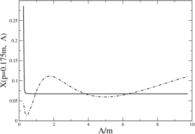
Figure 5: Fractional NLO correction $X(p,\Lambda)$ at $p=0.175m$ as function of $\Lambda/m$. The dot-dashed line is made by setting $D_{0}^{(1)}=0$ while the solid line employs both $C_{0}^{(1)}$ and $D_{0}^{(1)}$. We have taken $\lambda=2$, $g=1$, and $M/m=0.5$.

We now repeat the calculation but including both $C_{0}^{(1)}$ and $D_{0}^{(1)}$. Since two parameters are involved in the fit, $k_{0}(0.1m,0.1m)=-1.05$ and $k_{0}(0.15m,0.15m)=-0.34$ are used as “data”. The second data point is chosen as a 5% displacement of the value of $k_{0}^{(0)}(0.15m,0.15m)$, to ensure that at low momenta NLO represents a small effect on observables. The cutoff dependence of the fractional NLO correction at $p=0.175m$ is shown as the solid line in Fig. 5. The plateau in the solid line supports the hypothesis that the counterterms in Eq. (49) indeed renormalize the NLO amplitude.

With the data chosen above we compute the energy dependence of the amplitude. Figure 6 shows the energy dependence of both LO and LO+NLO reduced $K$ matrices. Both sets of results are computed with four different cutoffs $\Lambda/m=5.5,6.5,7.5$ and $8.5$: there are four data points on each spot in the figure. The fact that the points for different cutoffs are indistinguishable indicates that the amplitudes are being properly renormalized. It is seen that the NLO correction is small for $p\ll M$ and fails for $p\sim M$, as it should.

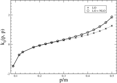
Figure 6: Reduced on-shell $K$ matrix $k_{0}(p,p)$ in the $S$ wave as a function of $p/m$, with $\Lambda/m=5.5,6.5,7.5$ and $8.5$: leading order (crosses) and up to next-to-leading order (circles). We have taken the same parameters as for the solid line in Fig. 5.

V Discussion

In the previous sections we tackled a number of issues in the rich physics of singular potentials using a simple toy model $-1/r^{2}\pm 1/r^{4}$. Most of our results are independent of this particular choice, but some are a consequence of the classical scale invariance of the LO potential. We discuss here some of the limitations and generalizations of these results to an LO potential of the form $-\lambda/2mM_{lo}^{n-2}r^{n}$, $n\geq 2$ and $\lambda=O(1)>0$, perturbed by a more singular potential. Here $M_{lo}$ is a characteristic scale that sets the curvature of the long-range potential. Clearly, at distances $r\sim 1/M_{lo}$ there can be a balance between kinetic repulsion and long-range attraction, so this is a natural size for a bound state or resonance to have. Accordingly, a momentum $Q\sim M_{lo}$ is the most interesting resolution to consider.

In Sect. III we presented a new method for the study of the Lippmann-Schwinger equation with a singular potential, in which we transformed it to a differential equation, Eq. (23). We would like to point out that this method can be applied to all $1/r^{2m}$ ($m$ an integer) potentials, in which case we obtain a generalization of Eq. (23) that involves the $m$th-order Laplacian . The corresponding solutions then have similar properties. An extension of the calculations of this paper to the more general case is under investigation lbw .

We have shown that angular momentum plays an important, double role through the repulsive effects of the centrifugal barrier. The emergence of the remarkable phenomena we discussed comes from the competition between the singular potential and the centrifugal barrier. When $n=2$, for a given singular potential strength, there is a critical angular momentum $l_{c}$, Eq. (31), above which the effective radial potential is no longer attractive, and the particles are prevented from probing short-range physics. In these waves, the problem is well defined in LO without a short-range counterterm. Conversely, in waves with $l<l_{c}$, a counterterm is required in every wave, in agreement with a general argument behncke68 . Such a critical angular momentum is a particularity of $n=2$. For $n>2$, the singular potential will overcome the centrifugal barrier (with $l>0$) at some distance $r_{l}\sim(\lambda/l(l+1))^{1/(n-2)}/M_{lo}$. Therefore, the two particles will want to get as close as allowed by short-range physics. To make observables minimally sensitive to this short-range physics, a single counterterm is required in every wave. Only recently was this found nogga_timmermans_vankolck ; spaniards1 in the more complicated case of the direction-dependent $1/r^{3}$ potential originating from one-pion exchange between nucleons.

Regardless of the existence of $l_{c}$, the centrifugal barrier weakens (for $n=2$) or dominates (for $n>2$) over the singular potential at large distances. The larger the $l$, the weaker the effective radial potential in a partial wave. This leads for $n=2$ to a second value for $l$, $l_{p}$ in Eq. (21), above which the potential can be treated in perturbation theory. When $n>2$, there is always a spatial region $r<r_{l}$ where the singular potential is strong, but its size decreases with $l$. Whether the potential can be treated in perturbation theory in a given partial wave depends then crucially on the range of momenta $Q$ that we are interested in probing. For a given $Q$, a sufficiently large $l$ exists where the support of the strong potential is effectively a short-range effect. For short-range potentials, barring fine-tunings leading to bound states or resonances at threshold, perturbation theory holds in higher waves goldberger . In the nuclear case below the QCD mass scale, it was found that $l_{p}\approx 3$ nogga_timmermans_vankolck .

It is thus a general feature of singular potentials that a single counterterm, Eq. (32), is needed in all waves where the potential is sufficiently attractive. For $n=2$, the presence of dimensionful parameters $\Lambda_{*l}$ breaks scale invariance, but discrete scale invariance remains in the form of limit cycle. Our LO results in the $S$ wave are essentially the same as in the three-body system with short-range interactions 3bozos ; coverass2 . For $n>2$, the dependence of counterterms on the cutoff is slightly more complicated, but still oscillatory beane ; mary .

The renormalization of $-1/r^{n}$ suggests a different power counting than what one would expect from naive dimensional analysis (NDA) or naturalness. Based on NDA one would expect that $C_{l}$ in Eq. (32) scales as

$$C_{l}\sim\frac{1}{M_{hi}^{2l+1}}\,.$$ (54)

This is reasonable if $\lambda$ is outside of the singular region or if the Born approximation is valid. But if this is not the case the necessity of renormalization promotes $C_{l}$ to the same size as the long-range potential. The renormalized $C_{l}$ can be thought of as scaling instead with the resolution $Q$ at which the potential is considered valid,

$$C_{l}^{(0)}\sim\frac{\lambda}{Q^{2l+1}}\,.$$ (55)

The corresponding short-range interaction, Eq. (32), then scales as $1/mQ$, which is the same scaling as the long-range potential.

In Sect. IV we investigated the effects of a perturbation in the form of a singular potential with two more powers of momenta than the LO potential: a $(Q/M_{hi})^{2}$ perturbation. In the nuclear case, it has been suggested nogga_timmermans_vankolck and disputed spaniards2 that the additional counterterms are those indicated by NDA, in this case, those with two more powers of momenta. We found here that a perturbative treatment of the corrections is indeed consistent with this NDA expectation.

Therefore, once the failure of NDA is corrected at LO, Eq. (55), power counting is formulated as usual. In the particular example considered here, Eq. (49),

$$C_{0}^{(1)}\sim\frac{gQ}{M_{hi}^{2}}\,,\qquad D_{0}^{(1)}\sim\frac{g}{QM_{hi}^{2}}\,.$$ (56)

As a consequence, the NLO short-range interaction, Eq. (49), scales as $gQ/mM_{hi}^{2}$, just as the NLO long-range potential.

We can also use the arguments of Sect. IV to determine the NLO counterterms if the NLO long-distance potential is another potential than $1/r^{4}$. For example, in the case of $1/mM_{hi}^{4}r^{6}$ as NLO, whose Fourier transform is $\sim Q^{3}/mM_{hi}^{4}$, one expects to need

$$C_{0}^{(1)}+D_{0}^{(1)}({p^{\prime}}^{2}+p^{2})+E_{0}^{(1)}{p^{\prime}}^{2}p^{2}$$ (57)

as NLO counterterms in the $S$ wave, based on the qualitative arguments of Sect. IV. In this case

$$C_{0}^{(1)}\sim\frac{gQ^{3}}{M_{hi}^{4}}\,,\qquad D_{0}^{(1)}\sim\frac{gQ}{M_{hi}^{4}}\,,\qquad E_{0}^{(1)}\sim\frac{g}{QM_{hi}^{4}}\,,$$ (58)

so that the short-range interaction scales as $gQ^{3}/mM_{hi}^{4}$.

This state of affairs is perhaps not surprising. NDA was developed based on experience with perturbation theory. It does fail for an attractive singular potential, but only when the potential is treated non-perturbatively in LO. Once this unforeseen event is incorporated in the power counting, the perturbative treatment of the corrections conforms to NDA, relative to the corrected LO.

VI Summary and Outlook

We have used $-1/r^{2}\textrm{(LO)}\pm 1/r^{4}\textrm{(NLO)}$ as an example to demonstrate how to build effective theories based upon singular potentials. The key point is to understand the power counting of contact interactions. The correct power counting scheme should consist of the minimum set of contact interactions that renormalizes scattering amplitudes including the long-range potentials. Due to this intrinsic relation between renormalization and power counting it was found that the sizes of contact interactions are different from what is expected by naive dimensional analysis.

A new approach to the renormalization of a $-1/r^{2}$ potential was presented. It was shown that the singularity of $-1/r^{2}$ depends on angular momentum. The region of singularity entangles with that of validity of the Born approximation. In each partial wave where the LO potential is resummed to all orders, a single counterterm is needed for renormalization. The NLO potential can be treated as a (distorted-wave) perturbation, and the minimum set of NLO short-range counterterms that are needed to renormalize the NLO amplitude can be determined by estimating the superficial cutoff dependence with the asymptotic LO $T$ matrix. Analytical arguments were supplemented by numerical evidence.

It is one of the main conclusions of this paper that the power counting, a key ingredient of any effective theory, cannot be decided solely on the basis of naive dimensional analysis in the case of (non-perturbative) singular potentials. One has to rely on explicit checks of RG invariance, either analytical or numerical, in order to test any proposed power counting scheme. Yet, once LO has been understood, perturbative corrections do not violate naive dimensional analysis with respect to LO.

Besides nuclear forces weinberg ; others ; towards ; nogga_timmermans_vankolck ; spaniards1 ; germans ; spaniards2 ; sameold , there may be other applications of effective theories of singular potentials. For example, the $1/r^{2}$ potential in two dimensions is relevant for the interaction of a neutral atom with a charged wire (see, e.g., Ref. denschlag ), while it appears in three dimensions with an angle-dependent coefficient when a charge is in the field of a polar molecule (see, e.g. Ref. leblond ). Our results could be readily applied to long-range corrections in these systems . With extensions lbw , it could also be applied to the (long-range) electron-atom interaction, which is often divided into $-1/r^{4}$, $1/r^{6}$ and higher terms frank_land_spector . In all these cases, one can construct effective theories with a well defined power counting that incorporate renormalization-group ideas.

- (1) W.M. Frank, D.J. Land, and R.M. Spector, Rev. Mod. Phys. 43 (1971) 36.
- (2) K.M. Case, Phys. Rev. 80 (1950) 797.
- (3) S.R. Beane, P.F. Bedaque, L. Childress, A. Kryjevski, J. McGuire, and U. van Kolck, Phys. Rev. A 64 (2001) 042103.
- (4) M. Bawin and S.A. Coon, Phys. Rev. A 67 (2003) 042712; E. Braaten and D. Phillips, hep-th/0403168; H.E. Camblong and C.R. Ordóñez, Phys. Lett. A 345 (2005) 22.
- (5) H.-W. Hammer and B.G. Swingle, Ann. Phys. 321 (2006) 306.
- (6) M. Alberg, M. Bawin, and F. Brau, Phys. Rev. A 71 (2005) 022108.
- (7) P.F. Bedaque, H.-W. Hammer, and U. van Kolck, Phys. Rev. Lett. 82 (1999) 463; Nucl. Phys. A 646 (1999) 444; Nucl. Phys. A 676 (2000) 357.
- (8) S.D. Głazek and K.G. Wilson, Phys. Rev. Lett. 89 (2002) 230401; 92 (2004) 139901 (E); Phys. Rev. B 69 (2004) 094304; S.D. Głazek, Phys. Rev. D 75 (2007) 025005; E.J. Mueller and T.-L. Ho, cond-mat/0403283; A. Morozov and A.J. Niemi, Nucl. Phys. B 666 (2003) 311; A. Morozov, hep-th/0502010; D. Bernard and A. LeClair, Phys. Lett. B 512 (2001) 78; A. LeClair, J.M. Roman, and G. Sierra, Nucl. Phys. B 675 (2003) 584; Phys. Rev. B 69 (2004) 020505(R); Nucl. Phys. B 700 (2004) 407; A. LeClair and G. Sierra, J. Stat. Mech. 0408 (2004) P004; A. Anfossi, A. LeClair, and G. Sierra, J. Stat. Mech. 0505 (2005) P011; G. Sierra, J. Stat. Mech. 0512 (2005) P006; Y. Meurice and M.B. Oktay, Phys. Rev. D 69 (2004) 125016.
- (9) H. Behncke, Nuovo Cimento 55A (1968) 780.
- (10) S.R. Beane, P.F. Bedaque, M.J. Savage, and U. van Kolck, Nucl. Phys. A 700 (2002) 377.
- (11) A. Nogga, R.G.E. Timmermans and U. van Kolck Phys. Rev. C 72 (2005) 054006; M.C. Birse, Phys. Rev. C 74 (2006) 014003; arXiv:0706.0984 [nucl-th].
- (12) M. Pavón Valderrama and E. Ruiz Arriola, Phys. Rev. C 74 (2006) 064004.
- (13) E. Epelbaum and U.-G. Meißner, nucl-th/0609037.
- (14) S. Weinberg Phys. Lett. B 251 (1990) 288; Nucl. Phys. B 363 (1991) 3; C. Ordóñez and U. van Kolck, Phys. Lett. B 291 (1992) 459; C. Ordóñez, L. Ray, and U. van Kolck, Phys. Rev. Lett. 72 (1994) 1982; Phys. Rev. C 53 (1996) 2086.
- (15) N. Kaiser, R. Brockmann, and W. Weise, Nucl. Phys. A 625 (1997) 758; J.L. Friar, Phys. Rev. C 60 (1999) 034002.
- (16) U. van Kolck, Prog. Part. Nucl. Phys. 43 (1999) 337; E. Epelbaum, Prog. Part. Nucl. Phys. 57 (2006) 654.
- (17) M. Pavón Valderrama and E. Ruiz Arriola, Phys. Rev. C 74 (2006) 054001.
- (18) T. Frederico, V.S. Timóteo, and L. Tomio, Nucl. Phys. A 653 (1999) 209; V.S. Timóteo, T. Frederico, A. Delfino, and L. Tomio, Phys. Lett. B 621 (2005) 109; M.C. Birse, J.A. McGovern, and K.G. Richardson, Phys. Lett. B 464 (1999) 169; T. Barford and M.C. Birse, Phys. Rev. C 67 (2003) 064006; C.-J. Yang, Ch. Elster, and D.R. Phillips, arXiv:0706.1242v1 [nucl-th].
- (19) H.-W. Hammer and T. Mehen, Nucl. Phys. A 690 (2001) 535; I.R. Afnan and D.R. Phillips, Phys. Rev. C 69 (2004) 034010.
- (20) P.F. Bedaque, G. Rupak, H.W. Grießhammer, and H.-W. Hammer, Nucl. Phys. A 714 (2003) 589; H.W. Grießhammer, Nucl. Phys. A 760 (2005) 110; Few-Body Syst. 38 (2006) 67; L. Platter and D.R. Phillips, Few-Body Syst. 40 (2006) 35; L. Platter, Phys. Rev. C 74 (2006) 037001.
- (21) T. Barford and M.C. Birse, J. Phys. A 38 (2005) 697.
- (22) H.E. Camblong and C.R. Ordóñez, Phys. Rev. D 68 (2003) 125013; H.E. Camblong, L.N. Epele, H. Fanchiotti, C.A. García Canal, and C.R. Ordóñez, Phys. Lett. A 364 (2007) 458.
- (23) B. Long, in progress.
- (24) M.L. Goldberger and K.M Watson, Collision Theory (Krieger Publishing, New York, 1975).
- (25) J. Denschlag and J. Schmiedmayer, Europhys. Lett. 38 (1997) 405; J. Denschlag, G. Umshaus, and J. Schmiedmayer, Phys. Rev. Lett. 81 (1998) 737; M. Bawin and S.A. Coon, Phys. Rev. A 63 (2001) 034701; G.N.J. Añaños, H.E. Camblong, C.R. Ordóñez, Phys. Rev. D 68 (2003) 025006.
- (26) J.-M. Lévy-Leblond, Phys. Rev. 153 (1967) 1; J.-M. Lévy-Leblond and J.P. Provost, Phys. Lett. B 26 (1967) 104; O.H. Crawford, Proc. Phys. Soc. 91 (1967) 279; C. Desfrançois, H. Abdoul-Carime, N. Khelifa, and J. P. Schermann, Phys. Rev. Lett. 73 (1994) 2436; H.E. Camblong, L.N. Epele, H. Fanchiotti, and C.A. García Canal, Phys. Rev. Lett. 87 (2001) 220402; H.E. Camblong, L.N. Epele, H. Fanchiotti, C.A. García Canal, and C.R. Ordóñez, Phys. Rev. A 72 (2005) 032107.
- (27) V.N. Efimov, Sov. J. Nucl. Phys. 12 (1971) 589; P.F. Bedaque, in Nuclear Physics with Effective Field Theories, R. Seki, U. van Kolck, and M.J. Savage (editors), World Scientific, Singapore (1998), nucl-th/9806041.