Beyond the standard entropic inequalities: stronger scalar separability criteria and their applications.

Abstract

Recently it was shown that if a given state fulfils the reduction criterion, it must also satisfy the known entropic inequalities. The natural question arises as to whether it is possible to derive some scalar inequalities stronger than the entropic ones, assuming that stronger criteria based on positive but not completely positive maps are satisfied. In the present paper we show that if certain conditions hold, the extended reduction criterion [H.-P. Breuer, Phys. Rev. Lett 97, 080501 (2006); W. Hall, J. Phys. A 40, 6183 (2007)] leads to some entropic-like inequalities, much stronger than their entropic counterparts. The comparison of the derived inequalities with other separability criteria shows that such an approach might lead to strong scalar criteria detecting both distillable and bound entanglement. In particular, in the case of $\mathrm{SO}(3)$-invariant states it is shown that the present inequalities detect entanglement in regions, in which linear entanglement witnesses based on the extended reduction map fail. It should also be emphasized that in the case of $2\otimes d$ states the derived inequalities detect entanglement efficiently, while the extended reduction maps are useless, when acting on the qubit subsystem. Moreover, there is a natural way to construct a many-copy entanglement witnesses based on the derived inequalities so, in principle, there is a possibility of experimental realization. Some open problems and possibilities for further research are outlined.

1 Introduction.

Quantum entanglement, well understood for pure states EPR ; Sch , was much later formalized for mixed states Werner and developed into a key ingredient of quantum information theory, including especially quantum communication (see Ref. RevModPhys , and references therein). In the bipartite case, a mixed quantum state acting on a finite-dimensional Hilbert space ${\cal H}_{AB}=\mathcal{H}_{A}\otimes\mathcal{H}_{B}$ is called separable if and only if it is of the form Werner

$$\varrho=\sum_{i}p_{i}\rho^{(i)}_{A}\otimes\tilde{\rho}^{(i)}_{B}.$$ (1.1)

Otherwise it is called entangled or inseparable. In the above formula $\rho_{A}^{(i)}$ and $\tilde{\rho}_{B}^{(i)}$ are density matrices acting on the Hilbert spaces $\mathcal{H}_{A}$ and $\mathcal{H}_{B}$, respectively, $p_{i}\geq 0$ and $\sum_{i}p_{i}=1$. The definition is consistent with the pure state scenario, in which the state is entangled if and only if the vector representing it $|\psi\rangle\in\mathcal{H}_{A}\otimes\mathcal{H}_{B}$ is not a tensor product of vectors describing the subsystems

$$|\psi\rangle\neq|\varphi\rangle\otimes|\phi\rangle,$$ (1.2)

where $|\varphi\rangle\in\mathcal{H}_{A}$ and $|\phi\rangle\in\mathcal{H}_{B}$.

Schrödinger Sch pointed out that the essence of pure entangled state is of the informational kind, i.e., the total information about the system exceeds the information about its subsystems. In fact, the total information is maximal (since the state is pure) while the local ones are not (since the subsystems are mixed). For mixed states the above Schrödinger intuition was first formalized in terms of the von Neumann entropy $S_{1}(\varrho)=-\mathrm{Tr}(\varrho\log\varrho)$. Namely, it was observed in Ref. RPHPLA that any separable state has to obey the converse rule, i.e., it must have the entropy of the total system greater than entropies of the subsystems

$$S_{1}(\varrho_{A})\leq S_{1}(\varrho)\quad\mathrm{and}\quad S_{1}(\varrho_{B})\leq S_{1}(\varrho),$$ (1.3)

where $\varrho_{A(B)}=\mathrm{Tr}_{B(A)}\varrho$. Thus any violation of the above conditions implies entanglement (see also Ref. Plastino for an analysis of special examples). Recently this fact was shown to play a central role in the quantum version of Slepian-Wolf theorem Nature , which solves the long-standing open problem (analyzed first for pure states in Ref. CA ) of full physical interpretation of negative quantum conditional entropy $S_{1}(\varrho)-S_{1}(\varrho_{A})$. In particular, it stimulated the development of operational approach to other quantum conditional quantities DevetakYard . Note also that the conditional entropy of another kind, based on $\alpha$-entropy with $\alpha=\infty$ (see below), happens to play an important role in some cryptographic scenarios Renner .

The condition (1.3) belongs to the so-called scalar criteria of entanglement. Its generalization, stating that any separable state should satisfy

$$S_{\alpha}(\varrho_{A})\leq S_{\alpha}(\varrho)\quad\mathrm{and}\quad S_{\alpha}(\varrho_{B})\leq S_{\alpha}(\varrho)\quad(\alpha\in[0,\infty))$$ (1.4)

were derived first for special values of the parameter $\alpha$ RPHPLA ; HHHEntr ; CAG and special class of separable states MRHPRA . Later Eq. (1.4) was proved to hold for the whole range of $\alpha\in[0,\infty)$ Terhal3 ; VollbrechtWolf . Here, by $S_{\alpha}$ we denote, e.g., the Renyi entropy defined as

$$S_{\alpha}^{R}=\frac{1}{1-\alpha}\log\mathrm{Tr}\varrho^{\alpha}.$$ (1.5)

Straightforward calculations lead to more operational forms of the inequalities (1.4), which for $\alpha\in(1,\infty)$ become

$$\mathrm{Tr}\varrho_{A}^{\alpha}\geq\mathrm{Tr}\varrho^{\alpha}\quad\mathrm{and}\quad\mathrm{Tr}\varrho_{B}^{\alpha}\geq\mathrm{Tr}\varrho^{\alpha},$$ (1.6)

while for $\alpha\in[0,1)$,

$$\mathrm{Tr}\varrho_{A}^{\alpha}\leq\mathrm{Tr}\varrho^{\alpha}\quad\mathrm{and}\quad\mathrm{Tr}\varrho_{B}^{\alpha}\leq\mathrm{Tr}\varrho^{\alpha}.$$ (1.7)

Let us recall that for $\alpha=1$ the Renyi entropy reduces to the von Neumann entropy $S_{1}$. For $\alpha=0$ we have $S_{0}^{R}(\varrho)=R(\rho)$ with $R(\cdot)$ denoting the rank of a given matrix. Finally, for $\alpha=\infty$, $S^{R}_{\infty}(\varrho)=-\log||\varrho||$, where $||\cdot||$ is a standard operator norm. Thus for $\alpha=\infty$ the conditions (1.4) become MHPH :

$$||\varrho_{A}||\geq||\varrho||\quad\mathrm{and}\quad||\varrho_{B}||\geq||\varrho||.$$ (1.8)

It is worth mentioning that the above entropic criteria can be viewed as a prototype of nonlinear separability criteria that has been recently intensively developed in Refs. nonlinear ; Guhne . In particular, the new class of entropic inequalities that involve Klein-like entropies, i.e., entropies of output statistics of measurements Guhne .

Recently an experimental illustration of the inequality (1.6) for $\alpha=2$ has been performed Bovino . For experimental realizations of other quantitative and qualitative nonlinear separability tests see, e.g., Ref. spinsqetal .

Apart form the scalar criteria discussed above, the so called structural criteria were introduced Peres ; HHHPLA96 and investigated (see Ref. maps and references therein). Here we shall especially need the separability conditions based on positive but not completely positive maps HHHPLA96 (denoted hereafter by $\Lambda$) with the positive partial transposition (PPT) criterion Peres as the most famous example. Positive maps, characterizing separability themselves, allow also for introduction of a dual picture, i.e., the description in terms of the so-called entanglement witnesses HHHPLA96 ; Terhal1 ; Terhal2 . Let us recall, that a Hermitian operator $W$ is called an entanglement witness if its mean value on all separable states is nonnegative and negative for at least one entangled state. Entanglement witnesses lead to a popular method of experimental entanglement detection nowadays (see Ref. RevModPhys ). However, some other indirect applications of the positive map criterion were also proposed. In particular, the possible measurement of certain functionals of $\varrho$ and $[I\otimes\Lambda](\varrho)$ was discussed in Refs. Carteret ; PHRAMD . Here and further by $I$ we shall be denoting an identity map.

One of the criteria, based on positive maps and important from the communication point of view is the so-called reduction criterion reduction2 ; xor . It arises from the reduction map, which acts on a $d\times d$ matrix $A$ as $\Lambda_{r}(A)=(\mathrm{Tr}A)\mathbbm{1}_{d}-A$. The criterion states that any separable state $\varrho$ acting on $\mathbb{C}^{d_{A}}\otimes\mathbb{C}^{d_{B}}$, should retain a nonnegative spectrum after the action of the map $I\otimes\Lambda_{r}$, leading to the following operator inequality:

$$\varrho_{A}\otimes\mathbbm{1}_{d_{B}}\geq\varrho.$$ (1.9)

In Ref. CAG the above criterion was shown to imply the first entropic inequality (1.3). Later in Ref. VollbrechtWolf the implication was extended to all entropic inequalities. In this way the criterion based on the positive map provided the series of scalar criteria which for a natural number $\alpha$ may be measured via the collective entanglement witnesses (see, e.g., Refs. Bovino ; PH3 ).

In analogy to Refs. CAG ; VollbrechtWolf it is natural to ask a general question. Is it possible to derive entropic-like inequalities from other positive maps than the reduction one?

Recently, a new positive map, whose structure is similar to the reduction map, has been introduced in Refs. Bcrit ; Bcrit2 ; Hall . The map leads to the following operator inequality

$$\varrho_{A}\otimes\mathbbm{1}_{d_{B}}\geq\varrho+\varrho^{\tau_{B}^{U}},$$ (1.10)

and unlike the reduction map, was shown to be indecomposable. As such it can detect PPT entangled states BE . Here $\tau_{B}^{U}$ stands for partial transposition with respect to subsystem $B$ composed with a local antisymmetric operation $U$ such that $U^{\dagger}U\leq\mathbbm{1}_{d}$ on the second subsystem. Of course, one may write a similar operator inequality for the subsystem $A$. Using this map we give a partially positive answer to the posed question. For a large class of states satisfying additional assumptions (including, in particular, the states that are isomorphic to quantum channels) we derive a series of entropic-like inequalities which detect entanglement better than their entropic counterparts. We derive also the operator version of the inequalities.

The paper is organized as follows. The detailed construction of the inequalities is given in Sec. 2. At the beginning we discuss the case of two-particle states consisting of a qubit and qudit (qubit-qudit states) to introduce the method and discuss some special cases and examples. Then we present the inequalities for higher-dimensional systems and give some illustrative examples. In particular, we compare the derived inequalities with the entropic inequalities and entanglement witness arising from the Breuer criterion Bcrit . In Sec. 3 we present the corresponding multicopy entanglement witness. In Sec. 4 we discuss in more details a special inequality which, similarly to the entropic one for $\alpha=2$, can be measured as a collective entanglement witness on two copies of a state. Finally, using the fact that bipartite systems of even dimensions can be simulated by multiqubit states we show in Secs. 4.2 and 4.3 how to check the inequality experimentally within coalescence-anticoalescence experimental setups known already from the literature Bovino .

2 Inequalities

The construction of entropic-like inequalities is based on the recently introduced positive but not completely positive indecomposable map Bcrit , which acts on a $d\times d$ matrix $A$ (here $d$ is an even number) as follows:

$$\Lambda_{B}(A)=(\mathrm{Tr}A)\mathbbm{1}_{d}-A-A^{\tau}.$$ (2.1)

The symbol ${\tau}$ denotes the time reversal of $A$, namely $A^{\tau}=VA^{T}V^{\dagger}$, where $V$ is an antisymmetric anti-diagonal unitary matrix with anti-diagonal elements $\pm 1$, $\mathbbm{1}_{d}$ is a $d\times d$ identity matrix, and superscript $T$ denotes the matrix transposition in the standard basis. This map belongs to the class of indecomposable positive maps $\Lambda_{U}^{(-)}$ introduced by Hall Hall , where instead of the particular $V$, an arbitrary antisymmetric $(U^{T}=-U)$ matrix $U$ such that $U^{\dagger}U\leq\mathbbm{1}_{d}$ is taken. The map can be written in the following form

$$\Lambda_{U}^{(-)}(A)=(\mathrm{Tr}A)\mathbbm{1}_{d}-A-UA^{T}U^{\dagger}.$$ (2.2)

Note that for even $d$ one may take $U$ to be unitary since only in this case antisymmetric unitaries exist Hall . In further considerations we will concentrate on the special case considered by Breuer Bcrit , however, throughout the paper we will state the facts for general map $\Lambda_{U}^{(-)}$ whenever possible.

Let us also introduce a positive map similar to the Breuer-Hall map that will become useful in further considerations. The only difference a is a change of the sign before the modified transposition map, i.e.,

$$\Lambda_{U}^{(+)}(A)=(\mathrm{Tr}A)\mathbbm{1}_{d}-A+UA^{T}U^{\dagger},$$ (2.3)

where A is again a $d\times d$ matrix. The proof of positivity goes along the same lines as the proof for Breuer-Hall criterion given in Refs. Bcrit ; Hall . Notice that $\Lambda_{r}=(1/2)[\Lambda_{U}^{(+)}+\Lambda_{U}^{(-)}]$ and $\tau^{U}=(1/2)[\Lambda_{U}^{(+)}-\Lambda_{U}^{(-)}]$.

Before we state the main results let us introduce the following notations:

$$X^{\tau^{U}}=UX^{T}U^{\dagger}=\tau^{U}(X),$$ (2.4)

$\tau_{A}^{U}=\tau^{U}\otimes I$, and, respectively, $\tau_{B}^{U}=I\otimes\tau^{U}$. As previously stated, in particular case when $U=V$, the notation $\tau^{V}\equiv\tau$ shall be used. Finally, we shall denote the standard partial transposition with respect to the subsystem $A(B)$ by superscript $T_{A(B)}$, i.e., $[I\otimes T](X)=X^{T_{B}}$ and $[T\otimes I](X)=X^{T_{A}}$.

2.1 The case of qubit-qudit

As an introductory example we present the entropic-type inequalities for the qubit-qudit states. It should be emphasized that the Breuer map $\Lambda_{B}$ cannot be used as a separability criterion in the case of the qubit-qudit states (when the map acts on the smaller subsystem), since it gives zero on arbitrary projector acting on $\mathbbm{C}^{2}$. (Hall map $\Lambda_{U}^{(-)}$ is equivalent to Breuer map in this case, since each unitary antisymmetric matrix $U$ acting on the two dimensional subsystem can be written as $e^{i\phi}V$, which does not change the map). However, it does not mean that it is not useful in detecting entanglement at all. As we will see below it is a good starting point for derivation of some inequalities.

Let us first recall the Hilbert-Schmidt form of any qubit-qudit state. If we denote by $\varrho$ the density operator acting on the Hilbert space $\mathbb{C}^{2}\otimes\mathbb{C}^{d}$ and $\{f_{i}\}$ the generators of $\mathrm{SU}(d)$ with $f_{0}=\mathbbm{1}_{d}$, then the density matrix $\varrho$ might be written in the product basis $\{\sigma_{i}\otimes f_{j}\}$ as

$$\varrho=\frac{1}{2d}\sum_{i=0}^{3}\sum_{j=0}^{d^{2}-1}\xi_{ij}\sigma_{i}\otimes f_{j}.$$ (2.5)

On the first subsystem the basis is chosen to be Pauli matrices defined as

$$\sigma_{1}=\left(\begin{array}[]{cc}0&1\\ 1&0\end{array}\right),\quad\sigma_{2}=\left(\begin{array}[]{cc}0&-i\\ i&0\end{array}\right),\quad\sigma_{3}=\left(\begin{array}[]{cc}1&0\\ 0&-1\end{array}\right)$$ (2.6)

with $\sigma_{0}=\mathbbm{1}_{2}$. Coefficients $\xi_{ij}$ are given by $\xi_{ij}=(d/2)\mathrm{Tr}(\varrho\sigma_{i}\otimes f_{j})$, $\xi_{00}=1$, $\xi_{i0}=\mathrm{Tr}\varrho_{A}\sigma_{i}$, $\xi_{0j}=\mathrm{Tr}\varrho_{B}\sigma_{j}$, and thus real. The convention is such that $\mathrm{Tr}f_{i}f_{j}=2\delta_{ij}$, for $i=1,\ldots,d$.

In the Hilbert-Schmidt formalism one may easily recognize how the map $\tau_{A}$ acts on $\varrho$. When acting on the two-dimensional subsystem the unitary matrix $V$ is just $-i\sigma_{2}$. Thus, for arbitrary $j=0,1,2,3$ we have the following relation:

$$V\sigma_{j}V^{\dagger}=\sigma_{2}\sigma_{j}\sigma_{2}=2\delta_{2j}\sigma_{j}-\sigma_{j}=(-1)^{j}\sigma_{j},$$ (2.7)

which, in turn, implies that $\varrho^{\tau_{A}}$ has the following Hilbert-Schmidt representation:

$$\varrho^{\tau_{A}}=\frac{1}{2d}\left(\sum_{j=0}^{d^{2}-1}\xi_{0j}\mathbbm{1}_{2}\otimes f_{j}-\sum_{i=1}^{3}\sum_{j=0}^{d^{2}-1}\xi_{ij}\sigma_{i}\otimes f_{j}\right).$$ (2.8)

Comparison of Eqs. (2.5) and (2.8) leads immediately to the fact that $\varrho+\varrho^{\tau_{A}}=\mathbbm{1}_{2}\otimes\varrho_{B}$. Thus the Beuer map (2.1) indeed gives zero when acting on the two-dimensional subsystem. On the other hand, one recognizes in this equality the equivalence between transposition and reduction maps when both act on a $2\times 2$ matrix xor ; reduction2 , i.e., $\Lambda_{r}(A)=\tau(A)$. Following Ref. VollbrechtWolf and using the above relations we may write the following equalities for $\alpha\geq 1$:

$$\mathrm{Tr}\varrho_{B}^{\alpha} = \mathrm{Tr}\varrho(\mathbbm{1}_{2}\otimes\varrho_{B}^{\alpha-1})=\mathrm{Tr}\varrho(\mathbbm{1}_{2}\otimes\varrho_{B})^{\alpha-1}$$ (2.9)

$$= \mathrm{Tr}\varrho(\varrho+\varrho^{\tau_{A}})^{\alpha-1}.$$

Equation (2.9), though seemingly not to be useful for detecting entanglement, may be used to derive some inequalities which are stronger than the entropic ones.

Before we make the general considerations for a natural $\alpha\geq 2$ let us investigate the cases of $\alpha=3,\,4,\,5$ (for $\alpha=2$ the procedure presented beneath still holds, however, it leads to the standard entropic inequality), since for these values of $\alpha$ we do not need to make any assumptions. We are going to show that omitting certain terms on the right-hand side of Eq. (2.9) one obtains inequalities stronger than the respective entropic inequality. For this purpose let us assume that $\varrho$ is separable, i.e., of the form (1.1). Then the matrix $\varrho^{\tau_{A}}=\sum_{i}p_{i}V\rho_{i}^{T}V^{\dagger}\otimes\tilde{\rho}_{i}$ is obviously positive since $V\rho_{i}^{T}V^{\dagger}\geq 0$ for $\rho_{i}\geq 0$. Moreover, let us recall the fact that even though the product of two positive matrices $A\geq 0$ and $B\geq 0$ need not be a positive matrix, the trace of the product is always nonnegative, i.e., $\mathrm{Tr}AB\geq 0$ footnote1 . In further considerations we also apply the fact that, in general, terms such as

$$Q_{l_{1},\ldots,l_{n}}^{k_{1},\ldots,k_{n}}(\varrho)=\mathrm{Tr}\left[\varrho^{l_{1}}(\varrho^{\tau_{A}})^{k_{1}}\varrho^{l_{2}}(\varrho^{\tau_{A}})^{k_{2}}\ldots\varrho^{l_{n}}(\varrho^{\tau_{A}})^{k_{n}}\right]$$ (2.10)

with $l_{i},k_{i}\in\mathbb{N}$ and odd $k_{1}+\ldots+k_{n}$ are negative for some entangled states. The negativity of terms such as Eq. (2.10) may be easily seen in case of a $d$-dimensional maximally entangled state

$$\varrho=P_{+}^{(d)}=\frac{1}{d}\sum_{i,j=0}^{d-1}|ii\rangle\langle jj|.$$ (2.11)

First, one sees that $\varrho^{l_{j}}=\varrho$ and $P_{+}^{(d)T_{A}}=(1/d)\mathscr{V}^{(2)}$, where $\mathscr{V}^{(2)}$ is the known swap operator defined as $\mathscr{V}^{(2)}|\Phi_{1}\rangle|\Phi_{2}\rangle=|\Phi_{2}\rangle|\Phi_{1}\rangle$ with $|\Phi_{1(2)}\rangle\in\mathbb{C}^{d}$. Secondly, the Hermiticity and unitarity of $\mathscr{V}^{(2)}$ allow us to write that $(\varrho^{\tau_{A}})^{k_{j}}=(1/d^{k_{j}})\mathbbm{1}_{d}$ whenever $k_{j}$ is even, and $(\varrho^{\tau_{A}})^{k_{j}}=(1/d^{k_{j}})(V\otimes\mathbbm{1}_{d})\mathscr{V}^{(2)}(V^{\dagger}\otimes\mathbbm{1}_{d})=(1/d^{k_{j}-1})P_{+}^{(d)\tau_{A}}$ for odd $k_{j}$. Therefore the expression (2.10) reduces to

$$Q_{l_{1},\ldots,l_{n}}^{k_{1},\ldots,k_{n}}(P_{+}^{(d)})=\frac{\mathrm{Tr}(P^{(d)}_{+}P_{+}^{(d)\tau_{A}})^{r}}{d^{k_{1}+\ldots+k_{n}-r}}=\frac{\mathrm{Tr}(P^{(d)}_{+}P_{+}^{(d)\tau_{A}}P^{(d)}_{+})^{r}}{d^{k_{1}+\ldots+k_{n}-r}},$$ (2.12)

where $r$ is an odd number. Moreover, $P^{(d)}_{+}P_{+}^{(d)\tau_{A}}P_{+}^{(d)}=-(1/d)P^{(d)}_{+}$, which makes the expression in Eq. (2.12) negative.

Now let us consider the special cases of Eq. (2.9). For $\alpha=3$ we obtain

$$\mathrm{Tr}\varrho_{B}^{3}=\mathrm{Tr}\varrho^{3}+2\mathrm{Tr}\varrho^{2}\varrho^{\tau_{A}}+\mathrm{Tr}\varrho(\varrho^{\tau_{A}})^{2}.$$ (2.13)

Since for any natural $n$ and separable state $\varrho$ the matrices $\varrho^{\tau_{A}}$ and $\varrho^{n}$ are positive, one concludes that $\mathrm{Tr}\varrho^{n}\varrho^{\tau_{A}}\geq 0$. Thus, under the assumption that $\varrho$ is separable one may omit the term $\mathrm{Tr}\varrho^{2}\varrho^{\tau_{A}}$, obtaining the following inequality:

$$\mathrm{Tr}\varrho_{B}^{3}\geq\mathrm{Tr}\varrho^{3}+\mathrm{Tr}\varrho(\varrho^{\tau_{A}})^{2}.$$ (2.14)

Since $\mathrm{Tr}\varrho(\varrho^{\tau_{A}})^{2}\geq 0$ even for entangled states, one could see that this inequality is more powerful than its entropic counterpart $\mathrm{Tr}\varrho_{B}^{3}\geq\mathrm{Tr}\varrho^{3}$.

In an analogous way one may derive an inequality for $\alpha=4$. From Eq. (2.9) one has

$$\mathrm{Tr}\varrho_{B}^{4}=\mathrm{Tr}\varrho^{4}+3\mathrm{Tr}\varrho^{3}\varrho^{\tau_{A}}+2\mathrm{Tr}\varrho^{2}(\varrho^{\tau_{A}})^{2}$$

$$\hskip 14.22636pt+\mathrm{Tr}(\varrho\varrho^{\tau_{A}})^{2}+\mathrm{Tr}\varrho(\varrho^{\tau_{A}})^{3}.$$ (2.15)

The term $\mathrm{Tr}(\varrho\varrho^{\tau_{A}})^{2}$ is always positive since $\mathrm{Tr}(\varrho\varrho^{\tau_{A}})^{2}=\mathrm{Tr}(\sqrt{\varrho}\varrho^{\tau_{A}}\sqrt{\varrho})^{2}$. Now, omitting the terms with odd number of $\varrho^{\tau_{A}}$ in the product, which may be negative for some entangled states, one obtains

$$\mathrm{Tr}\varrho_{B}^{4}\geq\mathrm{Tr}\varrho^{4}+2\mathrm{Tr}\varrho^{2}(\varrho^{\tau_{A}})^{2}+\mathrm{Tr}(\varrho\varrho^{\tau_{A}})^{2}.$$ (2.16)

Again, this inequality must be stronger than its entropic counterpart since all terms in the above are positive.

Finally, for $\alpha=5$ from Eq. (2.9) we obtain

$$\mathrm{Tr}\varrho_{B}^{5} = \mathrm{Tr}\varrho^{5}+4\mathrm{Tr}\varrho^{4}\varrho^{\tau_{A}}+3\mathrm{Tr}\varrho^{3}(\varrho^{\tau_{A}})^{2}+3\mathrm{Tr}\varrho^{2}\varrho^{\tau_{A}}\varrho\varrho^{\tau_{A}}$$

$$+2\mathrm{Tr}\varrho^{2}(\varrho^{\tau_{A}})^{3}+2\mathrm{Tr}\varrho\varrho^{\tau_{A}}\varrho(\varrho^{\tau_{A}})^{2}+\mathrm{Tr}\varrho(\varrho^{\tau_{A}})^{4}.$$

For separable $\varrho$ terms in which $\varrho^{\tau_{A}}$ occurs in odd powers may be omitted since they are positive. The terms $\mathrm{Tr}\varrho^{4}\varrho^{\tau_{A}}$ and $\mathrm{Tr}\varrho^{2}(\varrho^{\tau_{A}})^{3}$ are positive for separable states. Moreover, we have

$$\mathrm{Tr}\varrho\varrho^{\tau_{A}}\varrho(\varrho^{\tau_{A}})^{2} = \mathrm{Tr}\varrho^{\tau_{A}}\varrho\varrho^{\tau_{A}}\varrho^{\tau_{A}}\varrho$$ (2.18)

$$= \mathrm{Tr}\varrho^{\tau_{A}}(\varrho^{\tau_{A}}\varrho)^{\dagger}(\varrho^{\tau_{A}}\varrho)\geq 0.$$

Now, omitting the mentioned terms, we have

$$\mathrm{Tr}\varrho^{5}_{B} \geq \mathrm{Tr}\varrho^{5}+3\mathrm{Tr}\varrho^{3}(\varrho^{\tau_{A}})^{2}+3\mathrm{Tr}\varrho^{2}\varrho^{\tau_{A}}\varrho\varrho^{\tau_{A}}$$ (2.19)

$$+\mathrm{Tr}\varrho(\varrho^{\tau_{A}})^{4}.$$

Since

$$\mathrm{Tr}\varrho^{2}\varrho^{\tau_{A}}\varrho\varrho^{\tau_{A}} = \mathrm{Tr}\varrho\varrho^{\tau_{A}}\varrho\varrho^{\tau_{A}}\varrho$$ (2.20)

$$= \mathrm{Tr}(\sqrt{\varrho}\varrho^{\tau_{A}}\varrho)^{\dagger}(\sqrt{\varrho}\varrho^{\tau_{A}}\varrho)\geq 0,$$

all the terms appearing in the inequality (2.19) are positive even for entangled states and thus again the inequality (2.19) is stronger than the respective entropic one.

It should be clarified that our aim is to leave on the right-hand side of the derived inequalities only the terms that remain positive, even if partial time reversal of a state is not a positive matrix. Then the possibility of violation of the respective inequalities by entangled states is stronger. In general (i.e., for natural $\alpha\geq 6$) it is not clear which terms of the form (2.10) are positive when $\varrho^{\tau_{A}}$ is positive and which could become negative for NPT states. Therefore, in general, we do not know which terms can be removed on the right-hand side of Eq. (2.9) to obtain the strong inequalities for higher $\alpha$. Hence to derive the inequalities for arbitrary $\alpha\in\mathbb{N}\setminus\{0\}$ we make an additional assumption that $[\varrho,\varrho^{\tau_{A}}]=0$, which by virtue of the fact that $[\mathbbm{1}_{2}\otimes\varrho_{B},\varrho]^{\tau_{A}}=[\mathbbm{1}_{2}\otimes\varrho_{B},\varrho^{\tau_{A}}]$, is equivalent to the condition $[\mathbbm{1}_{2}\otimes\varrho_{B},\varrho]=0$. Now we state the general criterion for states acting on $\mathbb{C}^{2}\otimes\mathbb{C}^{d}$ as the following fact.

Fact 1.- Let $\varrho$ represent a separable state defined on $\mathbbm{C}^{2}\otimes\mathbbm{C}^{d}$ commuting with $\mathbbm{1}_{2}\otimes\varrho_{B}$. Then for $\alpha\in\mathbbm{N},\,\alpha\geq 1$ the following inequality holds

$$\mathrm{Tr}\varrho_{B}^{\alpha}\geq\sum_{k=0}^{\lfloor(\alpha-1)/2\rfloor}\left(\begin{array}[]{c}\alpha-1\\ 2k\end{array}\right)\mathrm{Tr}\varrho^{\alpha-2k}(\varrho^{\tau_{A}})^{2k}.$$ (2.21)

The proof of the fact is rather straightforward and follows from the commutativity of $\varrho$ and $\varrho^{\tau_{A}}$ and the known Newton binomial formula.

For the sake of simplicity the above may be rewritten as

$$\mathrm{Tr}\varrho_{B}^{\alpha}\geq\frac{1}{2}\left[\mathrm{Tr}\varrho(\varrho+\varrho^{\tau_{A}})^{\alpha-1}+\mathrm{Tr}\varrho(\varrho-\varrho^{\tau_{A}})^{\alpha-1}\right].$$ (2.22)

On the other hand, to show that this inequality is stronger than the entropic one, it may also be rewritten as follows:

$$\mathrm{Tr}\varrho_{B}^{\alpha}\geq\mathrm{Tr}\varrho^{\alpha}+\sum_{k=1}^{\lfloor(\alpha-1)/2\rfloor}\left(\begin{array}[]{c}\alpha-1\\ 2k\end{array}\right)\mathrm{Tr}\varrho^{\alpha-2k}(\varrho^{\tau_{A}})^{2k}.$$ (2.23)

Since the second term in the above is always positive (even for entangled $\varrho$), all the inequalities for arbitrary natural $\alpha>2$ are stronger than their entropic counterparts (note, that for $\alpha=2$ the above inequality becomes the standard entropic inequality).

Remark 1.1. One should note that if $\varrho_{A}$ is non-degenerate and $\varrho_{A}\otimes\mathbbm{1}_{d}$ commutes with the state $\varrho$, then immediately $\varrho$ must be separable. This follows form the fact that then the latter has to have all its eigenvectors of the separable form $|\phi\rangle\otimes|\Psi\rangle$ where $|\phi\rangle$ is an eigenvector of $\varrho_{A}$ and $|\Psi\rangle$ is some vector from the Hilbert space describing the second subsystem.

Remark 1.2. One could easily see that in case $d=2$, i.e., two-qubit states its is possible to derive a dual inequality of Eq. (2.23) with map $\tau$ acting on the subsystem $B$, which is

$$\mathrm{Tr}\varrho_{A}^{\alpha}\geq\frac{1}{2}\left[\mathrm{Tr}\varrho(\varrho+\varrho^{\tau_{B}})^{\alpha-1}+\mathrm{Tr}\varrho(\varrho-\varrho^{\tau_{B}})^{\alpha-1}\right].$$ (2.24)

Remark 1.3. It should also be emphasized that Eq. (2.22) leads to a stronger inequality, from which, however, it seems impossible to construct the many copy entanglement witnesses. The inequality follows from the observation that for separable states $\varrho^{\tau_{A(B)}}\geq 0$, which implies that $\varrho^{\tau_{A(B)}}=|\varrho^{\tau_{A(B)}}|$. Hence one may rewrite Eq. (2.22) as

$$\mathrm{Tr}\varrho_{B}^{\alpha}\geq\frac{1}{2}\left[\mathrm{Tr}\varrho(\varrho+\left|\varrho^{\tau_{A}}\right|)^{\alpha-1}+\mathrm{Tr}\varrho(\varrho-\varrho^{\tau_{A}})^{\alpha-1}\right].$$ (2.25)

We add the absolute value only in the first term since it can increase the right-hand side, while in case of the second term the addition of the absolute value could decrease it.

To show the effectiveness of Eq. (2.21) we consider two classes of two-qubit states. The first are the two-qubit Bell-diagonal states

$$\varrho_{\mathrm{Bell}}(p,q,r)=pP_{+}+qP_{-}+rQ_{+}+(1-p-q-r)Q_{-},$$ (2.26)

where $P_{\pm}$ and $Q_{\pm}$ are projectors onto Bell states $|\psi_{\pm}\rangle=(1/\sqrt{2})(|01\rangle\pm|10\rangle)$ and $|\phi_{\pm}\rangle=(1/\sqrt{2})(|00\rangle\pm|11\rangle)$, respectively. Bell-diagonal states have a simple form MHRH in terms of the Pauli matrices (2.6):

$$\varrho_{\mathrm{Bell}}(\mathbf{t})=\frac{1}{16}\left(\mathbbm{1}_{2}\otimes\mathbbm{1}_{2}+\sum_{i=1}^{3}t_{i}\sigma_{i}\otimes\sigma_{i}\right),$$ (2.27)

where $t_{i}\in\mathcal{V}$ $(i=1,2,3)$ and $\mathcal{V}$ is a tetrahedron with vertices $(-1,-1,-1)$, $(-1,1,1)$, $(1,-1,1)$, and $(1,1,-1)$ corresponding to all four two-qubit Bell states (see Fig. 1c).

We compare Eq. (2.21) to the one derived in Ref. Guhne , i.e.,

$$S^{T}_{\alpha}(M)_{\varrho}\geq\frac{1-2^{1-\alpha}}{\alpha-1},$$ (2.28)

where $M$ denotes the Bell-diagonal observable with non-degenerate spectrum and $S_{\alpha}^{T}$ stands for the Tsallis entropy of the classical probability distribution. The Tsallis entropy of a probability distribution $\mathcal{P}=(p_{1},\ldots,p_{n})$ is defined as $S_{\alpha}^{T}=[1-\sum_{k}(p_{k})^{\alpha}]/(\alpha-1)$. The results obtained for $\alpha=3$ and $\alpha=6$ (Fig. 1) show that the region of states not detected by Eq. (2.21) is smaller than the one derived from inequality (2.28).

(a)
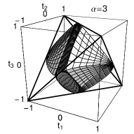
(b)
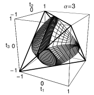
(c)

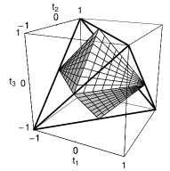
Figure 1: Comparison of inequality (2.21) and that proposed in Ref. Guhne in the case of Bell-diagonal states. In both upper figures (a) the region which satisfies our inequalities is presented (left for $\alpha=3$ and right for $\alpha=6$), while in figures (b) the states satisfying inequalities from Ref. Guhne are shown (for the same values of $\alpha$). For comparison in figure (c) the tetrahedron of all the Bell-diagonal states and octahedron containing Bell-diagonal separable states are displayed MHRH .

The second class are the two-parameter states considered in Ref. DiV :

$$\tilde{\varrho}(b,c)=a\sum_{i=0}^{1}|ii\rangle\langle ii|+b|\psi_{-}\rangle\langle\psi_{-}|+c|\psi_{+}\rangle\langle\psi_{+}|,$$ (2.29)

where $|\psi_{\pm}\rangle$ are defined as previously and $a=(1/2)(1-b-c)$. One can easily check that $\mathrm{Tr}_{B}\tilde{\varrho}(b,c)=\mathrm{Tr}_{A}\tilde{\varrho}(b,c)=(1/2)\mathbbm{1}_{2}$ and the assumption of Fact 1 is satisfied. Comparison with the entropic inequalities for $\alpha=3$ and $\alpha=5$ is shown in Fig. 2.

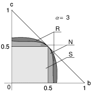
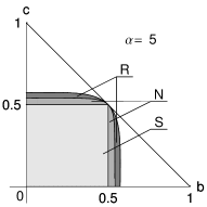
Figure 2: The comparison of entropic inequalities and the present ones in the case of states given by (2.29). The triangle specifies the range of parameters $b$ and $c$ for which Eq. (2.29) represents a state. Square $S$ denotes a subset of separable states. States which are not detected by standard entropic inequalities are represented by darker gray set marked with $R$, while the brighter gray set marked with $N$ indicates the states which are not detected by the inequality (2.21). The sets overlap in the region near separable states (i.e., $S\subset N\subset R$). From the analysis one concludes that the set of entangled states detected by our inequalities is considerably bigger than the set corresponding to entropic inequalities. Plots are made for $\alpha=3$ and $\alpha=5$.

2.2 General scalar inequalities.

In the paragraph we generalize the above results to bipartite systems with arbitrarily dimensional subsystems. The property $\mathbbm{1}_{2}\otimes\varrho_{B}=\varrho+\varrho^{\tau_{A}}$ possessed by states on the Hilbert space $\mathbb{C}^{2}\otimes\mathbb{C}^{d}$ is in general not valid for systems defined on $\mathbb{C}^{d_{A}}\otimes\mathbb{C}^{d_{B}}$. However, the separability criterion based on the general map $\Lambda_{U}^{(-)}$ provides us with the operator inequalities $\varrho_{A}\otimes\mathbbm{1}_{d_{B}}\geq\varrho+\varrho^{\tau_{B}^{U}}$ and $\mathbbm{1}_{d_{A}}\otimes\varrho_{B}\geq\varrho+\varrho^{\tau_{A}^{U}}$, which are true for an arbitrary bipartite separable state. In the following fact we propose an inequality resulting from the Breuer-Hall map.

Fact 2. If a given state $\varrho$ on $\mathbb{C}^{d_{A}}\otimes\mathbb{C}^{d_{B}}$ is separable and has the property that $[\varrho,\varrho_{A}\otimes\mathbbm{1}_{d_{B}}]=0$ $([\varrho,\mathbbm{1}_{d_{A}}\otimes\varrho_{B}]=0)$ then for an arbitrary natural number $\alpha\geq 1$ footnote2

$$\mathrm{Tr}\varrho_{A(B)}^{\alpha}\geq\mathrm{Tr}\varrho\left(\varrho+\varrho^{\tau_{B(A)}^{U}}\right)^{\alpha-1}.$$ (2.30)

Proof. The proof is a simple consequence of few well known facts. Let $\varrho$ be a state obeying the assumptions of the theorem. Then, since in general

$$[\varrho,\varrho_{A}\otimes\mathbbm{1}_{d_{B}}]^{\tau_{B}^{U}}=[\varrho^{\tau_{B}^{U}},\varrho_{A}\otimes\mathbbm{1}_{d_{B}}],$$ (2.31)

the assumption $[\varrho,\varrho_{A}\otimes\mathbbm{1}_{d_{B}}]=0$ implies that also $[\varrho^{\tau_{B}^{U}},\varrho_{A}\otimes\mathbbm{1}_{d_{B}}]=0$. Therefore one has

$$\varrho_{A}^{\alpha-1}\otimes\mathbbm{1}_{d_{B}}=(\varrho_{A}\otimes\mathbbm{1}_{d_{B}})^{\alpha-1}\geq\left(\varrho+\varrho^{\tau_{B}^{U}}\right)^{\alpha-1}.$$ (2.32)

Exploiting the property that if $A\geq B$ then also $X^{\dagger}AX\geq X^{\dagger}BX$ for an arbitrary matrix $X$ we may write

$$\sqrt{\varrho}(\varrho_{A}\otimes\mathbbm{1}_{d_{B}})^{\alpha-1}\sqrt{\varrho}\geq\sqrt{\varrho}\left(\varrho+\varrho^{\tau_{B}^{U}}\right)^{\alpha-1}\sqrt{\varrho}.$$ (2.33)

Finally, since if $A\geq B$ then also $\mathrm{Tr}A\geq\mathrm{Tr}B$, we obtain the postulated inequality

$$\mathrm{Tr}\varrho(\varrho_{A}\otimes\mathbbm{1}_{d_{B}})^{\alpha-1}=\mathrm{Tr}\varrho_{A}^{\alpha}\geq\mathrm{Tr}\varrho\left(\varrho+\varrho^{\tau_{B}^{U}}\right)^{\alpha-1},$$ (2.34)

finishing the proof. $\square$

Remark 2.1. Assuming that $[\varrho_{A}\otimes\mathbbm{1}_{d_{B}},\varrho]=0$ the operator inequality in Eq. (2.32) itself may lead to a criterion detecting entanglement, which is stronger than the one for $\alpha=2$, i.e., following from the linear map. Analysis of these inequalities will be made in one of the next subsections.

Remark 2.2. Assuming again that $\varrho$ represents a separable state one has $\big{|}\varrho^{\tau_{A(B)}^{U}}\big{|}=\varrho^{\tau_{A(B)}^{U}}$ and therefore

$$\mathrm{Tr}\varrho_{A(B)}^{\alpha}\geq\mathrm{Tr}\varrho\left(\varrho+\left|\varrho^{\tau_{B(A)}^{U}}\right|\right)^{\alpha-1}.$$ (2.35)

This inequality is stronger than the previous one, however, since it contains an absolute value of a matrix, it is, to our knowledge, not measurable on few copies of state.

The generalization of Fact 1 to higher-dimensional states is also possible. Let us state it as the following fact.

Fact 3. Assume that $\varrho$ is a separable state acting on $\mathbb{C}^{d_{A}}\otimes\mathbb{C}^{d_{B}}$ and that the commutator $\big{[}\varrho,\mathbbm{1}_{d_{A}}\otimes\varrho_{B}\big{]}$ disappears, then for a natural number $\alpha\geq 1$

$$\mathrm{Tr}\varrho_{A}^{\alpha}\geq\frac{1}{2}\left[\mathrm{Tr}\varrho\left(\varrho+\varrho^{\tau_{B}^{U}}\right)^{\alpha-1}+\mathrm{Tr}\varrho\left(\varrho-\varrho^{\tau_{B}^{U}}\right)^{\alpha-1}\right].$$ (2.36)

Proof. Let us consider the map $\Lambda_{U}^{(+)}$ introduced at the beginning of the section, Eq. (2.3). It leads to the separability criterion $\mathbbm{1}_{d_{A}}\otimes\varrho_{B}\geq\varrho-\varrho^{\tau_{A}^{U}}$. Now, applying the methods used in the proof of Fact 2 to the criterion resulting from $\Lambda_{U}^{(+)}$ we obtain the following inequality

$$\mathrm{Tr}\varrho_{B}^{\alpha}\geq\mathrm{Tr}\varrho\left(\varrho-\varrho^{\tau_{A}^{U}}\right)^{\alpha-1},$$ (2.37)

which is fulfilled by all separable states satisfying the commutativity assumption. Combining the inequalities (2.30) and (2.37) we obtain the inequality (2.36). Note that the analogous inequality can be also derived for the second subsystem. 

Remark 3.1 For states $\varrho$ that commute with $\varrho^{\tau_{A}^{U}}$ (i.e. $\big{[}\varrho,\varrho^{\tau_{A}^{U}}\big{]}=0$) and for natural $\alpha\geq 2$ some terms on the right-hand side of the inequality (2.30) can be removed, leading to general inequalities of the form

$$\mathrm{Tr}\varrho_{A(B)}^{\alpha}\geq\mathrm{Tr}\varrho^{\alpha}+G_{\alpha}(\varrho),$$ (2.38)

where $G_{\alpha}(\varrho)$ is a sum of terms of type (2.10) such that the inequality remains true for all separable states. Note that the same procedure was proposed in the previous subsection. Since again, the above represents somehow improved entropic inequality it should, in principle, be more powerful, whenever $G_{\alpha}(\varrho)$ is positive for any entangled state $\varrho$. Note that the inequality proposed in Fact 3 is also of this form

It is interesting to analyze the limit $\alpha\to\infty$ for the inequality (2.36). It can be easily done since one assumes that $\big{[}\varrho,\varrho^{\tau_{A}^{U}}\big{]}=0$. Let us transform Eq. (2.36) to the following form

$$\frac{\log\mathrm{Tr}\varrho_{B}^{\alpha}}{1-\alpha}\leq\frac{\log\displaystyle\left\{\frac{1}{2}\mathrm{Tr}\varrho\left[\left(\varrho+\varrho^{\tau_{A}^{U}}\right)^{\alpha-1}+\left(\varrho-\varrho^{\tau_{A}^{U}}\right)^{\alpha-1}\right]\right\}}{1-\alpha}.$$ (2.39)

The left-hand side of the above inequality is the Renyi entropy of subsystem $\varrho_{B}$, and due to Ref. MHPH in the limit $\alpha\to\infty$ gives $-\log||\varrho_{B}||$, where $||\varrho_{B}||$ is an operator norm of $\varrho_{B}$. Due to the assumption that $\big{[}\varrho,\varrho^{\tau_{A}^{U}}\big{]}=0$, there exists a common orthonormal basis of eigenvectors of $\varrho$ and $\varrho^{\tau_{A}^{U}}$. We denote it by $\{|\psi_{i}\rangle\}$. Then $\varrho+\varrho^{\tau_{A}^{U}}$ and $\varrho-\varrho^{\tau_{A}^{U}}$ must have the same eigenvectors as $\varrho$.

Let $\lambda_{i}$, $\lambda_{i}^{\tau}$, $\lambda^{+}_{i}$, $\lambda^{-}_{i}$ denote the eigenvalues of $\varrho$, $\varrho^{\tau_{A}^{U}}$, $\varrho+\varrho^{\tau_{A}^{U}}$ and $\varrho-\varrho^{\tau_{A}^{U}}$, corresponding to eigenvector $|\psi_{i}\rangle$. We can than rewrite Eq. (2.39) as

$$\frac{\log\mathrm{Tr}\varrho_{B}^{\alpha}}{1-\alpha}\leq\frac{\log\left\{\displaystyle\frac{1}{2}\displaystyle\sum_{i}\lambda_{i}\left[(\lambda^{+}_{i})^{\alpha-1}+(\lambda^{-}_{i})^{\alpha-1}\right]\right\}}{1-\alpha}.$$ (2.40)

We need to show that the argument of logarithm is positive. Henceforward we will assume that all $\lambda_{i}$ are strictly positive since terms with $\lambda_{i}=0$ do not contribute to the sum under logarithm. Therefore one sees that

$$\sum_{i}\lambda_{i}\left[(\lambda^{+}_{i})^{\alpha-1}+(\lambda^{-}_{i})^{\alpha-1}\right]\geq 0$$ (2.41)

and since all terms in the sum are nonnegative the equality is possible only if $(\lambda^{+}_{i})^{\alpha-1}+(\lambda^{-}_{i})^{\alpha-1}=0$ for all $i$. This, however, is impossible since all such terms are of the form $(\lambda_{i}+\lambda_{i}^{\tau})^{k}+(\lambda_{i}-\lambda_{i}^{\tau})^{k}$ with $\lambda_{i}>0$ and $\lambda_{i}^{\tau}\geq 0$. Now the positivity can be seen by a straightforward calculation using the binomial formula.

We introduce the following notation $\lambda^{+}_{\mathrm{max}}=\max_{i}\{|\lambda_{i}^{+}|\}$, $\lambda^{-}_{\mathrm{max}}=\max_{i}\{|\lambda_{i}^{-}|\}$, remembering that we exclude the situation $\lambda_{i}=0$. So $\lambda^{\pm}_{\mathrm{max}}$ are the maximum eigenvalues of $|\varrho\pm\varrho^{\tau_{A}^{U}}|$ corresponding to a nonzero $\lambda_{i}$. By $q_{\max}$ we denote $\max\{\lambda^{+}_{\mathrm{max}},\lambda^{-}_{\mathrm{max}}\}$. Moreover, let $\tilde{\lambda}^{+}_{i}=\lambda^{+}_{i}/q_{\max}$ and $\tilde{\lambda}^{-}_{i}=\lambda^{-}_{i}/q_{\max}$. Now we may rewrite Eq. (2.40) as

$$\frac{\log\mathrm{Tr}\varrho_{B}^{\alpha}}{1-\alpha}\leq\frac{\log q_{\mathrm{max}}^{\alpha-1}}{1-\alpha}+\frac{\log\frac{1}{2}\left\{\displaystyle\sum_{i}\lambda_{i}\left[(\tilde{\lambda}^{+}_{i})^{\alpha-1}+(\tilde{\lambda}^{-}_{i})^{\alpha-1}\right]\right\}}{1-\alpha}$$ (2.42)

and finally as

$$\frac{\log\mathrm{Tr}\varrho_{B}^{\alpha}}{1-\alpha}\leq-\log q_{\mathrm{max}}+\frac{\log\frac{1}{2}\left\{\displaystyle\sum_{i}\lambda_{i}\left[(\tilde{\lambda}_{i}^{+})^{\alpha-1}+(\tilde{\lambda}_{i}^{-})^{\alpha-1}\right]\right\}}{1-\alpha}.$$ (2.43)

It should be mentioned that the logarithm in the second term on right-hand side of the above inequality is finite in the limit $\alpha\to\infty$ since $\sum_{i}\lambda_{i}\big{[}(\tilde{\lambda}_{i}^{+})^{\alpha-1}+(\tilde{\lambda}_{i}^{-})^{\alpha-1}\big{]}$ is bounded from above and can never approach zero when $\alpha\to\infty$.

Zero under logarithm can only come from a term such as $1^{\alpha}+(-1)^{\alpha}$ which is equivalent to $\lambda_{\mathrm{max}}^{+}=\lambda_{\mathrm{max}}^{-}$ and $\lambda_{i}^{-}=-\lambda_{\mathrm{max}}^{-}$ for some $i$ (let us denote this particular index by $N$). This, in turn, could happen only if $\lambda_{N}+\lambda_{N}^{\tau}=-(\lambda_{N}-\lambda_{N}^{\tau})$ leading to $\lambda_{N}=0$. Such situation, however, was excluded at the outset. Thus, one sees that the logarithm is always finite and taking the limit $\alpha\to\infty$ on both sides we obtain

$$-\log{||\varrho_{B}||}\leq-\log q_{\mathrm{max}},$$ (2.44)

which can be also written as

$$||\varrho_{B}||\geq\max\{\lambda_{\mathrm{max}}^{+},\lambda_{\mathrm{max}}^{-}\}.$$ (2.45)

A similar inequality one may derive for $\varrho_{A}$. Moreover, comparison with Eq. (1.8) shows that the just derived inequality must be stronger than its entropic counterpart. Let us now present the second inequality which is also based on Breuer-Hall map, however, its derivation is a little bit more involving.

Fact 4. Assume that $\varrho$ acting on $\mathbb{C}^{d_{A}}\otimes\mathbb{C}^{d_{B}}$ is separable and $[\varrho,\varrho^{\tau_{A(B)}^{U}}]=0$ with a given antisymmetric unitary $U$. Then for $\alpha>1$ the following inequality holds:

$$\mathrm{Tr}\varrho_{B(A)}^{\alpha}\geq 2^{\alpha-1}\left[\mathrm{Tr}\varrho^{\frac{\alpha+1}{2}}\left(\varrho^{\tau_{A(B)}^{U}}\right)^{\frac{\alpha-1}{2}}\right].$$ (2.46)

Proof. The proof goes along the same lines as presented in Ref. VollbrechtWolf . First we may write

$$\mathrm{Tr}\varrho_{B}^{\alpha}=\mathrm{Tr}\varrho(\mathbbm{1}_{d_{A}}\otimes\varrho_{B})^{\alpha-1}=\mathrm{Tr}e^{\log\varrho}e^{(\alpha-1)\log\mathbbm{1}_{d_{A}}\otimes\varrho_{B}}.$$ (2.47)

Now, since $\mathrm{Tr}\,e^{A}e^{B}\geq\mathrm{Tr}\,e^{A+B}$ (see Ref. Bhatia ) and due to the equation $\mathbbm{1}_{d_{A}}\otimes\varrho_{B}\geq\varrho+\varrho^{\tau_{A}^{U}}$ and monotonicity of the logarithm, we have

$$\mathrm{Tr}\varrho_{B}^{\alpha}\geq\mathrm{Tr}e^{\log\varrho+(\alpha-1)\log\big{(}\varrho+\varrho^{\tau_{A}^{U}}\big{)}}.$$ (2.48)

Then we may use concavity of the logarithm to obtain

$$\mathrm{Tr}\varrho_{B}^{\alpha}\geq 2^{\alpha-1}\mathrm{Tr}\,e^{[(\alpha+1)/2]\log\varrho+[(\alpha-1)/2]\log\varrho^{\tau_{A}^{U}}}.$$ (2.49)

Finally by virtue of the assumption that $\varrho$ and $\varrho^{\tau_{A}^{U}}$ commute we have the commutativity of their logarithms, and therefore

$$\mathrm{Tr}\varrho^{\alpha}_{B}\geq 2^{\alpha-1}\mathrm{Tr}\left[\varrho^{\frac{\alpha+1}{2}}\left(\varrho^{\tau_{A}^{U}}\right)^{\frac{\alpha-1}{2}}\right],$$ (2.50)

finishing the proof.

Remark 4.1. The remark here is that in the above inequality for $\alpha=2k$ one gets the square roots of $\varrho^{\tau_{A}^{U}}$, which in case of entangled states may lead to complex eigenvalues. Moreover, the inequality may be strengthened by taking only the even powers of $\varrho^{\tau_{A}^{U}}$, since in such case the RHS would remain positive even for entangled states. Therefore we assume that $\alpha=4k+1$. Then the inequality may be rewritten as

$$\mathrm{Tr}\varrho^{4k+1}_{B(A)}\geq 2^{4k}\mathrm{Tr}\left[\varrho^{2k+1}\left(\varrho^{\tau_{A(B)}^{U}}\right)^{2k}\right]\quad(k=0,1,\ldots).$$ (2.51)

Remark 4.2. If we take the values of $\alpha$ as in Remark 4.1., i.e. $\alpha_{k}=4k+1$ it is again possible to derive the inequality for $k\to\infty$. The reasoning is similar as in the limiting case of inequality (2.36). We take the logarithm of both sides of Eq. (2.46) and divide the inequality by $1-\alpha_{k}=-4k$ obtaining

$$\frac{\log\mathrm{Tr}\varrho_{B(A)}^{4k+1}}{-4k}\leq\frac{\log 2^{4k}\left[\mathrm{Tr}\varrho\left(\varrho\varrho^{\tau_{A(B)}^{U}}\right)^{2k}\right]}{-4k}.$$ (2.52)

It is easy to check that in the limit $k\to\infty$ after omitting the logarithm we obtain

$$||\varrho_{B}||\geq 2\sqrt{\left|\left|\varrho\varrho^{\tau_{A}^{U}}\right|\right|}.$$ (2.53)

Remark 4.3. In the case when $[\varrho_{A}\otimes\mathbbm{1}_{d_{B}},\varrho]\neq 0$, it is still possible to derive certain inequality detecting entanglement, however, most probably not measurable. To achieve this goal we use two facts. The first one says that for arbitrary matrices $A$ and $B$, the following equality

$$\lim_{m\to\infty}\left(e^{\frac{B}{2m}}e^{\frac{A}{m}}e^{\frac{B}{2m}}\right)^{m}=e^{A+B}.$$ (2.54)

holds (see Ref. Bhatia ). Therefore one sees that

$$e^{\frac{\alpha+1}{2}\log\varrho+\frac{\alpha-1}{2}\log\varrho^{\tau_{A}}}$$ (2.55)

$$\hskip 14.45377pt=\lim_{m\to\infty}\left(e^{\frac{\alpha+1}{4m}\log\varrho}e^{\frac{\alpha-1}{2m}\log\varrho^{\tau_{A}^{U}}}e^{\frac{\alpha+1}{4m}\log\varrho}\right)^{m}$$

$$\hskip 14.45377pt=\lim_{m\to\infty}\left(\varrho^{\frac{\alpha+1}{4m}}(\varrho^{\tau_{A}^{U}})^{\frac{\alpha-1}{2m}}\varrho^{\frac{\alpha+1}{4m}}\right)^{m}.$$ (2.56)

and by virtue of the continuity of the trace, we have

$$\mathrm{Tr}\varrho_{B}^{\alpha}\geq\lim_{m\to\infty}\mathrm{Tr}\left[\varrho^{\frac{\alpha+1}{4m}}\left(\varrho^{\tau_{A}^{U}}\right)^{\frac{\alpha-1}{2m}}\varrho^{\frac{\alpha+1}{4m}}\right]^{m}.$$ (2.57)

As the second fact we make use of the inequality Lieb :

$$\mathrm{Tr}\left[B^{r}(\sqrt{B}A\sqrt{B})^{s}\right]\geq\mathrm{Tr}\left[\left(\Sigma_{\uparrow}(A))^{s}(\Sigma_{\downarrow}(B)\right)^{r+s}\right],$$ (2.58)

where $A$ and $B$ are positive $n\times n$ matrices, $r\geq 0$, and $s\geq 1$. Here, $\Sigma_{\uparrow}(A)$ and $\Sigma_{\downarrow}(A)$ are defined as

$$\Sigma_{\uparrow}(A)=\left(\begin{array}[]{cccc}\sigma_{1}&0&\ldots&0\\ 0&\sigma_{2}&\ldots&0\\ \vdots&\vdots&\ddots&\vdots\\ 0&0&\ldots&\sigma_{n}\end{array}\right)$$ (2.59)

and

$$\Sigma_{\downarrow}(A)=\left(\begin{array}[]{cccc}\sigma_{n}&0&\ldots&0\\ 0&\sigma_{n-1}&\ldots&0\\ \vdots&\vdots&\ddots&\vdots\\ 0&0&\ldots&\sigma_{1}\end{array}\right),$$ (2.60)

where $\sigma_{1}\geq\sigma_{2}\geq\ldots\geq\sigma_{n}$ are singular values of $A$, i.e., eigenvalues of $|A|=\sqrt{A^{\dagger}A}$.

Substituting $r=0,\;s=m$ and $\sqrt{B}=\varrho^{(\alpha+1)/4m}$, and $A=(\varrho^{\tau_{A}^{U}})^{(\alpha-1)/2m}$ to Eq. (2.58), one arrives at

$$\mathrm{Tr}\varrho_{B}^{\alpha}\geq\lim_{m\to\infty}\mathrm{Tr}\left\{\left[\Sigma_{\uparrow}\big{(}(\varrho^{\tau_{A}^{U}})^{\frac{\alpha-1}{2m}}\big{)}\right]^{m}\left[\Sigma_{\downarrow}\big{(}\varrho^{\frac{\alpha+1}{2m}}\big{)}\right]^{m}\right\}.$$ (2.61)

Moreover, in the case of Hermitian $A$ one has $\Sigma_{\uparrow}(A^{k})=(\Sigma_{\uparrow}(A))^{k}$, which in turn allows us to write

$$\mathrm{Tr}\varrho_{B}^{\alpha} \geq \lim_{m\to\infty}\mathrm{Tr}\left[(\Sigma_{\uparrow}(\varrho^{\tau_{A}^{U}}))^{\frac{\alpha-1}{2}}(\Sigma_{\downarrow}(\varrho))^{\frac{\alpha+1}{2}}\right]$$ (2.62)

$$= \mathrm{Tr}\left[\big{(}\Sigma_{\uparrow}(\varrho^{\tau_{A}^{U}})\big{)}^{\frac{\alpha-1}{2}}\big{(}\Sigma_{\downarrow}(\varrho)\big{)}^{\frac{\alpha+1}{2}}\right].$$

Since for a density matrix $|\varrho|=\varrho$ the singular values of $\varrho$ are just its eigenvalues.

2.3 Operator inequalities.

In the proof of Fact 2 we considered an operator inequality given by Eq. (2.32). As we will see below this operator inequality is interesting to be analyzed itself. Namely, assuming that a given $\varrho$ on $\mathbb{C}^{d_{A}}\otimes\mathbb{C}^{d_{B}}$ is separable and obeys $[\varrho,\varrho_{A}\otimes\mathbbm{1}_{d_{B}}]=0$, then

$$(\varrho_{A}\otimes\mathbbm{1}_{d_{B}})^{\alpha}\geq\left(\varrho+\varrho^{\tau_{B}^{U}}\right)^{\alpha},$$ (2.63)

for natural $\alpha\geq 1$. Equivalently, under the assumption that $[\varrho,\mathbbm{1}_{d_{A}}\otimes\varrho_{B}]=0$, we get the dual inequality of the form

$$(\mathbbm{1}_{d_{A}}\otimes\varrho_{B})^{\alpha}\geq\left(\varrho+\varrho^{\tau_{A}^{U}}\right)^{\alpha}.$$ (2.64)

Both inequalities are an immediate consequences of the fact that if $[A,B]=0$ then $A\geq B\geq 0$ implies $A^{\alpha}\geq B^{\alpha}$ for real $\alpha>0$.

For states that commute with $\varrho^{\tau^{U}_{B}}$ (i.e., $[\varrho,\varrho^{\tau_{B}^{U}}]=0$), the inequality (2.63) gives rise to the family of inequalities of the form

$$(\varrho_{A}\otimes\mathbbm{1}_{d_{B}})^{\alpha}\geq\varrho^{\alpha}+\mathcal{G}_{\alpha}(\varrho),$$ (2.65)

where $\mathcal{G}_{\alpha}(\varrho)$ denotes a linear combination of products of different powers of $\varrho$ and $\varrho^{\tau_{B}^{U}}$. The operator $\mathcal{G}_{\alpha}(\varrho)$ obviously depends on parameter $\alpha$ and is obtained by removing some positive terms on the RHS of the inequality (2.63).

An example of inequality of the type (2.65) is

$$(\varrho_{A}\otimes\mathbbm{1}_{d_{B}})^{\alpha} \geq \left(\varrho+\varrho^{\tau_{B}^{U}}\right)^{\alpha}$$ (2.66)

$$\geq \frac{1}{2}\left[\left(\varrho+\varrho^{\tau_{B}^{U}}\right)^{\alpha}+\left(\varrho-\varrho^{\tau_{B}^{U}}\right)^{\alpha}\right],$$

where the terms with odd powers of $\varrho^{\tau_{B}^{U}}$ has been removed, since for separable states $\varrho^{m}\big{(}\varrho^{\tau_{B}^{U}}\big{)}^{n}\geq 0$ for all $m,\,n\geq 1$. This is the operator version of the scalar inequality proposed in Fact 3. Again, it is enough to assume that $\big{[}\varrho,\varrho_{A}\otimes\mathbbm{1}\big{]}$. It may be rewritten in the form

$$(\varrho_{A}\otimes\mathbbm{1}_{d_{B}})^{\alpha}\geq\varrho^{\alpha}+\sum_{k=1}^{\lfloor\alpha/2\rfloor}\varrho^{\alpha-2k}\left(\varrho^{\tau_{B}^{U}}\right)^{2k}.$$ (2.67)

One should notice, that if the state $\varrho$ has negative partial time reversal then the removed terms could become nonpositive and removing them from Eq. (2.63) should make the inequality more powerful than the Breuer criterion. The comparison to Breuer criterion and others is presented in the next section.

2.4 Comparison

We shall now compare the scalar inequalities and the operator inequality introduced in previous paragraphs with the known scalar and structural separability criteria, paying particular attention to the entropic inequalities and the criterion formulated by Breuer Bcrit . The large class of states that possesses all the features necessary to apply the inequalities derived in previous sections are the rotationally invariant bipartite states (for some results on separability properties of $\mathrm{SO}(3)$-invariant states see Refs. rot ; RAJS ). They have maximally mixed subsystems and their partial time reversal with respect to arbitrary subsystem does not change the eigenvectors of a state, so they fulfil the assumption $[\varrho,\varrho^{\tau_{A(B)}}]=0$. Every bipartite $\mathrm{SO}(3)$-invariant state with subsystems of spin $j_{1}$ and $j_{2}$ such that $j_{1}\leq j_{2}$ can be written in the basis of projections on eigenspaces of total angular momentum $P_{J}$, where $J=|j_{1}-j_{2}|,\ldots,j_{1}+j_{2}$, i.e.,

$$\varrho=\sum_{J=|j_{1}-j_{2}|}^{j_{1}+j_{2}}\alpha_{J}P_{J}.$$ (2.68)

Normalization is such that $\mathrm{Tr}P_{J}=1$.

We shall focus our attention on the case of $4\otimes 4$ states for which entanglement is fully characterized by partial transposition and Breuer’s map, i.e., Breuer criterion in this case detects all bound entangled states. Each state depends on three nonnegative parameters $p$, $q$, $r$ such that $0\leq 1-p-q-r\leq 1$ and can be written as

$$\varrho(p,q,r)=pP_{0}+qP_{1}+rP_{2}+(1-p-q-r)P_{3}.$$ (2.69)

We start the analysis with comparing the new inequalities (2.36) and (2.46) with standard entropic ones. As shown in Fig. 3 the set of states that fulfil the entropic inequality is much larger than these for the present inequalities. Thus the scalar criteria (2.36) and (2.46) resulting from the extended reduction map are indeed much stronger than the entropic ones, since for the same values of $\alpha$ they detect more entangled states (regions outside the respective sets). Moreover the significant feature of the derived inequalities is that they detect PPT entangled states. However, in the limit $\alpha\to\infty$ the inequality (2.36) detects all bound entangled states, whereas inequality (2.46) only some part of the set.

(a)
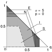
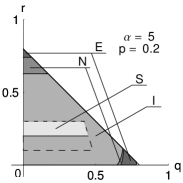
(b)

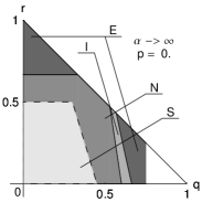
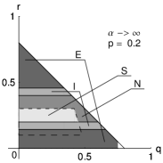
Figure 3: The comparison of entropic inequalities with these derived in the present paper for $\alpha=5$, (a) and $\alpha\to\infty$, (b) and state parameter $p=0$ and $p=0.2$. The range of parameters $q,r$ that represent a state for given $p$ is the triangle marked in each picture. The sets for which the respective inequalities are fulfilled overlap in the area around the separable states and therefore only some parts of them are visible in the pictures. To avoid confusion the sets are marked both with colors and letters. The largest, $E$, the set for which the $\alpha$-entropic inequality is fulfilled, $N$, inequality (2.36), $I$, inequality (2.46) and the smallest $S$, the set of separable states. The dashed line is the border of the set of PPT states.

In Figs. 4 and 5 the effectiveness of the inequalities proposed in the paper is shown. The comparison of inequalities (2.35) and (2.36) is made in Fig. 4. It can be seen that the second is stronger than the first one, i.e., detects more entangled states for the same value of parameter $\alpha$. Comparing the figures in the right column one can see how the PPT entangled states are detected with the growth of parameter $\alpha$. In the limit $\alpha\to\infty$ (marked in each figure with $L$) both inequalities detect the whole set of bound entangled states.

(a)
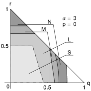
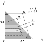
(b)
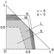
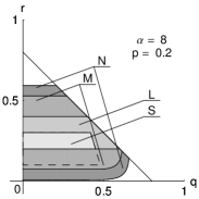
(c)

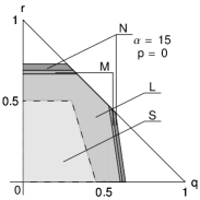
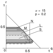
Figure 4: The comparison of inequalities (2.36) and (2.35) for $\alpha=3$ (a), $\alpha=8$ (b), and $\alpha=15$ (c) and state parameter $p=0$ and $p=0.2$. The set of parameters $q,r$ which represent a state for given $p$ is the triangle marked in each figure. Sets for which respective inequalities are fulfilled overlap in the region surrounding the set of separable states S (i.e., $S\subset L\subset M\subset N$). We mark them as follows, $N$, states that fulfil Eq. (2.36), $M$, Eq. (2.35), $L$, the limit $\alpha\to\infty$ of Eqs. (2.36) and (2.35). The dashed line is the border of the set of PPT states.

The effectiveness of Eq. (2.51) is shown in Fig. 5. The set marked with $I$ converges to the one marked by $L$ with the growing $\alpha$. It should be noticed that even for relatively small values of $\alpha$ the difference between the sets $I$ and $L$ is small.

(a)
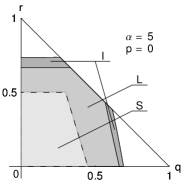
(b)

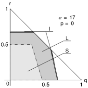
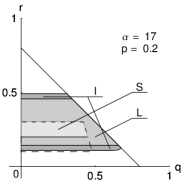
Figure 5: The set of states that fulfil the Eq. (2.46) is marked with $I$, the limiting case $\alpha\to\infty$ of this inequality is denoted by $L$. Again $S$ denotes the set of separable states and the dashed line the border of the set of PPT states. ($S\subset L\subset I$) The triangle is the set of parameters $q,r$ which represent a state. The figures are made for two values of state parameter $p=0$ and $p=0.2$ and $\alpha=5$ (a), $\alpha=17$ (b).

In Fig. 6 we compare the operator inequality (2.66) derived in the previous section with the positive map criterion proposed by Breuer. The figures contain also the scalar inequality (2.36) since it may be considered as a scalar analog of (2.66). It is clearly seen that the operator inequality (2.66), though arising from the Breuer’s map, detects some entanglement where the Breuer’s map fails. The scalar inequality is weaker than the operator one, however, in the limit $\alpha\to\infty$ both criteria are equivalent for this class of states.

(a)
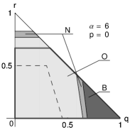
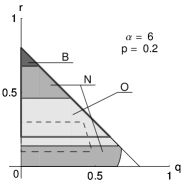
(b)

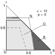
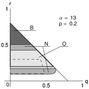
Figure 6: The comparison of operator inequality (2.66) with the scalar inequality (2.36) and the Breuer map criterion for $\alpha=6$ (a) and $\alpha=13$ (b). The set of parameters $q,r$ which represent a state for $p=0$ and $p=0.2$ is the triangle marked in each figure. Sets for which respective inequalities are fulfilled are marked as follows, $B$, the set of states that remain positive after the action of Breuer’s map, the borders of the set are marked with the thick gray line since the set is partially covered by other sets. $O$, states that fulfil Eq. (2.66), $N$, states that fulfil Eq. (2.36). The dashed line is the border of the set of PPT states. The set of separable states is the intersection of $B$ and the set of PPT states.

3 Multi-copy entanglement witnesses.

Here we discuss the applicability of just introduced scalar inequalities for construction of multicopy entanglement witnesses. One knows that measuring such observables may provide more information about entanglement of a given $\varrho$ than witnesses defined on a single copy. In particular, recently two-copy entanglement witnesses were shown to be a lower bound for concurrence of $\varrho$ Mintert .

First, the notions of the $n$-copy observable and $n$-copy entanglement witness were proposed in Ref. PH3 . The latter are Hermitian operators $\mathscr{W}^{(n)}$ such that their mean value on $n$ copies of any separable state $\varrho$ is positive and there exists an entangled state for which this mean value is negative. An example of such operator unambiguously determining whether the state is entangled was provided in Ref. RAPHMD for any two-qubit state and in Ref. RAJS for $2\otimes d$ rotationally invariant states with odd $d$.

Below we will show how the scalar inequalities considered in the present paper can be reformulated in terms of a single collective witness. First we present the general multicopy approach to entanglement tests in both scalar (based on witnesses) and structural (based on maps) scenarios. Consider the scalar inequalities provided in Secs. 2.1 and 2.2. They are all of the form

$$\mathrm{Tr}\left(\sum_{i=1}^{m}\mu_{i}\prod_{j=1}^{\alpha}\Theta_{ij}(\varrho)\right)\geq 0$$ (3.1)

for some linear maps $\Theta_{ij}$ that preserve Hermiticity and coefficients $\mu_{i}\in\mathbb{R}$. For instance, the inequality given by Eq. (2.36) has this form if $m=3$ and

$$\Theta_{1j} = \mathrm{Tr}_{B}\qquad\quad\,(j=1,\ldots,\alpha),$$

$$\Theta_{21} = \Theta_{31}=I,\quad$$

$$\Theta_{2j} = I+\tau_{B}^{U}\qquad(j=2,\ldots,\alpha),$$

$$\Theta_{3j} = I-\tau_{B}^{U}\qquad(j=2,\ldots,\alpha),$$ (3.2)

$\mu_{1}=1,\,\mu_{2}=\mu_{3}=-1/2$, $I$ is an identity map, and $\mathrm{Tr}_{B}$ denotes the partial trace over the second subsystem.

Now, assuming that $\mathrm{Tr}[\Pi_{j}\Theta_{ij}(\varrho)]\in\mathbb{R}$ for all $i$, we provide multicopy entanglement witnesses that follow from the above scalar inequalities and go beyond these provided for entropic inequalities PH3 . First, let us denote by $\mathscr{V}^{(n)}$ the $n$-copy swap operator

$$\mathscr{V}^{(n)}|\Phi_{1}\rangle|\Phi_{2}\rangle\ldots|\Phi_{n}\rangle=|\Phi_{n}\rangle|\Phi_{1}\rangle\ldots|\Phi_{n-1}\rangle,$$ (3.3)

which is a straightforward multipartite generalization of $\mathscr{V}^{(2)}$ introduced in Sec. 2.1. It has the property that

$$\mathrm{Tr}(\mathscr{V}^{(n)}\varrho_{1}\otimes\ldots\otimes\varrho_{n})=\mathrm{Tr}(\varrho_{1}\ldots\varrho_{n}).$$ (3.4)

However, one should notice that

$$\mathrm{Tr}(\mathscr{V}^{(n)\dagger}\varrho_{1}\otimes\ldots\otimes\varrho_{n})=\mathrm{Tr}(\varrho_{n}\ldots\varrho_{1}),$$ (3.5)

which is not the same as in Eq. (3.4). The equivalence between these two formulas exist only if both traces are real.

One can see that $\mathscr{V}^{(n)}$ is not a Hermitian operator and as such it cannot be treated as an observable. However, instead of $\mathscr{V}^{(n)}$ one may consider its Hermitian counterpart

$$\tilde{\mathscr{V}}^{(n)}=\frac{1}{2}\left(\mathscr{V}^{(n)}+\mathscr{V}^{(n)\dagger}\right),$$ (3.6)

of which the mean value on $n$ copies of the state $\varrho$ gives exactly $\mathrm{Tr}\varrho^{n}$. Now, to take into account the maps in the formula (3.1), we use approach exploited already in case of positive maps method PHRAMD and define the following collective witness:

$$\mathscr{W}^{(\alpha)}=\sum_{i=1}^{m}\mu_{i}\left(\bigotimes_{j=1}^{\alpha}\Theta_{ij}^{\dagger}\right)\left(\tilde{\mathscr{V}}^{(\alpha)}\right)$$ (3.7)

which is Hermitian by the construction. Here by $\Theta^{\dagger}$ we denote a dual map of $\Theta$, i.e., the map obeying $\mathrm{Tr}[X\Theta(Y)]=\mathrm{Tr}[\Theta^{\dagger}(X)Y]$ for all matrices $X$ and $Y$.

Then the collective witness inequality that is equivalent to Eq. (3.1) is of the form

$$\mathrm{Tr}(\mathscr{W}^{(\alpha)}\varrho^{\otimes\alpha})\geq 0.$$ (3.8)

As illustrative examples we consider witnesses following from inequalities given by Eq. (2.36) and the ones given by Eq. (2.51). In the first case one needs to take dual maps $\Theta^{\dagger}_{ij}$ $(i=1,2,3,\;j=1,\ldots,\alpha)$ of the ones defined by Eq. (3). In the second case one takes $\Theta_{1j}$ for $j=1,\ldots,4k+1$ as defined in the previous case and

$$\Theta_{2j}=I\quad\quad(j=1,\ldots,2k+1),$$

$$\Theta_{2j}=\tau_{A(B)}^{U}\quad(j=2k+2,\ldots,4k+1),$$

$$\mu_{1}=1,\quad\mu_{2}=-2^{4k}.$$ (3.9)

Now we come back to operator inequalities of the type proposed in the Sec. 2.3. They are all of the form

$$\sum_{i=1}^{m}\mu_{i}\prod_{j=1}^{\alpha}\Theta_{ij}(\varrho)\geq 0,$$ (3.10)

where again $\Theta_{ij}$ are Hermiticity-preserving linear maps. Here we shall proceed in a slightly different way to highlight the analogy to positive maps separability condition. Namely, we can define the linear, map $\Lambda^{(n)}:{\cal H}_{AB}^{\otimes n}\rightarrow{\cal H}_{AB}$ by the formula

$$\Lambda^{(n)}(\cdot)=\sum_{k,m,i_{1},\ldots,i_{n}}P_{km}\mathrm{Tr}[P_{ki_{1}}\otimes P_{i_{1}i_{2}}\otimes P_{i_{2}i_{3}}\otimes\ldots\otimes P_{i_{n}m}(\cdot)]$$ (3.11)

with $P_{ij}=|i\rangle\langle j|$. The above map satisfies $\Lambda^{(\alpha)}(A_{1}\otimes A_{2}\otimes\ldots\otimes A_{\alpha})=A_{1}A_{2}\ldots A_{\alpha}$ for any operators $A_{i}$. Using the above map we can define the map

$$\Theta^{(\alpha)}=\Lambda^{(\alpha)}\circ\sum_{i=1}^{m}\mu_{i}\bigotimes_{j=1}^{n}\Theta_{ij}$$ (3.12)

and then the operator inequality (3.10) looks as follows

$$\Theta^{(\alpha)}(\varrho^{\otimes\alpha})\geq 0.$$ (3.13)

Since this inequality is satisfied iff $\langle\Psi|\Theta^{(\alpha)}(\varrho^{\otimes\alpha})|\Psi\rangle\geq 0$ for any vector $|\Psi\rangle$, we can immediately provide infinite set of $n$-copy entanglement witnesses

$$\mathscr{W}_{\Psi}^{(\alpha)}\equiv\Theta^{(\alpha)\dagger}(|\Psi\rangle\langle\Psi|).$$ (3.14)

4 Special inequality with the reflection map and its representation in terms of experimental quantities

4.1 Quadratic inequality based on reflection

Following the PPT test it is immediate to see that the following inequality is satisfied for any separable state

$$\mathrm{Tr}\left(\varrho\varrho^{\tau^{U}_{A(B)}}\right)\geq 0,$$ (4.1)

The above condition is related to the entropic inequality (1.6) by Eq. (2.30) (both taken with $\alpha=2$)

$$\mathrm{Tr}\varrho_{A(B)}^{2}-\mathrm{Tr}\varrho^{2}\geq\mathrm{Tr}\left(\varrho\varrho^{\tau_{B(A)}^{U}}\right).$$ (4.2)

So whenever this inequality is fulfilled (this is the case for some entangled states) Eq. (4.1) may be violated independently of respective entropic inequality. The effectiveness of inequalities in case of rotationally invariant states considered in Sec. 2.4 is presented in Fig. 7.

(a)
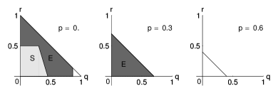
(b)

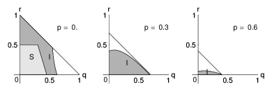
Figure 7: The comparison of the entropic inequalities (1.4) for $\alpha=2$ and $\mathrm{Tr}(\varrho\varrho^{\tau_{A(B)}})\geq{0}$ for $4\otimes 4$ rotationally invariant states (2.69). In all figures the light gray area marked with $S$ represents separable states. (a) The set of states that fulfill the entropic inequality $\mathrm{Tr}\varrho_{A(B)}^{2}-\mathrm{Tr}\varrho^{2}\geq 0$ (dark gray region marked with $E$). (b) The set of states that fulfill the inequality $\mathrm{Tr}(\varrho\varrho^{\tau_{A(B)}})\geq 0$ (dark gray region marked with $I$). The range of parameters $q$ and $r$ which represent the state for $p=0$, $p=0.3$, and $p=0.6$ is the triangle marked in all the figures.

Below we shall consider experimental detectability of the inequality (4.1) in case of the bipartite systems simulated by multiqubit ones.

4.2 Experimental detection of $\varrho\varrho^{\tau}$ for multiqubit systems

Consider an arbitrary state of $n$ qubits $\varrho_{A_{1}\ldots A_{n}}$. By the map $\tau_{i_{0}}$ we shall denote the reflection of $i_{0}$-th qubit on a Bloch sphere, i.e.,

$$\tau_{i_{0}}(\varrho_{A_{1},\ldots,A_{n}})=\mathbbm{1}_{n\setminus i_{0}}\otimes\sigma_{y}^{A_{i_{0}}}\varrho_{A_{1},\ldots,A_{n}}^{\Gamma_{i_{0}}}\mathbbm{1}_{n\setminus i_{0}}\otimes\sigma_{y}^{A_{i_{0}}},$$ (4.3)

where $\mathbbm{1}_{n\setminus i_{0}}$ means an identity acting on all parties excluding the $i_{0}$th one and $\Gamma_{i_{0}}$ denotes the partial transposition taken with respect to the $i_{0}$th particle. Since for any $i,j$ the maps $\tau_{i}$, $\tau_{j}$ commute, it makes sense to define for any set of increasing indices footnote3 $I^{\prime}=\{i_{1},\ldots,i_{k}\}$ the map

$$\tau_{i_{1},\ldots,i_{k}}(\cdot)=\tau_{i_{1}}\circ\ldots\circ\tau_{i_{k}}(\cdot)=(\cdot)^{\tau_{I^{\prime}}}.$$ (4.4)

The latter notation will be used subsequently. Now we are interested in general in measuring the following quantity

$$\mathrm{Tr}(\varrho\varrho^{\tau_{I^{\prime}}}).$$ (4.5)

It may be a little bit surprising that for two-qubit photon polarization state $\varrho$ the above quantity can be measured with virtually the same setup as in Ref. Bovino . It consists of two sources of pairs of photons and performs joint measurements on their polarization degrees of freedom. First source emits photons $A$ and $B$, the second one $A^{\prime}$ and $B^{\prime}$. Then the photons $A$ and $A^{\prime}$ ($B$ and $B^{\prime}$, respectively) meet at the beam splitter on Alice (Bob) side. Further, one measures whether they went out of the beam splitter together (coalescence) or not (anticoalescence) which formally corresponds to projection of two photon polarization state onto symmetric or antisymmetric (singlet) subspace. Since this happens on both Alice and Bob side the setup finally allows one to measure joint probabilities (corresponding to coalescence-coalescence, coalescence-anticoalescence, anticoalescence-coalescence and anticoalescence-anticoalescence). For $n$ qubits the direct generalization of the latter experiment (mathematics of which was considered in Ref. AlvesBosons ) also happens to work. The essential difference lies in the way, in which one has to combine the probabilities that come out from the experiment. Let us derive the probabilistic formula for the quantity (4.1). Consider the following collective two-copy multiqubit entanglement witness

$$W^{(2)}_{I^{\prime}}=\bigotimes_{i\in I\setminus I^{\prime}}\mathscr{V}^{(2)}_{A_{i}A^{\prime}_{i}}\bigotimes_{k\in I^{\prime}}P^{(-)}_{A_{k}A^{\prime}_{k}}.$$ (4.6)

Here $\mathscr{V}^{(2)}$ is a two-partite swap operator as defined in Eq. (3.3) and $P^{(-)}=(1/2)(\mathbbm{1}-\mathscr{V}^{(2)})$ is the antysymmetric projector, which is essentially the projector onto the singlet state $|\psi_{-}\rangle$. Let us recall that the subset of indices $I^{\prime}$ enumerates the qubits, on which the reflection in the second copy is to be performed. We have explicitly put the dependence of the observable on that set of indices.

After a little bit of algebra we get that our quantity (4.1) is reproduced as collective mean value of the observable

$$\big{\langle}\big{\langle}W^{(2)}_{I^{\prime}}\big{\rangle}\big{\rangle}_{\varrho}\equiv\mathrm{Tr}(W^{(2)}_{I^{\prime}}\varrho\otimes\varrho)=\mathrm{Tr}(\varrho\varrho^{\tau_{I^{\prime}}}).$$ (4.7)

Note that this quantity is closely related to entropic inequalities on multipartite qubits considered in Ref. AlvesBosons (which are natural generalizations of original entropic inequalities HHHEntr ) as well as to multipartite concurrences MintertMulti or other state functions based on nonlinear operations Osterloh .

Now there is a question how to measure the mean value of $W^{(2)}_{I^{\prime}}$. Consider the generalization of the scheme Bovino in a spirit of Ref. AlvesBosons . In this case on each pair of qubits $A_{i}A^{\prime}_{i}$ $(i=1,\ldots,n)$ one performs the measurement projecting onto one of two projectors, i.e., symmetric or antisymmetric one $P^{(\pm)}=(1/2)(\mathbbm{1}\pm\mathscr{V}^{(2)})$. For simplicity we shall denote the symmetric and antysymmetric projector by slightly different notations $P^{(0)}$ and $P^{(1)}$, respectively (note that the index is even or odd when the symmetry is even or odd).

With help of this notation let us denote the joint probabilities resulting in the experiment by

$$p(s_{1},\ldots,s_{n})=\mathrm{Tr}\left(\bigotimes_{j=1}^{n}P^{(s_{j})}_{A_{j}A^{\prime}_{j}}\varrho_{A_{1}\ldots A_{n}}\otimes\varrho_{A^{\prime}_{1}\ldots A^{\prime}_{n}}\right),$$ (4.8)

where $s_{i}\in\{0,1\}$. Now we derive the mean value of the observable (4.6). Let us define the characteristic function $\chi_{I^{\prime}}$ of a set of indices $I^{\prime}$ in a standard way, i.e., $\chi_{I^{\prime}}(i)=1$ if $i\in I^{\prime}$ and zero otherwise. Let us also introduce the function $\tilde{\chi}(s_{i})\equiv\chi_{I^{\prime}}(i)\delta_{s_{i},1}+\chi_{I\setminus I^{\prime}}(i)$. Then the mean value of the observable (4.6) is

$$\big{\langle}\big{\langle}W^{(2)}_{I^{\prime}}\big{\rangle}\big{\rangle}_{\varrho} = \sum_{s_{1},\ldots,s_{n}}(-1)^{\sum_{i}s_{i}\chi_{I\setminus I^{\prime}}(i)}\left[\tilde{\chi}(s_{1})\ldots\tilde{\chi}(s_{n})\right]$$ (4.9)

$$\times p(s_{1},\ldots,s_{n}).$$

The above complicated-looking formula has a very elementary interpretation. In fact we are summing only over such $s_{i}$ that have index $i\notin I^{\prime}$ and only they contribute to the ”phase” in the sum. All the indices $s_{i}$ with $i\in I^{\prime}$ are put to be one all the time. This can be easily seen in the following examples.

Example 1. Consider three qubits $(n=3)$ with the last one reflected $(I^{\prime}=\{3\})$. Then the last index in the probability is fixed to be one while the others are counted. This gives

$$\big{\langle}\big{\langle}W^{(2)}_{\{3\}}\big{\rangle}\big{\rangle}_{\varrho}=\sum_{i,j=0}^{1}(-1)^{i+j}p(i,j,1)=p(0,0,1)-p(0,1,1)$$

$$\hskip 39.83368pt-p(1,0,1)+p(1,1,1).$$ (4.10)

Now we introduce further examples that will have important interpretation in the context of bipartite systems.

Example 2. Consider again three qubits $(n=3)$ with last two reflected $(I^{\prime}=\{2,3\})$. This gives the very easy formula

$$\big{\langle}\big{\langle}W^{(2)}_{\{2,3\}}\big{\rangle}\big{\rangle}_{\varrho}=\sum_{i=0}^{1}(-1)^{i}p(i,1,1)=p(0,1,1)-p(1,1,1).$$ (4.11)

Example 3. Here we shall focus on four qubits $(n=4)$ and reflect the last two $(I^{\prime}=\{3,4\})$. The corresponding formula is

$$\big{\langle}\big{\langle}W^{(2)}_{\{3,4\}}\big{\rangle}\big{\rangle}_{\varrho}=\sum_{i,j=0}^{1}(-1)^{i+j}p(i,j,1,1)=p(0,0,1,1)$$

$$-p(0,1,1,1)-p(1,0,1,1)+p(1,1,1,1).$$ (4.12)

4.3 Application to bipartite systems of higher dimensions

Higher-dimensional bipartite systems, i.e., $d_{A}\otimes d_{B}$ with $d_{A}d_{B}>6$ behave in general much different than low-dimensional ones ($MN\leq 6$). In Sec. 4.1 we have seen this from comparison of two scalar inequalities. In the last section we have considered abstract problem of detection of some quantity for multiqubit systems. To see how it can work for bipartite one let us suppose that we are interested in experimental demonstration of the inequality (4.1) for higher dimensional bipartite system $AB$. With three-qubit state, say, in polarization generated with a single source we can simulate $2\otimes 4$ system interpreting the first qubit as a subsystem $A$ and the second two as a joint subsystem $B$. Then the Example 2 above gives immediately an experimental realization of the inequality (4.1). The particular importance of the inequality is that it involves only two probabilities and as such should be experimentally more feasible than the other ones.

Another important example is the one corresponding to $4\otimes 4$ system. This is because reflection map plays an important role in the indecomposable Breuer map. Any four qubit state can be interpreted in this way and then the formula (4.2) serves as an experimental simulation of the bipartite test (4.1).

Finally note that for two qubits the left-hand side of the analyzed inequality is $p(0,1)-p(1,1)$ which is just the difference of anticoalescence and coalescence terms in experiment Bovino . In other words the left hand side of Eq. (4.1) can be easily calculated basing on experimental results of Ref. Bovino . It amounts to $\mathrm{Tr}(\varrho\varrho^{\tau})=p(0,1)-p(1,1)=-0.2330\pm 0.016<0$ which clearly violates the inequality. In this case we have a kind of (undirect) experimental illustration of the presented approach. It must be stressed, though, that in this case (as in all $2\otimes d$ cases with reflection performed on the smaller system, which includes Example 1 in Sec. 4.2) the analyzed inequality is fully equivalent to entropic inequality (1.6) taken with $\alpha=2$. This is not, however, the case for Examples 2 and 3 (see Sec. 4.2).

5 Conclusions

The so called entropic inequalities are one of the best known scalar separability criteria. However, being a direct consequence of the reduction map, they are not useful in detecting bound entanglement.

In the present paper we go beyond the reduction map and derive much stronger entropic-like inequalities from the recently introduced extended reduction criterion Bcrit ; Bcrit2 ; Hall . The commutativity conditions make the inequalities applicable to a particular, however large, class of states including the states isomorphic to quantum channels. The comparison to known criteria, i.e., Gühne-Lewenstein inequalities Guhne for two-qubit states, entropic inequalities RPHPLA ; HHHEntr ; CAG ; MRHPRA ; Terhal3 ; VollbrechtWolf , and Breuer witness Bcrit for $4\otimes 4$ rotationally invariant bipartite states shows the effectiveness of the new inequalities in detection of both distillable and bound entanglement. It should be emphasized that due to the assumption about positive partial transposition used in derivation of the inequalities they detect some NPT entanglement in regions where the Breuer witness fails. This is especially apparent if one takes the limit $\alpha\to\infty$ from the inequalities (2.36) and (2.46). In case of the discussed $\mathrm{SO}(3)$-invariant states the obtained separability criteria (2.35) and (2.36) not only detect bound entangled states equivalently to Breuer witness but also almost the whole region of NPT states. However, if one wants to detect PPT entanglement effectively (i.e., using fewer copies of a state) it is better to apply the inequality (2.30).

By virtue of the recent results the derived inequalities provide a simple way to construct a many-copy (collective) entanglement witnesses. As discussed the inequalities may also be strengthen due to the fact that for separable states $\tau_{A(B)}^{U}(\varrho)\geq 0$. Therefore when deriving inequalities one may consider $\big{|}\tau_{A(B)}^{U}(\varrho)\big{|}$ instead of $\tau_{A(B)}^{U}(\varrho)$. However, these approach is, to our knowledge, not useful in experimental realizations.

On the other hand the proposed collective entanglement witnesses seem to be experimentally feasible at least for low values of parameter $\alpha$ which corresponds to number of copies of a state measured at a time. It is interesting that as a by-product of the above analysis we have come across a simple inequality which can be naturally implemented using the known experimental schemes on photon polarizations. In particular the results of the experiment on the usual two-entropy Bovino can be easily reinterpreted in terms of this inequality.

Though the effectiveness of the inequalities presented in the paper, to our knowledge, one may derive them only in special cases, namely, assuming some commutation relations. Therefore the presented results leave much place for further investigation. Then it seems interesting to investigate the dependence of efficiency of detecting entanglement or bound entanglement on the matrix $U$ used in construction of the map $\tau^{U}$. It would be also desirable to derive an inequality similar to Eq. (2.46) without the assumption of commutation of $\varrho$ and $\tau_{A(B)}^{U}(\varrho)$, and stronger than Eq. (2.62). Finally, it seems interesting to pose the general question, which states satisfy the assumed commutation relations and what can we say about entanglement of a given density matrix $\varrho$ knowing that it obeys them. We leave these questions as open problems for further research.