Spatial Aggregation: Data Model and Implementation

Abstract

Data aggregation in Geographic Information Systems (GIS) is a desirable feature, only marginally present in commercial systems nowadays, mostly through ad-hoc solutions. Moreover, little attention has been given to the problem of integrating GIS and OLAP (On Line Analytical Processing) applications. In this paper, we first present a formal model for representing spatial data. This model integrates in a natural way geographic data and information contained in data warehouses external to the GIS. This novel approach allows both aggregation of geometric components and aggregation of measures associated to those components, defined in GIS fact tables. We define the notion of geometric aggregation, a general framework for aggregate queries in a GIS setting. Although general enough for expressing a wide range of queries, some of these queries can be hard to compute in a real-world GIS environment. Thus, we identify the class of summable queries, which can be efficiently evaluated by precomputing the overlay of two or more of the thematic layers involved in the query. We also sketch a language, denoted GISOLAP-QL, for expressing queries that involve GIS and OLAP features. In addition, we introduce Piet, an implementation of our proposal, that makes use of overlay precomputation for answering spatial queries (aggregate or not). Piet supports four kinds of queries: standard GIS queries, standard OLAP queries, geometric aggregation queries (like “total population in states with more than three airports”), and integrated GIS-OLAP queries (“total sales by product in cities crossed by a river”, with the possibility of further navigating the results). Our experimental evaluation, discussed in the paper, showed that for a certain class of geometric queries with or without aggregation, overlay precomputation outperforms R-tree-based techniques. This suggests that overlay precomputation can be an alternative to be considered in GIS query processing engines. Finally, as a particular application of our proposal, we study topological queries.

Keywords : OLAP, GIS, Aggregation.

1 Introduction

Geographic Information Systems (GIS) have been extensively used in various application domains, ranging from economical, ecological and demographic analysis, to city and route planning [34, 38]. Spatial information in a GIS is typically stored in different so-called thematic layers (also called themes). Information in themes can be stored in different data structures according to different data models, the most usual ones being the raster model and the vector model. In a thematic layer, spatial data is typically annotated with classical relational attribute information, of (in general) numeric or string type. While spatial data is stored in data structures suitable for these kinds of data, associated attributes are usually stored in conventional relational databases. Spatial data in the different thematic layers of a GIS system can be mapped univocally to each other using a common frame of reference, like a coordinate system. These layers can be overlapped or overlayed to obtain an integrated spatial view.

OLAP (On Line Analytical Processing) [16, 17] comprises a set of tools and algorithms that allow efficiently querying multidimensional databases, containing large amounts of data, usually called Data Warehouses. In OLAP, data is organized as a set of dimensions and fact tables. Thus, data is perceived as a data cube, where each cell of the cube contains a measure or set of (probably aggregated) measures of interest. OLAP dimensions are further organized in hierarchies that favor the data aggregation process [1]. Several techniques and algorithms have been developed for query processing, most of them involving some kind of aggregate precomputation [9] (an idea we will use later in this paper).

1.1 Problem Statement and Motivating Example

Query tools in commercial GIS allow users to overlap several thematic layers in order to locate objects of interest within an area, like schools or fire stations. For this, they use ad-hoc data structures combined with different indexing structures based on R-trees [6]. Also, GIS query support sometimes includes aggregation of geographic measures, for example, distances or areas (e.g., representing different geological zones). However, these aggregations are not the only ones that are required. Classical queries à la OLAP (like “total sales of cars in California”), combined with complex queries involving geometric components (“total sales in all villages crossed by the Mississippi river and within a radius of $100$ km around New Orleans”) should be efficiently supported, including the possibility of navigating the results using typical OLAP operations like roll-up or drill-down (if, for instance, non-spatial data is stored in external data warehouses). Previous approaches address aggregation in spatial databases considering either spatial measures as the measure components of the data cube [8, 30], performing a limited number of aggregations of spatial objects over the cube’s dimensions, or simple extensions to OLAP data cubes [33, 36]. However, these approaches do not suffice to account for the requirements expressed above. In order to efficiently support these more complex queries, a solid formal model for spatial OLAP is needed [37]. In this paper we will address this problem introducing a framework which naturally integrates GIS and OLAP concepts.

Throughout this paper we will be working with a real-world example, which we will also use in our experiments. We selected four layers with geographic and geological features obtained from the National Atlas Website . These layers contain the following information: states, cities, and rivers in North America, and volcanoes in the northern hemisphere (published by the Global Volcanism Program (GVP)). Figure 1 shows a detail of the layers containing cities and rivers in North America, displayed using the graphic interface of our implementation. Note the density of the points representing cities. Rivers are represented as polylines. Figure 2 shows a portion of two overlayed layers containing states (represented as polygons) and volcanoes in the northern hemisphere. There is also numerical and categorical information stored in a conventional data warehouse. In this data warehouse, there are dimension tables containing customer, stores and product information, and a fact table containing stores sales across time. Also, numerical and textual information on the geographic components exist (e.g., population, area). As we progress in the paper, we will get into more detail on how this information is stored in the different layers, and how it can be integrated into a general GIS-OLAP framework.

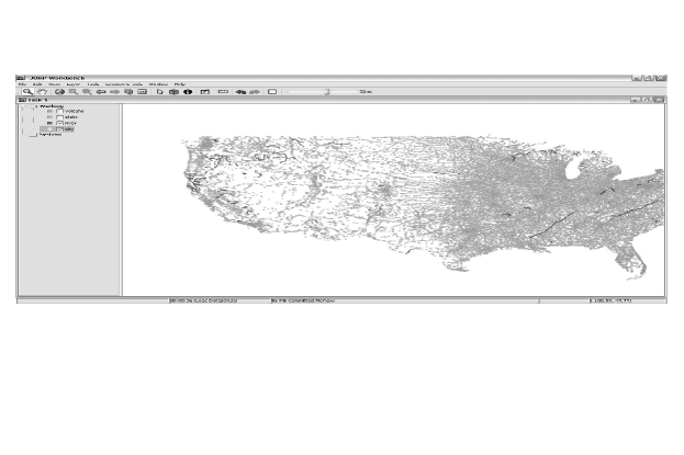
Figure 1: Running example: layer containing cities and rivers in North America.

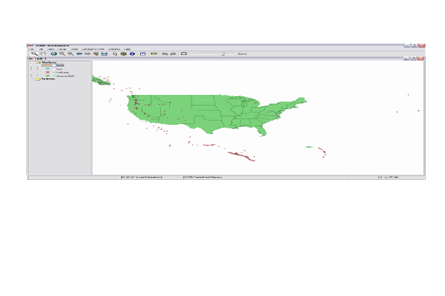
Figure 2: Running example: layer containing in states in North America and volcanoes in the northern hemisphere.

1.2 Contributions

We propose a formal model for spatial aggregation that supports efficient evaluation of aggregate queries in spatial databases based on the OLAP paradigm. This model is aimed at integrating GIS and OLAP in a unique framework. A GIS dimension is defined as a set of hierarchies of geometric elements (e.g., polygons, polylines), where the bottom level of each hierarchy, denoted the algebraic part of the dimension, is a spatial database that stores the spatial data by means of polynomial constraints [29]. An intermediate part, denoted the geometric part, stores the identifiers of the geometric elements in the GIS. Besides these components, conventional data warehousing and OLAP components are stored as usual [16, 17, 22]. A function associates the GIS and OLAP worlds. We also define the notion of geometric aggregation, that allows to express a wide range of complex aggregate queries over regions defined as semi-algebraic sets. In this way, our proposal supports aggregation of geometric components, aggregation of measures associated with those components defined in GIS fact tables, and aggregation of measures defined in data warehouses, external to the GIS system. As far as we are aware of, this is the first effort in giving a formal framework to this problem.

Although the framework described above is general enough to express many interesting and complex queries, in practice, dealing with geometries and semi-algebraic sets can be difficult and computationally expensive. Indeed, many practical problems can be solved without going into such level of detail. Thus, as our second contribution, we identify a class of queries that we denote summable. These queries can be answered without accessing the algebraic part of the dimensions. Thus, we formally define summable queries, and study when a geometric aggregate query is or is not summable.

More often than not, summable queries involve the overlapping of thematic layers. We will show in this paper that summable queries can be efficiently evaluated precomputing the common sub-polygonization of the plane (in a nutshell, a sub-division of the plane along the “carriers” of the geometric components of a set of overlayed layers), and give a conceptual framework for this process. Our ultimate idea is to provide a working alternative to standard R-tree-based query processing. A query optimizer may take advantage of the existence of a set of precomputed overlayed layers, and choose it as the better strategy for answering a given query. We introduce Piet, an implementation of our proposal (named after the Dutch painter Piet Mondrian), built usingopen source tools, along with experimental results that show that, contrary to the usual belief [7], precomputing the common sub-polygonization can successfully compete, for some GIS and aggregate spatial queries, with typical R-tree-based solutions used in most commercial GIS. The Piet software architecture is prepared to support not only overlay precomputation as a query processing method, but R-Trees, or aR-Trees [25] as well. Our implementation also provides a smooth integration between OLAP and GIS applications, in the sense that the output of a spatial query can be used for typical roll-up and drill-down navigation. In this way, we will be able to address four kinds of queries: (a) Standard GIS queries (like “branches located in states crossed by rivers”); (b) standard OLAP queries (“total number of units sold by branch and by product”); (c) Geometric aggregation queries (“total population in states with more than three airports”); (d) Integrated GIS-OLAP queries (“total sales by product in cities crossed by a river”). OLAP-style navigation is also allowed in the latter case. Queries can submitted from a graphical interface, or written in a query language denoted GISOLAP-QL. We sketch this language in Section 6. The basic idea of this language is that a query is divided into a GIS and an OLAP part. The set of geometric objects returned by the former is passed to the OLAP part, and evaluated using Mondrian, an OLAP engine, allowing further navigation in the usual OLAP style.

Finally, and as a particular application of the ideas presented in this paper, we define the notion of generic geometric aggregate queries. In particular, we discuss topological aggregation queries, and sketch how they can be efficiently evaluated by using a topological invariant instead of geometric elements.

The remainder of the paper is organized as follows. In Section 2 we provide a brief background on GIS, and review previous approaches to the interaction between GIS and OLAP. Section 3 introduces the concept of Spatial OLAP and its data model. In Section 4, we describe summable queries, while Section 5 studies overlay precomputation. Section 6 describes GIS and OLAP integration, and introduces the GISOLAP-QL query language, a simple query language used by our implementation to answer the kinds of queries described above. In Section 7 we describe the implementation of our proposal and Section 8 discusses the results of experimental evaluation. Finally, Section 9 discusses the problem of topological aggregation queries. We conclude in Section 10.

2 Background and Related Work

2.1 GIS

In general, the information in a GIS application is divided over several thematic layers. The information in each layer consists of purely spatial data on the one hand that is combined with classical alpha-numeric attribute data on the other hand (usually stored in a relational database). Two main data models are used for the representation of the spatial part of the information within one layer, the vector model and the raster model. The choice of model typically depends on the data source from which the information is imported into the GIS.

The Vector Model.

The vector model is used the most in current GIS [21]. In the vector model, infinite sets of points in space are represented as finite geometric structures, or geometries, like, for example, points, polylines and polygons. More concretely, vector data within a layer consists of a finite number of tuples of the form (geometry,attributes) where a geometry can be a point, a polyline or a polygon. There are several possible data structures to actually store these geometries [38].

The Raster Model.

In the raster model, the space is sampled into pixels or cells, each one having an associated attribute or set of attributes. Usually, these cells form a uniform grid in the plane. For each cell or pixel, the sample value of some function is computed and associated to the cell as an attribute value, e.g., a numeric value or a color. In general, information represented in the raster model is organized into zones, where the cells of a zone have the same value for some attribute(s). The raster model has very efficient indexing structures and it is very well-suited to model continuous change but its disadvantages include its size and the cost of computing the zones. Figure 3 shows an example of data represented in the raster model. It represents the elevation in some region, the intensity of the color indicates the height. So, the dark part could indicate the summit.

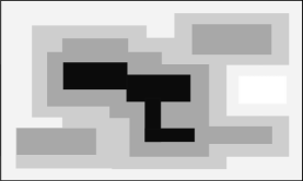
Figure 3: An example of data represented in the raster model.

The spatial information in the different thematic layers in a GIS is often joined or overlayed. Queries requiring map overlay are more difficult to compute in the vector model than in the raster model. On the other hand, the vector model offers a concise representation of the data, independent on the resolution. For a uniform treatment of different layers given in the vector or the raster model, we will, in this paper, treat the raster model as a special case of the vector model. Indeed, conceptually, each cell is, and each pixel can be regarded as, a small polygon; also, the attribute value associated to the cell or pixel can be regarded as an attribute in the vector model. This uniform approach is particularly important when we want to overlay different thematic layers on top of each other, as will become apparent in Section 5.

2.2 GIS and OLAP Interaction

Although some authors have pointed out the benefits of combining GIS and OLAP, not much work has been done in this field. Vega López et al. [37] present a comprehensive survey on spatiotemporal aggregation that includes a section on spatial aggregation. Rivest et al. [35] introduce the concept of SOLAP (standing for Spatial OLAP), and describe the desirable features and operators a SOLAP system should have. However, they do not present a formal model for this. Han et al. [8] used OLAP techniques for materializing selected spatial objects, and proposed a so-called Spatial Data Cube. This model only supports aggregation of such spatial objects. Pedersen and Tryfona [30] propose pre-aggregation of spatial facts. First, they pre-process these facts, computing their disjoint parts in order to be able to aggregate them later, given that pre-aggregation works if the spatial properties of the objects are distributive over some aggregate function. This proposal ignores the geometry, and do not address forms other than polygons. Thus, queries like “Give me the total population of cities crossed by a river” are not supported. The authors do not report experimental results. Extending this model with the ability to represent partial containment hierarchies (useful for a location-based services environment), Jensen et al. [13] proposed a multidimensional data model for mobile services, i.e., services that deliver content to users, depending on their location. Like in the previously commented proposals, this model omits considering the geometry, limiting the set of queries that can be addressed.

With a different approach, Rao et al. [33], and Zang et al. [39] combine OLAP and GIS for querying so-called spatial data warehouses, using R-trees for accessing data in fact tables. The data warehouse is then evaluated in the usual OLAP way. Thus, they take advantage of OLAP hierarchies for locating information in the R-tree which indexes the fact table. Here, although the measures are not spatial objects, they also ignore the geometric part, limiting the scope of the queries they can address. It is assumed that some fact table, containing the ids of spatial objects exists. Moreover, these objects happen to be just points, which is quite unrealistic in a GIS environment, where different types of objects appear in the different layers. Other proposals in the area of indexing spatial and spatio-temporal data warehouses [25, 26] combine indexing with pre-aggregation, resulting in a structure denoted Aggregation R-tree (aR-tree), an R-tree that annotates each MBR (Minimal Bounding Rectangle) with the value of the aggregate function for all the objects that are enclosed by it. We implemented an aR-tree for experimentation (see Section 8). This is a very efficient solution for some particular cases, specially when a query is posed over a query region whose intersection with the objects in a map must be computed on-the-fly. However, problems may appear when leaf entries partially overlap the query window. In this case, the result must be estimated, or the actual results computed using the base tables. Kuper and Scholl [21], suggested the possible contribution of constraint database techniques to GIS. Nevertheless, they did not consider spatial aggregation, nor OLAP techniques.

In summary, although the proposals above address particular problems, no one includes a formal study of the problem of integrating spatial and warehousing information in a single framework. In the first part of this paper we propose a general solution to this problem. In the second part of the paper, we address practical and implementation issues.

3 Spatial Aggregation

3.1 Conceptual Model

Our proposal is aimed at integrating, in the same conceptual model, spatial and non-spatial information in a natural way. We assume the latter to be stored in a data warehouse, following the standard OLAP notion of dimension hierarchies and fact tables [17, 1, 12]. Both kinds of information may have even been produced and stored completely separated from each other. Integrating them in the same data model would allow to support complex queries, specifically queries involving aggregation over regions defined by the user, as we will see later. We will take advantage of the fact that the vector model for spatial data (see Section 2) leads naturally to a definition of a hierarchy of geometries. For instance, points are associated with polylines, polylines with polygons, and so on, conveying a graph (actually a DAG) where the nodes are dimension levels representing geometries, and there is an edge from geometry $G_{a}$ to geometry $G_{b}$ if elements in $G_{b}$ are composed by elements in $G_{a}.$ The model allows a point in space to aggregate over more than one element of an associated geometry.

In our model, a GIS dimension is composed, as usual in databases, of a dimension schema and dimension instances. Each dimension is composed of a set of graphs, each one describing a set of geometries in a thematic layer. Figure 4 shows a GIS dimension schema (we also show a Time dimension, which we comment later), with three hierarchies, located in three different layers, following our running example: rivers ($L_{r}$), volcanoes ($L_{v}$), and states ($L_{e}$) (other layers can be represented analogously). We define three sectors, denoted the Algebraic part, the Geometric part, and the Classical OLAP part. Typically, each layer contains a set of binary relations between geometries of a single kind (although the latter is not mandatory). For example, an instance of the relationship (line,polyline) will store the ids of the lines belonging to a polyline.

There is always a finest level in the dimension schema, represented by a node with no incoming edges. We assume, without loss of generality that this level, called “point”, represents points in space. The level “point” belongs to the Algebraic part of the conceptual model. Here, data in each layer are represented as infinite sets of points $(x,y)$. We assume that the elements in the algebraic part are finitely described by means of linear algebraic equalities and inequalities. In the Geometric part, data consist of a finite number of elements of certain geometries. This part is used for solving the geometric part of a query, for instance to find all polygons that compose the shape of a country. Each point in the Algebraic part corresponds to one or more elements in the Geometric part. Note that, for example, it can be the case where a point corresponds to two adjacent polygons, or to the intersection of two or more roads. (We will see later that, during the sub-polygonization process, the plane will be divided in a set of open convex polygons, and, in that case, a point will correspond to a unique polygon, conveying a kind of functional dependency). There is also a distinguished level, denoted “All”, with no outgoing edges.

Non-spatial information is represented in the OLAP part, and is associated to levels in the geometric part. For example, information about states, stored in a relational data warehouse, can be associated to polygons, or information about rivers, to polylines. Typically, these concepts are represented as a set of dimension levels or categories, which are part of a hierarchy in the usual OLAP sense. Note that, as a general rule, we can characterize the information in the OLAP part as application-dependent.

Besides the information representing geometric components (i.e., the GIS), we also consider the existence of a Time dimension (actually, there could be more than one Time dimension, supporting, for example, different notions of time). Figure 4 shows a configuration of a Time dimension following the standard OLAP convention. Note that the OLAP part could also contain the time dimension. However, considering this dimension separately makes it easier to extend the model to address spatio-temporal data, like in [20].

Example 1

In Figure 4, the level polygon in layer $L_{e}$ is associated with two dimension levels, $state$ and $region$, such that $state\rightarrow region$ (“$A\rightarrow B$” means that there is a functional dependency from level $A$ to level $B$ in the OLAP part [1]). Each dimension level may even have attributes associated, like population, number of schools, and so on. Thus, a geometrically-represented component is associated with a dimension level in the OLAP part. There is also an OLAP hierarchy associated to the layer $L_{r}$ at the level of polyline. Notice that since dimension levels are associated to geometries, it is straightforward to associate facts stored in a data warehouse in the OLAP part, in order to aggregate these facts along geometric dimensions, as we will see later. Finally, note that in the algebraic part, the relationship represented by the edge $\langle point,polygon\rangle$ associates infinite point sets with polygons.

$\sqcap$$\sqcup$

Figure 4: An example of a GIS dimension Schema

We will now define the data model in a formal way. Let us assume the following sets: a set of layer names $\mathbf{L}$, a set $\mathbf{A}$ of attribute and dimension level names, $\mathbf{D}$ a set of OLAP dimension names, and a set $\mathbf{G}$ of geometry names. Each element $\mathrm{a}$ of $\mathbf{A}$ has an associated set of values $dom(\mathrm{a})$. We assume that $\mathbf{G}$ contains at least the following elements (geometries): point, node, line, polyline, polygon and the distinguished element “All”. More can be added. Each geometry $\mathrm{G}$ of $\mathbf{G}$ has an associated domain $dom(\mathrm{G})$. The domain of Point, $dom(\mathrm{Point})$, for example, is the set of all pairs in $\mathbb{R}^{2}$. The domain of All = $\{\mathrm{all}\}$. The domain of the elements $\mathrm{G}$ of $\mathbf{G}$, except $\mathrm{Point}$ and $\mathrm{All}$, is is a set of geometry identifiers, $\mathrm{g_{id}}.$ In other words, $\mathrm{g_{id}}$ are identifiers of geometry instances, like polylines or polygons.

Definition 1 (GIS Dimension Schema)

Given a layer $L\in\mathbf{L},$ a geometry graph $\mathrm{H}(L)=(\mathrm{N},\mathrm{E})$ is a graph defined as follows (where $\mathrm{N}$ and $\mathrm{E}$ are two unary and binary relations, respectively):

• there is a tuple $\langle\mathrm{G}\rangle$ in $\mathrm{N}$ for each kind of geometry $\mathrm{G}\in\mathbf{G}$ in $L$;

• there is a tuple $\langle\mathrm{G_{i}},\mathrm{G_{j}}\rangle$ in $E$ if $\mathrm{G_{j}}$ is composed by geometries of type $\mathrm{G_{i}}$ (i.e., the granularity of $\mathrm{G_{j}}$ is coarser than that of $\mathrm{G_{i}}$), where $\mathrm{G_{i}}$ and $\mathrm{G_{j}}\in\mathbf{G}$;

• there is a distinguished member $All$ that has no outgoing edges;

• there is exactly one tuple $\langle point\rangle$ in $\mathrm{H}(L),$ such that point is a node in the graph, that has no incoming edges;

The OLAP part is composed by a set of dimension schemas $\mathcal{D}$ defined as in [12], where each dimension $\mathrm{D}\in\mathcal{D}$ is a tuple of the form $\langle dname,\mathrm{A},\preceq\rangle,$ such that $dname$ is the dimension’s name, where $\mathrm{A}\in\mathbf{A},$ is a set of dimension levels, and $\preceq$ is a partial order between levels.

There is also a set $\mathcal{A}$ of partial functions $Att$ with signature $\mathbf{A}\times\mathbf{D}\rightarrow\mathbf{G}\times\mathbf{L}$ mapping attributes in OLAP dimensions to geometries in layers (see also Definition 2).

Finally, a GIS dimension schema is tuple $\mathrm{G}_{sch}=\langle\mathcal{H},\mathcal{A},\mathcal{D}\rangle$ where $\mathcal{H}$ is the finite set $\{\mathrm{H}_{1}(L_{1}),\ldots\mathrm{H}_{k}(L_{k})\}.$     $\sqcap$$\sqcup$

Example 2

Figure 4 depicts the following dimension schema. The geometry graph is defined by:
$\mathrm{H}_{1}(L_{r})=(\{\mathrm{point},\mathrm{line},\mathrm{polyline},\mathrm{All}\},$ $\{(\mathrm{point},\mathrm{line}),$ $(\mathrm{line},$ $\mathrm{polyline}),$ $(\mathrm{polyline},\mathrm{All})\});$
$\mathrm{H}_{2}(L_{v})=(\{\mathrm{point},\mathrm{node},\mathrm{All}\},$ $\{(\mathrm{point},\mathrm{node}),$ $(\mathrm{node},\mathrm{All})\});$
$\mathrm{H}_{3}(L_{e})=(\{\mathrm{point},\mathrm{polygon},\mathrm{All}\},$ $\{(\mathrm{point},\mathrm{polygon}),\\ (\mathrm{polygon},$ $\mathrm{All})\}).$

In the OLAP part we have dimensions Rivers and States. Then, the $Att$ functions are:
$Att(\mathrm{state},\mathrm{States})=(\mathrm{polygon},L_{e}),$ and $Att(\mathrm{river},\mathrm{Rivers})=(\mathrm{polyline},L_{r}).$ Moreover, in dimension States, it holds that $\mathrm{state}\preceq\mathrm{region}$ (we omit the schemas for the sake of brevity). Therefore, the GIS dimension schema is:
$\mathrm{G}_{sch}=\langle\{(\mathrm{H}_{1}(L_{r}),(\mathrm{H}_{2}(L_{v}),\mathrm{H}_{3}(L_{e})\},\{Att(\mathrm{state}),$ $Att(\mathrm{river})\},$ $\{Rivers,States\}\rangle.$

$\sqcap$$\sqcup$

Definition 2 (GIS Dimension Instance)

Let $\mathrm{G}_{sch}=\langle\mathcal{H},\mathcal{A},\mathcal{D}\rangle$ be a GIS dimension schema. A GIS dimension instance is a tuple $\langle\mathrm{G}_{sch},\mathcal{R},\mathcal{A}_{inst},\mathcal{D}_{inst}\rangle,$ where $\mathcal{R}$ is a set of relations $r_{L_{i}}^{\mathrm{G}_{j}\rightarrow\mathrm{G}_{k}}$ in $dom(\mathrm{G}_{j})\times dom(\mathrm{G}_{k})$, corresponding to each pair of levels such that there is an edge from $\mathrm{G}_{j}$ to $\mathrm{G}_{k}$ in the geometry graph $\mathrm{H}_{i}(L_{i})$ in $\mathrm{G}_{sch}.$ We denote each relation $r_{L_{i}}^{\mathrm{G}_{j}\rightarrow\mathrm{G}_{k}}$ in $\mathcal{R},$ a rollup relation.

Associated to each function $Att$ such that $Att(\mathrm{A,D})$ $=(\mathrm{G},\mathrm{L}),$ there is a function $\alpha_{L,D}^{\mathrm{A\rightarrow G}}\in\mathcal{A}_{inst}.$ Here, $D$ is the name of a dimension in the OLAP part. The use of this function $\alpha$ will be clear in Example 5. Intuitively, the function provides a link between a data warehouse instance and an instance of the hierarchy graph: an element in a level $A$ in a dimension $D$ in the OLAP part, is mapped to a unique instance of a geometry in the graph corresponding to a layer $L$ in the geometric part.

Finally, for each dimension schema $D\in\mathcal{D}$ there is a dimension instance defined as in [12], which is a tuple $\langle D,RUP\rangle,$ where $RUP$ is a set of rollup functions that relate elements in the different dimension levels (intuitively, these rollup functions indicate how the attribute values in the OLAP part are aggregated).

$\sqcap$$\sqcup$

Example 3

Figure 5 shows a portion of a GIS dimension instance for the layer $L_{r}$ in the dimension schema of Figure 4. In this example, we can see that an instance of a GIS dimension in the OLAP part is associated to the polyline $pl_{1},$ which corresponds to the Colorado river. For simplicity we only show four different points at the $point$ level $\{(x_{1},y_{1}),\ldots,(x_{4},y_{4})\}.$ There is a relation $r_{L_{r}}^{point\rightarrow line}$ containing the association of points to the lines in the line level. Analogously, there is also a relation $r_{L_{r}}^{line\rightarrow polyline},$ between the line and polyline levels, in the same layer.     $\sqcap$$\sqcup$

Figure 5: A portion of a GIS dimension instance in Figure 4.

Elements in the geometric part in Definition 1 can be associated with facts, each fact being quantified by one or more measures, not necessarily a numeric value.

Definition 3 (GIS Fact Table)

Given a Geometry $\mathrm{G}$ in a geometry graph $\mathrm{H}(L)$ of a GIS dimension schema $\mathrm{G}_{sch}$ and a list $\mathrm{M}$ of measures $(M_{1},\ldots,M_{k}),$ a GIS Fact Table schema is a tuple $FT=(\mathrm{G},\mathrm{L},\mathrm{M})$. A tuple $BFT=({\mathrm{p}oint},\mathrm{L},\mathrm{M})$ is denoted a Base GIS Fact Table schema. A GIS Fact Table instance is a function $ft$ that maps values in $dom(G)\times\mathrm{L}$ to values in $dom(\mathrm{M_{1}})\times\cdots\times dom(\mathrm{M_{k}}).$ A Base GIS Fact Table instance maps values in $\mathbb{R}^{2}\times\mathrm{L}$ to values in $dom(\mathrm{M_{1}})\times\cdots\times dom(\mathrm{M_{k}}).$

$\sqcap$$\sqcup$

Besides the GIS fact tables, there may also be classical fact tables in the OLAP part, defined in terms of the OLAP dimension schemas. For instance, instead of storing the population associated to a polygon identifier, as in Example 4, the same information may reside in a data warehouse, with schema $(state,year,population).$

Example 4

Consider a fact table containing state populations in our running example. Also assume that this information will be stored at the polygon level. In this case, the fact table schema would be $(polyId,L_{e},population),$ where Population is the measure. If information about, for example, temperature data, is stored at the point level, we would have a base fact table with schema $(point,$ $L_{e},temperature),$ with instances like $(x_{1},y_{1},L_{e},25).$ Note that temporal information could be also stored in these fact tables, by simply adding the Time dimension to the fact table. This would allow to store temperature information across time.     $\sqcap$$\sqcup$

3.2 Geometric Aggregation

In Section 1 we gave the intuition of spatial aggregate queries. We now formally define this concept, and denote it geometric aggregation.

Definition 4 (Geometric Aggregation)

Given a GIS dimension as introduced in Definitions 1 and 2, a Geometric Aggregation is an expression of the form

$$\int\!\!\int_{\mathbb{R}^{2}}~{}\delta_{C}(x,y)~{}h(x,y)~{}dx\,dy,$$

where $C=\{(x,y)\in\mathbb{R}^{2}\mid\varphi(x,y)\},$ and $\delta_{C}$ is defined as follows:

$\delta_{C}(x,y)=1$ on the two-dimensional parts of $C;$ it is a Dirac delta function [4] on the zero-dimensional parts of $C;$ and it is the product of a Dirac delta function with a combination of Heaviside step functions [11] for the one-dimensional parts of $C$ (see Remark 2 below for details). Here, $\varphi$ is a FO-formula in a multi-sorted logic $\mathcal{L}$ over $\mathbb{R}$, $\mathbf{L}$ and $\mathbf{A}$. The vocabulary of ${\cal L}$ contains the function names appearing in $\mathcal{F}$ and $\mathcal{A}$, together with the binary functions $+$ and $\times$ on real numbers, the binary predicate $<$ on real numbers and the real constants $0$ and $1$. Further, also constants for layers and attributes may appear in $\cal L$. Atomic formulas in ${\cal L}$ are combined with the standard logical operators $\land$, $\vee$ and $\neg$ and existential and universal quantifiers over real variables and attribute variables. Furthermore, $h$ is an integrable function constructed from elements of $\{1,ft\}$ using arithmetic operations.     $\sqcap$$\sqcup$

Remark 1

The sets $C$ in Definition 4 are known in mathematics as semi-algebraic sets. In the GIS practice, only linear sets (points, polylines and polygons) are used. Therefore, it could suffice to work with addition over the reals only, leaving out multiplication.     $\sqcap$$\sqcup$

Remark 2

A simple example of a one-dimensional Dirac delta function [4] (or impulse function) $\delta_{a}(x)$ for a real number $a$ can be $\lim_{\varepsilon\rightarrow\infty}f_{a}(\varepsilon,x),$ where $f_{a}(\varepsilon,x)=$ $\varepsilon$ if $a-\frac{1}{2\varepsilon}\leq x\leq a+\frac{1}{2\varepsilon}$ and $f_{a}(\varepsilon,x)=0$ elsewhere. For a two-dimensional point $(a,b)$ in $\mathbb{R}^{2}$, we can define the two-dimensional Dirac delta function $\delta_{(a,b)}(x,y)$ as $\lim_{\varepsilon\rightarrow\infty}f_{(a,b)}(\varepsilon,x,y)$, with $f_{(a,b)}(\varepsilon,x,y)=\varepsilon^{2}$ if $a-\frac{1}{2\varepsilon}\leq x\leq a+\frac{1}{2\varepsilon}$ and $b-\frac{1}{2\varepsilon}\leq y\leq b+\frac{1}{2\varepsilon}$ and $f_{(a,b)}(\varepsilon,x,y)=0$ elsewhere.

If $C$ is a finite set of points in the plane, then the delta function of $C$, $\delta_{C}(x,y)$, is defined as $\sum_{(a,b)\in C}\delta_{(a,b)}(x,y)$. It has the property that $\int\!\!\!\int_{\mathbb{R}^{2}}\delta_{C}(x,y)\,dxdy$ is equal to the cardinality of $C$. Intuitively, including a Dirac delta function in geometric aggregation, allows to express geometric aggregate queries like “number of airports in a region $C$”.

If $C$ is a one-dimensional curve, then the definition of $\delta_{C}(x,y)$ is more complicated. Perpendicular to $C$ we can use a one-dimensional Dirac delta function, and along $C$, we multiply it with a combination of Heaviside step functions [11]. The one-dimensional Heaviside step function is defined as $H(x)=1$ if $x\geq 0$ and $H(x)=0$ if $x<0$. For $C$, we can define a Heaviside function $H_{C}(x,y)=1$ if $(x,y)\in C$ and $H_{C}(x,y)=0$ outside $C$. As a simple example, let us consider the curve $C$ given by the equation $y=0$ $\land$ $0\leq x\leq L$. The function $\delta_{C}(x,y)$, in this case, can be defined as $\delta_{0}(y)\cdot H(x)\cdot H(L-x)$. The one-dimensional Dirac delta function $\delta_{0}(y)$ takes care of the fact that perpendicular to $C$, an impulse is created. The factors $H(x)$ and $H(L-x)$ take care of the fact that this impulse is limited to $C$. In this case, it is easy to see that $\int\!\!\!\int_{\mathbb{R}^{2}}\delta_{C}(x,y)\,dxdy$ is the length of $C$ and in fact this is true for arbitrary $C$. For arbitrary $C$, the definition of $\delta_{C}$ is rather complicated and involves the use of $H_{C}(x,y)$. We omit the details. Intuitively, this combination of functions allows to express geometric aggregate queries like “Give me the length of the Colorado river”.

Remark 3

The expression given by Definition 4 is the basic construct for geometric aggregation queries. More complicated queries can be written as combinations of this basic construct by means of arithmetic operators. For example, a query asking for the total number of airports per square kilometer would require dividing the geometric aggregation that computes the number of airports in the query region, by the geometric aggregation computing the area of such region.

The framework presented so far, allows to express complex queries that take into account geometric features, data associated to these features, and data stored externally, probably in a data warehouse. Example 5 shows a series of geometric aggregate queries.

Example 5

The following queries refer to our running example, introduced in Section 1. The thematic layers containing information about cities and rivers are labeled $L_{c}$ and $L_{r},$ respectively. In order to make the queries more interesting, we defined cities as polygons instead of the point representation shown in Figure 1. For simplicity, we will denote $\mathrm{H_{L_{c}}}$ the hierarchy graph $\mathrm{H}(L_{c}).$ The hierarchy graphs $\mathrm{H_{L_{c}}}$ and $\mathrm{H_{L_{r}}}$ are, respectively: $\mathrm{H}_{L_{c}}=(\{\mathrm{point},\mathrm{polygon},\mathrm{All}\},\{(\mathrm{point},\mathrm{polygon}),(\mathrm{polygon},\mathrm{All})\}),$ $\mathrm{H}_{L_{r}}=(\{\mathrm{point},\mathrm{line},\mathrm{polyline},\mathrm{All}\},\{(\mathrm{point},\mathrm{line}),(\mathrm{line},\newline \mathrm{polyline}),(\mathrm{polyline},\mathrm{All})\})$. The population density for each coordinate in $L_{c}$ is stored in a base fact table $ft_{pop}$ (we assume it is stored in some finite way, i.e., using polynomial equations over the real numbers, as in Example 4). Furthermore, we have $Att(\mathrm{city},\mathrm{Cities})=(\mathrm{polygon},\mathrm{L_{c}}),$ and $Att(\mathrm{river},\mathrm{Rivers})=(\mathrm{polyline},\mathrm{L_{r}}).$ In what follows, we will abbreviate $\mathrm{Point}$, $\mathrm{Polygon}$ and $\mathrm{PolyLine}$ by $\mathrm{Pt}$, $\mathrm{Pg}$ and $\mathrm{Pl}$ respectively. Also, $\mathrm{Ci}$ and $\mathrm{Ri}$ will stand for the attributes $\mathrm{city}$ and $\mathrm{river},$ respectively. Finally, note that in the queries below, the Dirac delta function is such that $\delta_{C}(x,y)=1,$ inside the region $C,$ and $\delta_{C}(x,y)=0,$ outside this region.

• Q₁: Total population of all cities within 100km from San Francisco.

  $$Q_{\mathrm{1}}\equiv\int\!\!\int_{C_{1}}~{}ft_{pop}(x,y,L_{c})dx\,dy,$$

  where $C_{1}$ is defined by the expression:

  $$\halign{\hbox to\displaywidth{$\hfil\displaystyle#\hfil$}\cr 0.0pt{\hfil$\displaystyle\qquad C_{1}=\{(x,y)\in\mathbb{R}^{2}~{}|~{}(\exists x^{\prime})(~{}\exists y^{\prime})(\exists x^{\prime\prime})(~{}\exists y^{\prime\prime})(~{}\exists pg_{1})\cr 0.0pt{\hfil$\displaystyle(~{}\exists pg_{2})(\exists c\in dom(Ci))\hfill{}\cr 0.0pt{\hfil$\displaystyle\hfill{}(\alpha_{L_{c},Cities}^{\mathrm{Ci}\rightarrow\mathrm{Pg}}(\mbox{`San Francisco'})=pg_{1}~{}\land~{}r_{L_{c}}^{\mathrm{Pt}\rightarrow\mathrm{Pg}}(x^{\prime},y^{\prime},pg_{1})~{}\land\hfill{}\cr 0.0pt{\hfil$\displaystyle\hfill{}\alpha_{L_{c},Cities}^{\mathrm{Ci}\rightarrow\mathrm{Pg}}(c)=pg_{2}~{}\land~{}r_{L_{c}}^{\mathrm{Pt}\rightarrow\mathrm{Pg}}(x^{\prime\prime},y^{\prime\prime},pg_{2})~{}\land~{}pg_{2}\neq pg_{1}~{}\land\hfill{}\cr 0.0pt{\hfil$\displaystyle\hfill{}((x^{\prime\prime}-x^{\prime})^{2}+(y^{\prime\prime}-y^{\prime})^{2}\leq 100^{2})~{}\land\hfill{}\cr 0.0pt{\hfil$\displaystyle\hfill{}r_{L_{c}}^{\mathrm{Pt}\rightarrow\mathrm{Pg}}(x,y,pg_{2}))\}.\qquad\crcr}}}}}}}$$

  The meaning of the query is the following: function $\alpha_{L_{c},Cities}^{\mathrm{Ci}\rightarrow\mathrm{Pg}}$ maps a city in dimension Cities to a polygon in layer $L_{c}$ (representing cities). Thus, the third line in the expression for $C_{1}$ maps San Francisco to a polygon in that layer. The fourth and fifth lines find the cities within 100 Km of San Francisco. The sixth line shows the relation $r_{L_{c}}^{\mathrm{Pt}\rightarrow\mathrm{Pg}}$ with the mapping between the points and the polygons representing the cities that satisfy the condition.

• Q₂: Total population of the cities crossed by the Colorado river.

  $$Q_{\mathrm{2}}\equiv\int\!\!\int_{C_{2}}~{}ft_{pop}(x,y,L_{c})~{}dx\,dy,\mathrm{\/where}$$

  $$\halign{\hbox to\displaywidth{$\hfil\displaystyle#\hfil$}\cr 0.0pt{\hfil$\displaystyle\qquad C_{2}=\{(x,y)\in\mathbb{R}^{2}~{}|~{}(\exists x^{\prime})(~{}\exists y^{\prime})(~{}\exists pl_{1})(~{}\exists pg_{1})\cr 0.0pt{\hfil$\displaystyle(\exists c\in dom(Ci))\hfill{}\cr 0.0pt{\hfil$\displaystyle\hfill{}(\alpha_{L_{r},Rivers}^{\mathrm{Ri}\rightarrow\mathrm{Pl}}(\mbox{`Colorado'})=pl_{1}~{}\land~{}r_{L_{r}}^{\mathrm{Pt}\rightarrow\mathrm{Pl}}(x^{\prime},y^{\prime},pl_{1})~{}\land\hfill{}\cr 0.0pt{\hfil$\displaystyle\hfill{}\alpha_{L_{c},Cities}^{\mathrm{Ci}\rightarrow\mathrm{Pg}}(c)=pg_{1}~{}\land~{}r_{L_{c}}^{\mathrm{Pt}\rightarrow\mathrm{Pg}}(x^{\prime},y^{\prime},pg_{1})~{}\land\hfill{}\cr 0.0pt{\hfil$\displaystyle\hfill{}r_{L_{c}}^{\mathrm{Pt}\rightarrow\mathrm{Pg}}(x,y,pg_{1}))\}.\qquad\crcr}}}}}}$$

• Q₃: Total population endangered by a poisonous cloud described by $\varphi,$ a formula in first-order logic over $(\mathbb{R},+,\allowbreak\times,\allowbreak<,\allowbreak 0,1)$).

  $$Q_{\mathrm{3}}\equiv\int\!\!\int_{C_{3}}~{}ft_{pop}(x,y,L_{c})dx\,dy,$$

  $$\mathrm{\/where\/}~{}C_{3}=\{(x,y)\in\mathbb{R}^{2}~{}|~{}\varphi(x,y)\}.$$

$\sqcap$$\sqcup$

4 Summable Queries

The framework we presented in previous sections is general enough to allow expressing complex geometric aggregation queries (Definition 4) over a GIS in an elegant way. However, computing these queries within this framework can be extremely costly, as the following discussion will show.

Let us consider again Example 5. Here $ft_{pop}$ is a density function. This could be a constant function over cities, e.g., the density in all points of San Francisco, say, $1000$ people per square kilometer. But $ft_{pop}$ is allowed to be more complex too, like for instance a piecewise constant density function or even a very precise function describing the true density at any point. Moreover, just computing the expression “$C$” of Definition 4 could be practically infeasible. In Example 5, query Q${}_{\mathrm{2}},$ computing on-the-fly the intersection (overlay) of the cities and rivers is likely to be very expensive, as would be, in query Q₃ of the same example, computing the algebraic formula $\varphi.$

In this section we will identify a subclass of geometric aggregate queries that facilitates computing the integral over $h(x,y)$, as defined in Definition 4. As a result, query evaluation becomes more efficient than for geometric aggregation queries in general. In the next section we will see how we can also get rid of the algebraic part for computing the region “C”.

We first look for a way of avoiding the computation of the integral of the functions $h(x,y)$ of Definition 4. Specifically, we will show that storing less precise information (for instance, having a simpler function $ft_{pop}$ in Example 5) results in a more efficient computation of the integral. There are queries, like Q₃ of Example 5, were even if the function $ft_{pop}$ is piecewise constant over the cities, there is no other way of computing the population over the region defined by $\varphi$ than taking the integral, as $\varphi$ can define any semi-algebraic set. Further, just computing the population within an arbitrarily given region cannot be performed. However, for queries Q₁ and Q₂ the situation is different. Indeed, the sets $C_{1}$ and $C_{2}$ return a finite set of polygons, representing cities. If the function $ft_{pop}$ is constant for each city, it suffices to compute $ft_{pop}$ once for each polygon, and then multiply this value with the area of the polygon. Summing up the products would yield the correct result, without the need of integrating $ft_{pop}$ over the area $C_{1}$ or $C_{2}.$ This is exactly the subclass of queries we want to propose, those that can be rewritten as sums of functions of geometric objects returned by condition “$C$”. We will denote these queries summable.

Definition 5 (Summable Query)

A geometric aggregation query $Q=$
$\int\int_{\mathbb{R}^{2}}~{}\delta_{C}(x,y)~{}h(x,y)~{}dx\,dy$ is summable if and only if:

1. $C=\bigcup_{g\in G}ext(g),$ where $G$ is a set of geometric objects, and $ext(g)$ means the geometric extension of $g.$

2. There exists $h^{\prime},$ constructed using $\{1,f_{t}\}$ and arithmetic operators, such that

   $$Q=\sum_{g\in S}h^{\prime}(g),$$

   with $h^{\prime}(g)=\int\int_{\mathbb{R}^{2}}\delta_{ext(g)}(x,y)~{}h(x,y)~{}dx\,dy.$

$\sqcap$$\sqcup$

Working with less accurate functions for this type of queries means that the Base GIS fact tables should not be mappings from $\mathbb{R}^{2}\times\mathbf{L}$ to measures, but from $dom(\mathrm{G})\times\mathbf{L}$ to measures, for those $\mathrm{g}$ in $r_{L}^{\mathrm{point}\rightarrow\mathrm{G}}$.

Example 6

Let us reconsider the queries Q₁ and Q₂ from Example 5. The function $ft_{pop}$ now maps elements of $dom(\mathrm{Polygon})$ to populations. Observe that the sets $C^{\prime}_{1}$ and $C^{\prime}_{2}$ return a finite set of polygons, indicated by their id’s (denoted $g_{id}$).

• Q₁: Total population of all cities within 100km from San Francisco. Now, the set $C^{\prime}_{1}$ is defined in terms of the points in the algebraic part, and the identifiers of the polygons satisfying the constraint.

  $$Q_{\mathrm{1}}\equiv\sum_{\mathrm{g_{id}}\in C^{\prime}_{1}}~{}ft_{pop}(\mathrm{g_{id}},L_{c}).$$

  $$\halign{\hbox to\displaywidth{$\hfil\displaystyle#\hfil$}\cr 0.0pt{\hfil$\displaystyle\qquad C^{\prime}_{1}=\{g_{id}~{}|~{}(\exists x)(~{}\exists y)(\exists x^{\prime})(~{}\exists y^{\prime})(\exists pg_{1})\cr 0.0pt{\hfil$\displaystyle(\exists c\in dom(Ci))\hfill{}\cr 0.0pt{\hfil$\displaystyle\hfill{}(\alpha_{L_{c},Cities}^{\mathrm{Ci}\rightarrow\mathrm{Pg}}(\mbox{`San Francisco'})=pg_{1}~{}\land~{}r_{L_{c}}^{\mathrm{Pt}\rightarrow\mathrm{Pg}}(x,y,pg_{1})~{}\land\hfill{}\cr 0.0pt{\hfil$\displaystyle\hfill{}\alpha_{L_{c},Cities}^{\mathrm{Ci}\rightarrow\mathrm{Pg}}(c)=g_{id}~{}\land r_{L_{c}}^{\mathrm{Pt}\rightarrow\mathrm{Pg}}(x^{\prime},y^{\prime},g_{id})~{}\land~{}pg_{1}\neq g_{id}~{}\land\hfill{}\cr 0.0pt{\hfil$\displaystyle\hfill{}((x^{\prime}-x)^{2}+(y^{\prime}-y)^{2}\leq 100^{2})\qquad\crcr}}}}}}$$

• Q₂: Total population of the cities crossed by the Colorado river.

  $$Q_{\mathrm{2}}\equiv\sum_{\mathrm{g_{id}}\in C^{\prime}_{2}}~{}ft_{pop}(\mathrm{g_{id}},L_{c}).$$

  $$\halign{\hbox to\displaywidth{$\hfil\displaystyle#\hfil$}\cr 0.0pt{\hfil$\displaystyle\qquad C^{\prime}_{2}=\{g_{id}~{}|~{}(\exists x)(~{}\exists y)(~{}\exists pl_{1})(\exists c\in dom(Ci))\hfill{}\cr 0.0pt{\hfil$\displaystyle\hfill{}(\alpha_{L_{r},Rivers}^{\mathrm{Ri}\rightarrow\mathrm{Pl}}(\mbox{`Colorado'})=pl_{1}~{}\land~{}r_{L_{r}}^{\mathrm{Pt}\rightarrow\mathrm{Pl}}(x,y,pl_{1})~{}\land\hfill{}\cr 0.0pt{\hfil$\displaystyle\hfill{}\alpha_{L_{c},Cities}^{\mathrm{Ci},\rightarrow\mathrm{Pg}}(c)=g_{id}\land r_{L_{c}}^{\mathrm{Pt}\rightarrow\mathrm{Pg}}(x,y,g_{id}))\}.\qquad\crcr}}}}$$

$\sqcap$$\sqcup$

Queries aggregating over zero or one-dimensional regions (like, for instance, queries requiring counting the number of occurrences of some phenomena) can also be summable, as the next examples show.

Example 7

Let us denote $L_{a}$ a layer containing airports in our running example. We would like to count the number of airports in some region. Also, remember that $\alpha_{L_{c},Cities}^{\mathrm{Ci}\rightarrow\mathrm{Pg}}$ maps cities in a dimension Cities to polygon identifiers in a layer $L_{c}$ (i.e., Ci are sets of cities and Pg are sets of polygons).

• Q₄: Number of airports located in San Francisco. This is expressed by:

  $$Q_{\mathrm{4}}\equiv\sum_{\mathrm{g_{id}}\in C^{\prime}_{4}}1,$$

  where $C^{\prime}_{4}$ is defined by the expression:

  $$\halign{\hbox to\displaywidth{$\hfil\displaystyle#\hfil$}\cr 0.0pt{\hfil$\displaystyle\qquad C^{\prime}_{4}=\{g_{id}~{}|~{}(\exists x)(~{}\exists y)(\exists pg_{1})\hfill{}\cr 0.0pt{\hfil$\displaystyle\hfill{}(\alpha_{L_{c},Cities}^{\mathrm{Ci}\rightarrow\mathrm{Pg}}(\mbox{`San Francisco'})=pg_{1}~{}\land~{}r_{L_{c}}^{\mathrm{Pt}\rightarrow\mathrm{Pg}}(x,y,pg_{1})~{}\land\hfill{}\cr 0.0pt{\hfil$\displaystyle\hfill{}r_{L_{a}}^{\mathrm{Pt}\rightarrow\mathrm{Node}}(x,y,g_{id}))\}.\qquad\crcr}}}}$$

  Here, San Francisco, in the OLAP part, is mapped to a polygon $pg_{1},$ through the $\alpha_{L_{c},Cities}^{\mathrm{Ci}\rightarrow\mathrm{Pg}}$ function. The relation $r_{L_{a}}^{\mathrm{Pt}\rightarrow\mathrm{Node}}(x,y,g_{id})$ links points to nodes representing airports in the $L_{a}$ layer (in this case, this relation actually represents a mapping from points to nodes).

  Analogously, but with a more complex condition, query Q₅ below shows a sum over a set of identifiers that correspond to cities crossed by rivers.

• Q₅: How many cities are crossed by the Colorado river?

  $$Q_{\mathrm{5}}\equiv\sum_{\mathrm{g_{id}}\in C^{\prime}_{5}}~{}1.$$

  $$\halign{\hbox to\displaywidth{$\hfil\displaystyle#\hfil$}\cr 0.0pt{\hfil$\displaystyle\qquad C^{\prime}_{5}=\{g_{id}~{}|~{}(\exists x)(~{}\exists y)(~{}\exists pl_{1})(\exists c\in dom(Ci))\hfill{}\cr 0.0pt{\hfil$\displaystyle\hfill{}(\alpha_{L_{r},Rivers}^{\mathrm{Ri}\rightarrow\mathrm{Pl}}(\mbox{`Colorado'})=pl_{1}~{}\land~{}r_{L_{r}}^{\mathrm{Pt}\rightarrow\mathrm{Pl}}(x,y,pl_{1})\land\hfill{}\cr 0.0pt{\hfil$\displaystyle\hfill{}\alpha_{L_{c},Cities}^{\mathrm{Ci}\rightarrow\mathrm{Pg}}(\mbox{c})=g_{id}~{}\land~{}r_{L_{c}}^{\mathrm{Pt}\rightarrow\mathrm{Pg}}(x,y,g_{id})\qquad\crcr}}}}$$

  The last example query shows that the aggregation can also be expressed over a fact table in the application part of the model.

• Q₆: How many students are there in cities crossed by the Colorado river?

  $$Q_{\mathrm{6}}\equiv\sum_{\mathrm{Ci}\in C^{\prime}_{6}}~{}ft_{cities}^{\#students}(\rm Ci).$$

  $$\halign{\hbox to\displaywidth{$\hfil\displaystyle#\hfil$}\cr 0.0pt{\hfil$\displaystyle\qquad C^{\prime}_{6}=\{c\in dom(C_{i})~{}|~{}(\exists x)(~{}\exists y)(~{}\exists pg_{1})(~{}\exists pl_{1})\hfill{}\cr 0.0pt{\hfil$\displaystyle\hfill{}\alpha_{L_{r},Rivers}^{\mathrm{Ri}\rightarrow\mathrm{Pl}}(\mbox{`Colorado'})=pl_{1}~{}\land~{}r_{L_{r}}^{\mathrm{Pt}\rightarrow\mathrm{Pl}}(x,y,pl_{1})\land\hfill{}\cr 0.0pt{\hfil$\displaystyle\hfill{}\alpha_{L_{c},Cities}^{\mathrm{Ci}\rightarrow\mathrm{Pg}}(\mbox{c})=pg_{1}~{}\land~{}r_{L_{c}}^{\mathrm{Pt}\rightarrow\mathrm{Pg}}(x,y,pg_{1}))\}.\qquad\crcr}}}}$$

$\sqcap$$\sqcup$

Query $Q_{\mathrm{6}}$ shows that the sum is performed over a set of city identifiers (this would be “C”, the integration region), and a function that maps cities to the number of students in them. The latter could be a fact table containing the city identifiers and, as a measure, the number of students (for type consistency we assume that $ft_{cities}^{\#students}$ is a projection of the fact table over the measure of interest). This fact table is outside the geometry of the GIS. Note, then, that summable queries integrate GIS and OLAP worlds in an elegant way.

Summable queries are useful in practice because, most of the time, we do not have information about parts of an object, like, for instance, the population of a part of a city. On the contrary, populations are often given by totals per city or province, etc. In this case, we may divide the city, for example, in a set of sub-polygons such that each sub-polygon represents a neighborhood. Thus, queries asking for information on such neighborhoods become summable.

Algorithm 1 below, decides if $C$ is of the form $\bigcup_{g\in G}ext(g).$ If $C$ is of this form, then the second condition of Definition 5 is automatically satisfied.

Algorithm 1

boolean DecideSummability$(C)$
Input: A query region “C”.
Output: “True”, if “C” is a finite set of elements of a geometry representing the query region for $Q.$ “False” otherwise.

1.  for each layer $L$ and each geometry $G$ in $L$  do

2.     $S=\phi;$

3.     for each $g\in G$ do

4.        if $ext(g)\subseteq C$ then

5.           $S=S\cup\{g\};$

6.     if $C=\bigcup_{g\in S}ext(g)$  then

7.        Return “True”;

8.     Return “False”.

Once we have established that $C$ is a finite union of elements $g$ of some geometry $G$, it is easy to see how $h^{\prime}$ can be obtained from $h$. Indeed, for each $g\in G$, we can define $h^{\prime}(g)$ as $\int\!\!\int_{\mathbb{R}^{2}}~{}\delta_{ext(g)}(x,y)~{}h(x,y)~{}dx\,dy$. Since $h$ is built from the constant 1, fact table values and arithmetic operations, also $h^{\prime}$ can be seen to be constructible from 1, fact table values (at the level of summarization of the elements of $G$) and arithmetic operations.

The above decision algorithm can easily be turned into an algorithm that produces, for a given “C”, an equivalent description as a union of elements of some geometry. Once this description is found it is straightforward to find the function $h^{\prime}.$ This is illustrated by the aggregate queries $Q_{\mathrm{1}}$ and $Q_{\mathrm{2}}$ that are given in both forms in Sections 3 and 4 respectively.

5 Overlay Precomputation

Many interesting queries in GIS boil down to computing intersections, unions, etc., of objects that are in different layers. Hereto, their overlay has to be computed. In Section 4 we have shown many examples of such queries. Queries $Q_{\mathrm{2}},$ $Q_{\mathrm{5}},$ and $Q_{\mathrm{6}}$ are typical examples where cities crossed by rivers have to be returned. The on-the-fly computation of the sets “C” containing all those cities, is costly because most of the time we need to go down to the Algebraic part of the system, and compute the intersection between the geometries (e.g., states and rivers, cities and airports, and so on). Therefore, we will study the possibilities and consequences of precomputing the overlay operation and show that this can be an efficient alternative for evaluating queries of this kind. R-trees [6], and aR-trees  [25, 26] can also be used to efficiently compute these intersections on-the-fly. In Section 8 we discuss this issue, and compare indexing and overlay pre-computation.

We need some definitions in order to explain how we are going to compute the overlay of different thematic layers.

We will work within a bounding box $\mathrm{B}\times\mathrm{B}$ in $\mathbb{R}^{2},$ where $\mathrm{B}$ is a closed interval of $\mathbb{R}$, as it is usual in GIS practice. We showed in Section 1 that in practice we will consider the bounding box as an additional layer. Also, in what follows, a line segment is given as a pair of points, and a polyline as a tuple of points.

Definition 6 (The carrier set of a layer)

The carrier set $C_{\mathrm{pl}}$ of a polyline $\mathrm{pl}=(p_{0},p_{1},\ldots,p_{(l-1)},p_{l})$ consists of all lines that share infinitely many points with the polyline, together with the two lines through $p_{0}$ and $p_{l},$ and perpendicular to the segments $(p_{0},p_{1})$ and $(p_{(l-1)},p_{l})$, respectively. Analogously, the carrier set $C_{\mathrm{pg}}$ of a polygon $\mathrm{pg}$ is the set of all lines that share infinitely many points with the boundary of the polygon. Finally, the carrier set $C_{\mathrm{p}}$ of a point $\mathrm{p}$ consists of the horizontal and the vertical lines intersecting in the point. The carrier set $C_{\mathrm{L}}$ of a layer $\mathrm{L}$ is the union of the carrier sets of the points, polylines and polygons appearing in the layer. Figure 6 illustrates the carrier sets of a point, a polyline and a polygon.     $\sqcap$$\sqcup$

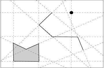
Figure 6: The carrier sets of a point, a polyline and a polygon are the dotted lines.

The carrier set of a layer induces a partition of the plane into open convex polygons, open line segments and points.

Definition 7

Let $C_{\mathrm{L}}$ be the carrier set of a layer $\mathrm{L}$, and let $\mathrm{B}\times\mathrm{B}$ in $\mathbb{R}^{2}$ be a bounding box. The set of open convex polygons, open line segments and points, induced by $C_{\mathrm{L}}$, that are strictly inside the bounding box, is called the convex polygonization of $\mathrm{L}$, denoted $CP(\mathrm{L})$.     $\sqcap$$\sqcup$

5.1 Sub-polygonization of multiple layers

In former sections we have explained that usual GIS applications represent information in different thematic layers. For instance, cities (represented a polygons or points, depending on the adopted scale) may be described in a layer, while rivers (polylines) can be stored in another one. In our proposal, these thematic layers will be overlayed by means of the common sub-polygonization operation, that further subdivides the bounding box $\mathrm{B}\times\mathrm{B}$ according to the carrier sets of the layers involved.

Definition 8 (Sub-polygonization)

Given two layers $\mathrm{L}_{1}$ and $\mathrm{L}_{2},$ and their carrier sets $C_{\mathrm{L}_{1}}$ and $C_{\mathrm{L}_{2}},$ the common sub-polygonization of $\mathrm{L}_{1}$ according to $\mathrm{L}_{2}$, denoted $\mathrm{CSP}({\mathrm{L}_{1}},{\mathrm{L}_{2}})$ is a refinement of the convex polygonization of $\mathrm{L}_{1}$, computed by partitioning each open convex polygon and each open line segment in it along the carriers of $C_{\mathrm{L}_{2}}$.     $\sqcap$$\sqcup$

Definition 8 can be generalized for more than two layers, denoted $\mathrm{CSP}({\mathrm{L}_{1}},{\mathrm{L}_{2}},\ldots,{\mathrm{L}_{k}}).$ It can be shown that the overlay-operation on planar subdivision induced by a set of carriers is commutative and associative. The proof is straightforward, and we omit it for the sake of space.

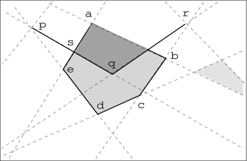
Figure 7: The common sub-polygonization of a layer.

Example 8

Figure 7 shows the common sub-polygonization of a layer $L_{c}$ containing one city (the pentagon with corner points $a$, $b$, $c$, $d$ and $e$), and another layer, $L_{r}$, containing one river (the polyline $pqr$). The open line segment $]s,q[$ belongs to both $L_{c}$ and $L_{r}$, as it is part of both the river and the city. The open polygons in the partition of the city (e.g., the dark shaded open quadrangle) belong only to $L_{c}$, and the light shaded open polygon on the right hand side of Figure 7 belongs to no layer whatsoever.     $\sqcap$$\sqcup$

The question that naturally arises is: why do we use the carriers of geometric objects in the computation of the overlay operation, instead of just the points and line segments that bound those objects?. There are several reasons for this. First, consider the situation in the left frame of Figure 8. A river $rqp$ originates somewhere in a city, and then leaves it. The standard map overlay operation divides the river in two parts: one part, $rq$, inside the city, and the other one, $qp$, outside the city. Nevertheless, the city layer is not affected. On the one hand, we cannot leave the city unaffected, as our goal is in fact to pre-compute the overlay. On the other hand, partitioning the city into the line segment $rq$ and the polygon $abcd$ without the line segment $rq$ results in an object which is not a polygon anymore. Such a shape is not only very unnatural, but, for example, computing its area may cause difficulties. With the common sub-polygonization we have guaranteed convex polygons. Many useful operations on polygons become very simple if the polygons are convex (e.g., triangulation, computing the area, etc.). A second reason for the common sub-poligonization is that it gives more precise information. The right frame of Figure 8 shows the polygonization of the left frame. The partition of the city into more parts, also dependent on where the river originates, allows us to query, for instance, parts of the city with fertile and dry soil, depending on the presence of the river in those parts. As a more concrete example, let us suppose the following query:

Q₇: Total length of the part of the Colorado river that flows through the state of Nevada. The following expression may solve the problem.

$$Q_{\mathrm{7}}\equiv\sum_{\mathrm{g_{id}}\in C^{\prime}_{7}}~{}ft_{length}(\mathrm{g_{id}},L_{r}),$$

where $C^{\prime}_{7}$ is the set:

$$\halign{\hbox to\displaywidth{$\hfil\displaystyle#\hfil$}\cr 0.0pt{\hfil$\displaystyle\qquad C^{\prime}_{7}=\{g_{id}~{}|~{}(\exists x)(~{}\exists y)\hfill{}\cr 0.0pt{\hfil$\displaystyle\hfill{}(\alpha_{L_{r},Rivers}^{\mathrm{Ri}\rightarrow\mathrm{Pl}}(\mbox{`Colorado'})=g_{1}~{}\land~{}r_{L_{r}}^{\mathrm{Pt}\rightarrow\mathrm{Pl}}(x,y,g_{1})\land\hfill{}\cr 0.0pt{\hfil$\displaystyle\hfill{}\alpha_{L_{e},States}^{\mathrm{St}\rightarrow\mathrm{Pg}}(\mbox{`Nevada'})=g_{2}~{}\land~{}r_{L_{e}}^{\mathrm{Pt}\rightarrow\mathrm{Pg}}(x,y,g_{2})\land\hfill{}\cr 0.0pt{\hfil$\displaystyle\hfill{}r_{L_{r}}^{\mathrm{Pt}\rightarrow\mathrm{Li}}(x,y,g_{id})\land r_{L_{r}}^{\mathrm{Li}\rightarrow\mathrm{Pl}}(g_{id},g_{1}))\qquad\crcr}}}}}$$

Note that in our running example, the function $Att$ in layer $L_{r}$ (i.e., representing rivers) maps values to elements at the polyline level. However, we must return the identifiers of the lines that corresponds to the polyline that represents the Colorado river. Relation $r_{L_{r}}^{\mathrm{Li}\rightarrow\mathrm{Pl}}(g_{id},g_{1})$ is used to compute such identifiers. Note that the expression above gives the correct answer to Query Q₇ when the river is such that the polyline representing it lies within the state boundaries (for instance, it would not work if the river is represented as polyline with a straight line passing through Nevada). When this is not the case, a common sub-polygonization would solve the problem.

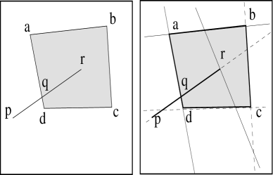
Figure 8: Common sub-polygonization vs. map overlay.

5.1.1 Using the common sub-polygonization

From a conceptual point of view, we characterize the common sub-polygonization of a set of layers as a schema transformation of the GIS dimensions involved. Basically, this operation reduces to update hierarchy graphs of Definition 1. For this, we base ourselves on the notion of dimension updates introduced by Hurtado et al. [12], who also provide efficient algorithms for such updates. Dimension updates allow, for instance, inserting a new level into a dimension and its corresponding rollup functions or splitting/merging dimension levels. The difference here is that in the original graph we have relations instead of rollup functions.

Consider the hierarchy graphs $\mathrm{H}_{1}(L_{1})$ and ${H}_{2}(L_{2})$ depicted on the left hand side of Figure 9. After computing the common sub-polygonization, the hierarchy graph is updated as follows: there is a unique hierarchy (remember that $\mathrm{CSP}({\mathrm{L}_{1}},{\mathrm{L}_{2}})=\mathrm{CSP}({\mathrm{L}_{2}},{\mathrm{L}_{1}})$) with bottom level Point, and three levels of the type Node (a geometry containing single points in $\mathbb{R}^{2}$), OPolyline (which stands for open polyline, or polyline without end points) and OPolygon (which stands for open polygon, i.e., a polygon without its bordering polyline). Also, level Polyline is inserted between levels OPolyline and Polygon. These levels are added by means of update operators analogous to the ones described in [12]. We will not explain this procedure here, we limit ourselves to show the final result. Note that now we have all the geometries in a common layer (in the example below we show the impact of this fact). The right hand side of Figure 9 shows the updated dimension graph. We remark that, for clarity we have merged the two layers into a single one, although we may have kept both layers separately. Finally, at the instance level the rollup functions are updated accordingly. For instance, each polyline in a layer is partitioned into the set of points and open line segments belonging to the sub-polygonization that are part of that polyline. A consequence of the subdivision in open polygons and polylines is that now, instead of the relations $r_{L_{i}}^{\mathrm{G}_{j}\rightarrow\mathrm{G}_{k}}$ we will have functions, which we will call rollup functions, denoted $f_{L}^{\mathrm{G}_{j}\rightarrow\mathrm{G}_{k}}$. Thus, taking, for example layer $\mathrm{L}_{1}$, the relation $r_{\mathrm{L}_{1}}^{\mathrm{Pt}\rightarrow\mathrm{Pl}}$ will be replaced by the functions $f_{\mathrm{L}}^{\mathrm{Pt}\rightarrow\mathrm{Node}}$, $f_{\mathrm{L}}^{\mathrm{Pt}\rightarrow\mathrm{OPl}}$ and $f_{\mathrm{L}}^{\mathrm{Pt}\rightarrow\mathrm{OPg}}$.

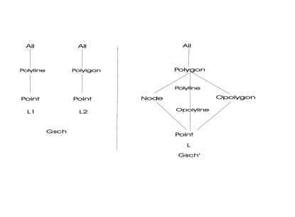
Figure 9: Updated dimension schema.

We investigate the effects of the common sub-polygoni- zation over the evaluation of summable queries. Specifically, we propose (a) to evaluate summable queries using the common sub-polygonization; and (b) to precompute the common sub-polygonization. Precomputation is a well-known technique in query evaluation, particularly in the OLAP setting. As in common practice, the user can choose to precompute all possible overlays, or only the combinations most likely to be required. The implementation we show in the next section supports both policies.

Let us consider again query Q₂ from Example 5 (“Total population of cities crossed by the Colorado river”). Recall that the summable version of the query reads:

$$\mathrm{Q}_{\mathrm{2}}\equiv\sum_{\mathrm{g_{id}}\in C^{\prime}_{2}}~{}ft_{pop}(\mathrm{g_{id},L_{c}}).$$

In Example 5 we have expressed the region $C^{\prime}_{2}$ in terms of the elements of the algebraic part of the GIS schema. However, the common sub-polygonization, along with its precomputation, allows us to get rid of this part, and only refer to the ids of the geometries involved, also for computing the query region. In this way, the set $C^{\prime}_{2},$ will be expressed in terms of open polygons ($\mathrm{OPg}$), open polylines ($\mathrm{OPl}$) and points. Hence, $C^{\prime}_{2}$ now reads:

$$\halign{\hbox to\displaywidth{$\hfil\displaystyle#\hfil$}\cr 0.0pt{\hfil$\displaystyle\qquad C^{\prime}_{2}=\{g_{id}\in G_{id}\mid(\exists g_{id}^{\prime}\in G_{id})(\exists c\in dom(Ci))\hfill{}\cr 0.0pt{\hfil$\displaystyle\hfill{}(f_{L}^{\mathrm{OPl}\rightarrow\mathrm{Pg}}(g_{id}^{\prime})=g_{id}\hfill{}\cr 0.0pt{\hfil$\displaystyle\hfill{}~{}\land~{}\alpha_{L,Cities}^{\mathrm{Ci}\rightarrow\mathrm{OPg}}(c)=g_{id}\hfill{}\cr 0.0pt{\hfil$\displaystyle\hfill{}\land\ \alpha_{L,Rivers}^{\mathrm{Ri}\rightarrow\mathrm{OPl}}(\mbox{`Colorado'})=g_{id}^{\prime})\}.\qquad\crcr}}}}}$$

Note that the expression for $C^{\prime}_{2}$ uses the rollup functions of the updated GIS dimensions, and only deals with object identifiers. Also, $L$ represents the common sub-polygonization layer. Therefore, computing $C^{\prime}_{2}$ reduces to looking for objects with a certain identifier. Also, we got rid of the layer subscripts, because now we are working with a unique layer.

Now, we can see that query Q₇ (“Total length of the part of the Colorado river that flows through the state of Nevada”) can be computed in a precise way. The query region will be, for this case:

$$\halign{\hbox to\displaywidth{$\hfil\displaystyle#\hfil$}\cr 0.0pt{\hfil$\displaystyle\qquad C^{\prime}_{7}=\{g_{id}\in G_{id}~{}|~{}\hfill{}\cr 0.0pt{\hfil$\displaystyle\hfill{}(\alpha_{L,Rivers}^{\mathrm{Ri}\rightarrow\mathrm{Pl}}(\mbox{`Colorado'})=f_{L}^{\mathrm{OPl}\rightarrow\mathrm{Pl}}(g_{id})~{}\land\hfill{}\cr 0.0pt{\hfil$\displaystyle\hfill{}\alpha_{L,States}^{\mathrm{St}\rightarrow\mathrm{Pg}}(\mbox{`Nevada'})=f_{L}^{\mathrm{OPl}\rightarrow\mathrm{Pg}}(g_{id})~{}\land\hfill{}\cr 0.0pt{\hfil$\displaystyle\hfill{}f_{L}^{\mathrm{Pt}\rightarrow\mathrm{OPl}}(g^{\prime}_{id}))=g_{id})\}.\qquad\crcr}}}}}$$

In Section 7 we explain the sub-polygonization process in detail.

5.1.2 Complexity

Let $G_{Sch}$ be the GIS dimension schema on the left-hand side of Figure 9. Let $G_{Inst}$ be an instance containing a set of polygons $R$, a set of points $P$ and a set of polylines $L$. Moreover, let the maximum number of corner points of a polygon and the maximum number of line segments composing a polyline be denoted $n_{R}$ and $n_{L},$ respectively. The carrier set of all layers, i.e., the union of the carrier sets for each layer separately, (see Definition 6) then contains at most $N=2|P|+|L|(n_{L}+2)+|R|n_{R}$ elements. These carriers represent a so-called planar subdivision, i.e., a partition of the plane into points, open line segments and open polygons. Planar subdivisions are studied in computational geometry [3]. It is a well-known fact that the complexity of a planar subdivision induced by $N$ carriers is $O(N^{2})$.

Property 1 (Complexity of planar subdivision)

Given a planar subdivision induced by $N$ carriers:

(i) The number of points is at most $\frac{N(N-1)}{2}$;

(ii) The number of open line segments is at most $N^{2}$;

(iii) The number of open convex polygons is at most $\frac{N^{2}}{2}+\frac{N}{2}+1$.     $\sqcap$$\sqcup$

The complexity of the planar subdivision is defined as the sum of the three expressions in Property 1.

It follows that, if we precompute the overlay operation, in the worst case, the instance $G^{\prime}_{Inst}$ of the updated schema $G^{\prime}_{Sch}$ becomes quadratic in the size of the original instance $G_{Inst}$. However, as different layers typically store different types of information, the intersection will be only a small part of $G^{\prime}_{Inst}$. Moreover, several elements of $G^{\prime}_{Inst}$ will not be of interest to any layer (see Example 8), and can be discarded.

6 GIS-OLAP Integration

The framework introduced in Section 3 allows a seamless integration between the GIS and OLAP worlds. From a query language point of view, GIS-OLAP integration allows combining, in a single expression, queries about geometric and OLAP content (e.g., total sales in branches in states crossed by rivers in the last four years), without losing the ability to express standard GIS or OLAP queries.

In our proposal, denoted Piet (after Piet Mondrian, the painter whose name was adopted for the open source OLAP system we also use in the implementation), GIS and OLAP integration is achieved through two mechanisms: (a) a metadata model, denoted Piet Schema; and (b) a query language, denoted GISOLAP-QL, where a query is composed of two sections: a GIS section, denoted GIS-Query, with a specific syntax, and an OLAP section, OLAP-Query, with MDX syntax .

6.1 Piet-Schema

Piet-Schema is a set of metadata definitions,. These include: the storage location of the geometric components and their associated measures, the subgeometries corresponding to the sub-polygonization of all the layers in a map, and the relationships between the geometric components and the OLAP information used to answer integrated GIS and OLAP queries. Piet uses this information to answer the queries written in the language we describe in Section 6.2. Metadata are stored in XML documents containing three kinds of elements: Subpoligonization, Layer, and Measure. An example of a Subpoligonization element is shown below:

<Subpolygonization>
     <SubPLevel name="Polygon"
      table="gis_subp_polygon_4"
      primaryKey="id" uniqueIdColumn="uniqueid"
      originalGeometryColumn="originalgeometryid"/>
     <SubPLevel name="Linestring"
      table="gis_subp_linestring_4"
      primaryKey="id" uniqueIdColumn="uniqueid"
      originalGeometryColumn="originalgeometryid"/>
     <SubPLevel name="Point" table="gis_subp_point_4"
      primaryKey="id" uniqueIdColumn="uniqueid"
      originalGeometryColumn="originalgeometryid"/>
</Subpolygonization>

The element includes the location of each subgeometry (subnode, subpolygon or subline) in the data repository (in our implementation, the PostGIS database where the map is stored). It also has the name of the table containing each subgeometry, the names of the key fields, and the identifiers allowing to associate geometries and subgeometries.

Below we show an element layer that describes information of each of the layers that compose a map, and their relationship with the subgeometries and the data warehouse. The Piet-Schema contains a list with a layer element for each layer in a map.

<Layer name="usa_states" hasAll="true"
 table="usa_states"
 primaryKey="id" geometry="geometry"
 descriptionField="name">
    <Properties>
        <Property name="Population" column="f_pop"
         type="Double" />
        <Property name="Total income" column="f_a13"
         type="Double" />
        <Property name="Total number of jobs"
         column="f_a34" type="Double" />
        <Property name="Male pop" column="f_male"
         type="Double" />
        <Property name="Female Pop" column="f_female"
         type="Double" />
        <Property name="Under 18 Pop"
         column="f_under18" type="Double" />
        <Property name="Middle Age Pop"
         column="f_medage" type="Double" />
        <Property name="Over 65 Pop"
         column="f_perover65"  type="Double" />
    </Properties>
    <SubpolygonizationLevels>
        <SubPUsedLevel name="Polygon" />
        <SubPUsedLevel name="Linestring" />
        <SubPUsedLevel name="Point" />
    </SubpolygonizationLevels>
    <OLAPRelation table="gis_olap_states"
    gisId="gisid"
    olapId="olapid" olapDimensionName="Store"
    olapLevelName="Store State">
        <OlapTable name="store" id="state_id"
        hierarchyNameField="store_state"
        hierarchyAll="[Store].[All Stores]" />
    </OLAPRelation>
</Layer>

The element layer contains the name of the layer, the name of the table storing the actual data, the name of the key fields, the geometry and the description. The list Properties details the facts associated to geometric components of the layer, including name, field name, and data type. Element SubpolygonizationLevel indicates the sub-polygonization levels that can be used (for instance, if it is a layer representing rivers, only point and line could be used). Finally, the relationship (if it exists) between the layer and the data warehouse is defined in the element OLAPRelation, that includes the identifiers of the geometry and the associated OLAP object, and the hierarchy level this object belongs to. An element OLAPTable also includes the MDX statement used to insert a new dimension in the original GISOLAP-QL expression. In the portion of the XML document depicted above, the association between the states in the map and the states in the data warehouse is performed through the table gis_olap_states (using the attribute state_id). Figure 10 shows some columns and rows of the table Stores in the data warehouse, associated to this XML document.

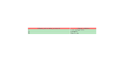
Figure 10: Portion of the table Stores in the data warehouse for our running example.

The last component of Piet-Schema definition contains a list of measure elements where the measures associated to geometric components in the GIS dimension are specified.

<Measure name = "StoresQuantity" layer="usa_stores"
aggregator="count"/> <Measure name = "RiverSegments"
layer="usa_rivers" aggregator="count"/>

6.2 The GISOLAP-QL Query Language

GISOLAP-QL has a very simple syntax, allowing to express integrated GIS and OLAP queries. For the OLAP part of the query we kept the syntax and semantics of MDX. A GISOLAP-QL query is of the form:

GIS-Query $|$ OLAP-Query

A pipe (“$|$”) separates two query sections: a GIS query and an OLAP query. The OLAP section of the query applies to the OLAP part of the data model (namely, the data warehouse) and is written in MDX. The GIS part of the query has the typical SELECT FROM WHERE SQL form, except for a separator (“;”) at the end of each clause:

SELECT list of layers and/or measures;

FROM Piet-Schema;

WHERE geometric operations;

The SELECT clause is composed of a list of layers and/or measures, which must be defined in the corresponding Piet-Schema of the FROM clause. The query returns the geometric components (or their associated measures) that belong to the layers in the SELECT clause, and verify the conditions in the WHERE clause.

The FROM clause just contains the name of the schema used in the query. The WHERE clause in the GIS-Query part, consists in conjunctions and/or disjunctions of geometric operations applied over all the elements of the layers involved. The expression also includes the kind of subgeometry used to perform the operation (this is only used if the sub-polygonization technique is selected to solve the query). The syntax for an operation is:

operation name(list of layer members, subgeometry)

Although any typical geometric operation can be supported, our current implementation supports the “intersection” and “contains” operations. The accepted values for subgeometry are “Point”, “LineString” and “Polygon” . For example, the following expression computes the states which contain at least one river, using the subgeometries of type linestring generated and associated during the overlay precomputation.

Contains(layer.usa_states,layer.usa_rivers,subplevel.Linestring)

The WHERE clause can also mention a query region (the region where the query must be evaluated).

Example 9

The query “description of rivers, cities and store branches, for branches in cites crossed by a river” reads:

SELECT layer.usa_rivers, layer.usa_cities, layer.usa_stores;

FROM Piet-Schema;

WHERE intersection(layer.usa_rivers,

layer.usa_cities,subplevel.Linestring)

and contains(layer.usa_cities,

layer.usa_stores,subplevel.Point);

The query returns the components $r,$ $s,$ and $c$ in the layers usa_rivers, usa_stores and usa_cities respectively, such that $r$ and $c$ intersect, and $s$ is contained in $c$ (i.e., the coordinates of the point that represents $s$ in layer usa_stores are included in the region determined by the polygon that represents $c$ in layer usa_cities). The result is shown in Figure 11. In other words, if $L$ is a list of attributes (geometric components) in the SELECT clause, $I=\{(r_{1},c_{1}),$ $(r_{2},c_{2}),$ $(r_{3},c_{3})\}$ is the result of the intersection operation, and $C=\{(c_{1},s_{1}),$ $(c_{2},s_{2})\}$ is the result of the contains operation, the semantics of the query above is given, operationally, by $\rm\Pi_{L}(I\Join C).$

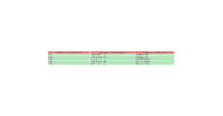
Figure 11: Query result for “rivers, cities and store branches, for the branches in cities crossed by a river”.

The query “number of branches by city” uses a geometric measure defined in Piet-Schema. The query reads (the result is shown in Figure 12):

SELECT layer.usa_cities,measure.StoresQuantity;

FROM Piet-Schema;

WHERE intersection(layer.usa_cities,

layer.usa_stores,subplevel.Point);

Figure 12: Query result for branches per city.

GISOLAP-QL queries that select particular dimension members are also supported. For example, the following query returns the airports, cities and branches for the state with id=6 (result shown in Figure 13):

SELECT layer.usa_cities,layer.usa_airports,layer.usa_stores;

FROM Piet-Schema;

WHERE intersection(usa_states.6,layer.usa_cities,

subplevel.Point) and

intersection(usa_states.6,layer.usa_airports,

subplevel.Point) and

intersection(usa_states.6,layer.usa_stores,

subplevel.Point);
    $\sqcap$$\sqcup$

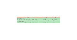
Figure 13: Query result for airports, cities and stores in state with id=6.

6.3 Spatial OLAP with GISOLAP-QL

A user who needs to perform OLAP operations that involve a data warehouse associated to geographic components, will write a “full” GISOLAP-QL query, i.e., a query composed of the GIS and OLAP parts. The latter is simply an MDX query, that receive as input the result returned by the GIS portion of the query. Consider for instance the query: “total number of units sold and their cost, by product, promotion media (v.g., radio, TV, newspapers) and state”. The GISOLAP-QL expression will read:

SELECT layer.usa_states;

FROM Piet-Schema;

WHERE intersection(layer.usa_states, layer.usa_stores,subplevel.point);

$|$

select [Measures].[Unit Sales], [Measures].[Store Cost],

[Measures].[Store Sales]

ON columns,

$\{$([Promotion Media].[All Media], [Product].[All Products])$\}$

ON rows

from [Sales]

where [Time].[1997]

The GIS-Query returns the states which intersect store branches at the point level. The OLAP section of the query uses the measures in the data warehouse in the OLAP part of the data model (Unit Sales, Store Cost, Store Sales), in order to return the requested information. The dimensions are Promotion Media and Product. Assume that the following hierarchy defines the Store dimension: store $\rightarrow$ city $\rightarrow$ state $\rightarrow$ country $\rightarrow$ All. This hierarchy is defined in the Piet schema. In this example, let us suppose, for simplicity, that the GIS part of the query (the one in the left hand side of the GISOLAP-QL expression) returns three identifiers, 1, 2, and 3, corresponding, respectively, to the states of California, Oregon and Washington. These identifiers correspond to three ids in the OLAP part of the model, stored in a Piet mapping table.

The next step is the construction of an MDX sub-expression for each state, traversing the different dimension levels (starting from All down to state). The information is obtained from the OLAPTable XML element in Piet-Schema. Finally, the MDX clause Children is added, allowing to obtain the children of each state (in this case, the cities). For instance, one of these clauses looks like:

[Store].[All Stores].[USA].[CA].Children

The sub-expressions for the three states in this query are related using the Union and Hierarchize MDX clauses . The final MDX generated from the spatial information is:

Hierarchize( Union(Union($\{$[Store].[All Stores].

[USA].[CA].Children$\},$

$\{$[Store].[All Stores].[USA].[OR].Children)$\},$

$\{$[Store].[All Stores].[USA].[WA].Children$\}$)))

The MDX subexpression is finally added to the OLAP-query part of the original GISOLAP-QL statement. In our example, the resulting expression is:

select $\{$[Measures].[Unit Sales],

[Measures].[Store Cost],[Measures].[Store Sales]$\}$

ON columns,

Crossjoin(Hierarchize(Union(Union

($\{$[Store].[All Stores].[USA].[CA].Children$\}$,

$\{$[Store].[All Stores].[USA].[OR].Children$\}$),

$\{$[Store].[All Stores].[USA].[WA].Children$\}$)),

$\{$([Promotion Media].[All Media],

[Product].[All Products])$\}$)

ON rows

from [Sales]

where [Time].[1997]

Our Piet implementation allows the resulting MDX statement to be executed over a Mondrian engine (see Section 7 for details) in a single framework. Figure 14 shows the result for our example. The result includes the three dimensions: Store (obtained through the geometric query), Promotion Media, and Product. A Piet user can navigate this result (drilling-down or rolling-up along the dimensions). Figure 15 shows an example, drilling down starting from Seattle.

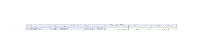
Figure 14: Query result for the full GISOLAP-QL example query.

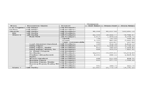
Figure 15: Drilling down starting from the result of Figure 14.

7 Implementation

In this section we describe our implementation. We first present the software architecture and components, and then we discuss the algorithmic solutions for two key aspects of the problem: accuracy and scalability.

The general system architecture is depicted in Figure 16. A Data Administrator defines the data warehouse schema, loads the GIS (maps) and OLAP (facts and hierarchies) information into a data repository, and creates a relation between both worlds (maps and facts). She also defines the information to be included in each layer. The repository is implemented over a PostgreSQL database [32]. PostgreSQL was chosen because, besides being a reliable open source database, is easy to extend and supports most of the SQL standard. GIS data is stored and managed using PostGIS [31]. PostGIS adds support for geographic objects to the PostgreSQL database. In addition, PostGIS implements all of the Open Geospatial Consortium (OGC) [24] specification except some “hard” spatial operations (the system was developed with the requirement of being OpenGIS-compliant). It is believed that PostGIS will be an important building block for all future open source spatial projects.

Figure 16: The Piet Architecture

A graphic interface is used for loading GIS and OLAP information into the system and defining the relations between both kinds of data. The GIS part of this component is based on JUMP [15], an open source software for drawing maps and exporting them to standard formats. Facts and dimension information are loaded using a customized interface. For managing OLAP data, Piet uses Mondrian [23], an open source OLAP server written in Java. We extended Mondrian in order to allow processing queries involving geometric components. The OLAP navigation tool was developed using Jpivot [14].

A Data Manager processes data in basically two ways: (a) performs GIS and OLAP data association; (b) precomputes the overlay of a set of geographic layers, adapts the affected GIS dimensions, and stores the information in the database. The Data Manager was implemented using the Java GIS Toolkit [5]. The query processor delivers a query to the module solving one of the four kinds of queries supported by our implementation, but of course, new kinds of queries (e.g., the topological queries explained in Section 9) can be easily added. Below, we explain the implementation in detail.

7.1 Piet Components

Our Piet implementation consists of two main modules: (a) Piet-JUMP, which includes (among other utilities) a graphic interface for drawing and displaying maps, and a back-end allowing overlay precomputation via the common sub-polygonization and geometric queries; (b) Piet-Web, which allows executing GISOLAP-QL and pure OLAP queries. The result of these queries can be navigated in standard OLAP fashion (performing typical roll-up and drill-down, and drill-accross operations).

Piet-JUMP Module. This module handles spatial information. It is based on the JUMP platform, which offers basic facilities for drawing maps and working with geometries. The Piet-JUMP module is made up of a series of “plug-ins” added to the JUMP platform: the Precalculate Overlay, Function Execution, GIS-OLAP association, and OLAP query plug-ins.

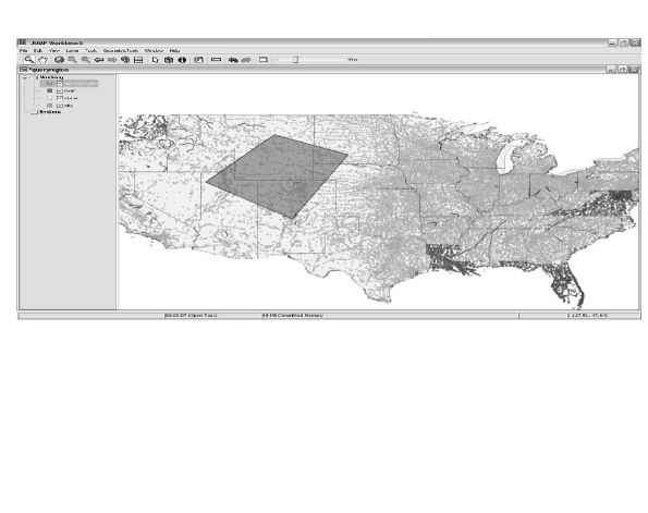
Figure 17: Defining a query region in Piet.

The Precalculate Overlay plug-in computes the overlay of a set of selected thematic layers. The information generated is used by the other plug-ins. Besides the set of layers to overlay, the user must create a layer containing only the “bounding box”. For all possible combinations of the selected layers, the plugin performs the following tasks:

(a) Generates the carrier sets of the geometries in the layers. This process creates, for each possible combination, a table containing the generated carrier lines.

(b) Computes the common sub-polygonization of the layer combination. In this step, the new geometry levels are obtained, namely: nodes, open polylines, and open polygons. This information is stored in a different table for each geometry, and each element is assigned a unique identifier.

(c) Associates the original geometries to the newly generated ones. This is the most computationally expensive process. The JTS Topology Suite was extended and improved (see below) for this task. The information obtained is stored in the database (in one table for each level, for each layer combination) in the form $<$id of an element of the sub-polygonization, id of the original geometry$>$ pairs.

(d) Propagates the values of the density functions to the geometries of the sub-polygonization. This is performed in parallel with the association process explained above.

Finally, for each combination of layers, we find all the elements in the sub-polygonization that are common to more than one geometry. In the database, a table is generated for each layer combination, and for each geometry level in the sub-polygonization (i.e., node, open line, open polygon). Each table contains the unique identifiers of each geometry, and the unique identifier of the sub-polygonization geometry common to the overlapping geometries.

The Function Execution plug-in computes a density function defined in a thematic layer, within a query region (or the entire bounding box if the query region is not defined). The user’s input are: (a) the set of layers; (b) the layer containing the query region; (c) the layer over which the function will be applied; (d) the name of the function. The result is a new layer with the geometries of the sub-polygonization and the corresponding function values. Figure 17 shows how a query region is defined in Piet. Along with the selected region, a density function is also defined. The left hand side of the screen shows the layers that could be overlayed. The graphic in the main panel shows the selected layers. Two kinds of sub-polygonizations could be used: full sub-polygonization (corresponding to the combination of all the layers) or partial sub-polygonization (involving only a subset of the layers). In the second case the process will run faster, but precision may be unacceptable, depending on how well the polygons fit the query region.

The GIS-OLAP association plug-in associates spatial information to information in a data warehouse. This information is used by the “OLAP query” plugin and the Piet-Web module. A table contains the unique identifier of the geometry, the unique identifier of the element in the data warehouse, and, optionally, a description of such element.

The OLAP query plug-in joins the two modules that compose the implementation. Starting from a spatial query and an OLAP model, the plugin generates and executes an MDX query. From this result, the user can navigate the information in the data warehouse using standard OLAP tools. The user inputs are: (a) layer with the query region; (b) layer where the geometries to associate with OLAP data are; (c) MDX query with only data warehouse information. The program associates spatial and OLAP information, and generates a new MDX query that merges both kinds of data. This query is then passed on to an OLAP tool.

Piet-Web Module. This module handles GISOLAP-QL queries, spatial aggregation queries, and even pure OLAP queries. In all cases, the result is a dataset that can be navigated using any OLAP tool. This module includes: (a) the GISOLAP-QL parser; (b) a translator to SQL; (c) a module for merging spatial and MDX queries through query re-writing, as explained in Section 6.

7.2 Robustness and Scalability Issues

As with all numerical computation using finite-precision numbers, the geometric algorithms included in Piet may present problems of robustness, i.e., incorrect results due to round-off errors. Many basic operations in the JTS library used in the Piet implementation have not yet been optimized and tuned . We extended and improved this library, and developed a new library called Piet-Utils.

Additionally, the sub-polygonization of the overlayed thematic layers generates a huge number of new geometric elements. In this setting, scalability issues must be addressed, in order to guarantee performance in practical real-world situations. Thus, we propose a partition of the map using a grid, which optimizes the computation of the sub-polygonization while preserving its geometric properties.

The two issues introduced above are addressed in this section.

7.2.1 Robustness

We will address separately the computation of the carrier lines and the sub-polygonization process.

Computation of Carrier Lines

In a Piet environment, geometries are internally represented using the vector model, with objects of type geometry included in the JTS library. Examples of instances of these objects are: POINT (378 145), LINESTRING (191 300, 280 319, 350 272, 367 300), and POLYGON (83 215, 298 213, 204 74, 120 113, 83 215). Each geometric component includes the name and a list of vertices, as pairs of (X,Y) coordinates.

The first step of the computation of the sub-polygonization is the generation of a list containing the carrier lines produced by the carrier sets of the geometric components of each layer. The original JTS functions may produce duplicated carrier lines, arising from the incorrect overlay of (apparently) similar geometric objects. For instance, if a river in one layer coincides with a state boundary in another layer, duplicated carrier lines may appear due to mathematical errors, and propagate to the polygonization step. The algorithm used in the Piet implementation eliminates these duplicated carrier lines after the carrier set is generated.

We also address the problem of minimizing the mathematical errors that may appear in the computation of the intersection between carrier lines in different layers. First, given a set of carrier lines $L_{1}$, $L_{2}$,$\ldots,$ $L_{n},$ the intersection between them is computed one line at a time, picking a line $L_{i},i=1,n-1,$ and computing its intersection with $L_{i+j},j\geq 1.$ Thus, the intersection between two lines $L_{k},L_{s}$ is always computed only once. However, it is still possible that three or more lines intersect in points very close to each other. In this case, we use a boolean function called isSimilarPoint, which, given two points and an error bound (set by the user), decides if the points are or are not the same (if the points are different they will generate new polygons). There is also a function addCutPoint which receives a point $p$ and a list $P$ of points associated to a carrier line $L.$ This function is used while computing the intersection of $L$ with the rest of the carrier lines. If there is a point in $P$, “similar” to $p,$ then $p$ is not added to $P$ (i.e., no new cut point is generated). The points are stored sorted according to their distance to the origin, in order to speed-up the similarity search. To clarify these concepts, we sketch the functions described above.

Algorithm 2

boolean isSimilarPoint$(Point~{}p1,Point~{}p2,real~{}\texttt{error})$

1.  Return result =

2.  $((-1.0)*\texttt{error}<p1.getX()-p2.getX()$ &&$p1.getX()-p2.getX()<\texttt{error}$ &&$(-1.0)*\texttt{error}<p1.getY()-p2.getY()$ &&$p1.getY()-p2.getY()<\texttt{error})$

Algorithm 3

List AddCutPoint$(Point~{}p,List~{}pointList)$

1.  if notInList(p, pointList) then

2.     position = whereToAddOrderedPoints(p, pointList)

3.     AddPointToList(p, pointList, position);

4.  Return pointList

Where notInList returns True if there is no point in pointList similar to $p$.

Example 10

Consider three carrier lines: $L_{1},$ $L_{2}$ and $L_{3}.$ $P_{1}$ is the point where $L_{1}$ intersects $L_{2}$ and $L_{3}$. Also assume that the algorithm that generates the sub-nodes is currently using $L_{2}$ as pivot line (i.e., $L_{1}$ was already used, and $L_{3}$ is still waiting). The algorithm computes the intersection between $L_{2}$ and $L_{3},$ which happens to be a point $P_{3}$ very close to $P_{1}.$ If the difference is less than a given threshold, $P_{3}$ will not be added to the list of cutpoints for $L_{2}.$ The same will happen for $L_{3}.$     $\sqcap$$\sqcup$

sub-polygonization

The points where the carrier sets intersect each other generate new geometries, denoted sub-lines. The sub-polygons are computed from the sub-lines obtained in this way, and the information is stored in the postGIS database. The sub-polygons are produced using a JTS class called Polygonizer. The enhancements to the JTS library described above ensures that no duplicated sub-lines will be used to generate the sub-polygons. As another improvement implemented in Piet for computing the sub-polygonization, the sub-lines that the Polygonizer receives do not include the lines generated by the bounding box.

The most costly process is the association of the sub-geometries to the original geometries. For this computation we also devised some techniques to improve the functions provided by the JTS library. For instance, due to mathematical errors, two adjacent sub-polygons may appear as overlapping geometries. As a consequence, the JTS intersection function provided by JTS would, erroneously, return True. We replaced this function with a new one, a boolean function denoted OverlappingPolygons (again, “error” is defined by the user.):

Algorithm 4

boolean OverlappingPolygons$(Geometry~{}p1,Geometry~{}p2,real~{}\texttt{error})$

1.  double overlappingArea = getOverlappingArea(p1, p2)

2.  Return (overlappingArea $>$ error)

7.2.2 Scalability

The sub-polygonization process is a huge CPU and (mainly), memory consumer. Even though Property 1 shows that the planar subdivision is quadratic in the worst case, for large maps, the number of sub-geometries produced may be unacceptable for some hardware architectures. This becomes worse for a high number of layers involved in the sub-polygonization. In order to address this issue, we do not compute the common sub-polygonization over an entire map. Instead, we further divide the map into a grid, and compute separately the sub-polygonization within each square in the grid. This scheme produces sub-polygons only where they are needed. It also takes advantage of the fact that, in general, the density of geometric objects in a layer is not homogeneous. In Figure 2 we can see that the density of the volcanoes is higher in the western region, and decreases toward the east. A more detailed view is provided by Figure 18, which shows a grid subdivision where a large number of empty squares. Computing the sub-polygonization due to volcanoes in these regions would be expensive and useless. It makes no sense that a carrier line generated by a volcano in the west partitions a region in the east. It seems more natural that the influence of a carrier line remains within the region of influence of the geometry that generates it. The grid subdivision solves the problem, using the notion of object of interest introduced at the end of Section 5.1.2. Reducing the number of geometric objects generated by the sub-polygonization, of course, also reduces the size of the final database containing all these “materialized views”. Also note that the squares in the grid could be of different sizes. In addition, it would be possible to compute the polygonization of the squares in the grid in parallel, provided the necessary hardware is available. As a remark, note that the grid partition also allows the refinement of a particular rectangle in the grid, if, for instance, there is an overloaded rectangle. Last but not least, the grid is also used to optimize the evaluation of a query when a query region is defined. In this case, the intersection between the sub-polygonization and the query region is computed on-the-fly. Thus, we only compute the intersection for the affected rectangles, obtaining an important improvement in the performance of these kinds of queries.

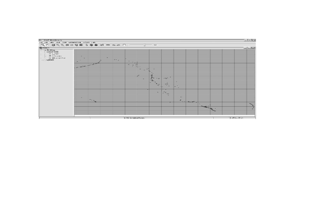
Figure 18: Running example: overlayed layers containing the grid subdivision and the volcanoes in the northern hemisphere.

8 Experimental Evaluation

We discuss the results of a set of tests, aimed at providing evidence that the overlay precomputation method, for certain classes of geometric queries (with or without aggregation) can outperform other well-established methods like R-tree indexing. In addition, we implemented the aggregation R-tree (aR-tree) [25], an R-tree which which stores, for each minimum bounding rectangle (MBR), the value of the aggregation function for all the objects enclosed by the MBR. The main goal of these tests is to determine under which conditions one strategy behaves better that the other ones. This can be a first step toward a query optimizer that can choose the better strategy for any given GIS query.

We ran our tests on a dedicated IBM 3400x server equipped with a dual-core Intel-Xeon processor, at a clock speed of 1.66 GHz. The total free RAM memory was 4.0 Gb, and we used a 250Gb disk drive.

The tests were run over the real-world maps of Figures 1 and 2 introduced in Section 1, which we have been using as our running example. We defined four layers, containing rivers, cities and states in United States and Alaska, and volcanoes in the northern hemisphere. We defined a grid for computing the subpolygonization, dividing the bounding box in squares, as shown in Figure 21. The size of the grid is 20 x 50 squares (i.e., 1000 squares in total). We would like to comment that we also tested Piet using other kinds of maps, and in all cases the results we obtained were similar to the ones reported here, which we consider representative of the set of experiments performed .

Five kinds of experiments were performed, measuring execution time: (a) sub-polygonization; (b) geometric queries without aggregation (GIS queries); (c) geometric aggregation queries; (d) geometric aggregation queries including a query region; (e) full GISOLAP-QL queries.

Tables 1 and 2 show the execution times for the sub-polygonization process for the 1000 squares, from the generation of carrier lines to the generation of the precomputed overlayed layers. Considering that the elapsed time for the whole process using the full map (without grid partitioning) may take several hours, the grid strategy achieves a dramatic performance improvement. Table 1 shows the average execution times for a combination of 2, 3 and 4 layers. For example, the third line means that a combination of two layers takes a average of one hour and twenty minutes to compute. Table 2 is interpreted as follows: the third line means that computing all two-layer combinations takes eight hours and four minutes. Note that the first line of both tables is the same: they report the total time for computing the overlay of the four layers.

Table 3 reports the maximum, minimum, and average number of subgeometries in the grid rectangles, for the combination of the four layers. We also compared the sizes of the database before and after computing the subpolygonization: the initial size of the database is 166 Mega Bytes. After the precomputation of the overlay of the four layers, the database occupies 621 Mega Bytes.

Number of Layers	Average Execution Time
4	4 hours 54 minutes 55.8270 seconds
3	3 hours 4 minutes 1.03500 seconds
2	1 hours 20 minutes 45.0800 seconds

Table 1: Average sub-polygonization times

Number of Layers	Total Execution Time
4	4 hours 54 minutes 55.8270 seconds
3	12 hours 16 minutes 4.14100 seconds
2	8 hours 4 minutes 30.4810 seconds

Table 2: Total sub-polygonization times

Subgeometry	Max	Min	Avg
# of Carrier Lines per rectangle	616	4	15
# of Points per rectangle
(carrier lines intersection in a rectangle)	107880	4	452
# of Segment Lines per rectangle
(segments of carrier lines in a rectangle)	212256	4	868
# of Polygons per rectangle	104210	1	396

Table 3: Number of sub-geometries in the grid for the 4-layers overlay.

For tests of type (b), we selected four geometric queries that compute the intersection between different combinations of layers, without aggregation. The queries were evaluated over the entire map (i.e., no query region was specified). Table 3 shows the queries and their expressions in the postGIS query language. For the Piet query, the SQL translation is displayed. We first ran the queries generated by Piet against the PostgreSQL database. We then ran equivalent queries with PostGIS, which uses an R-tree implemented using GiST - Generalized index search tree - [10]. All the layers are indexed. Finally, we ran the postGIS queries without indexing for the postGIS queries. All PostGIS queries have been optimized analyzing the generated query plans in order to obtain the best possible performance. All Piet tables have been indexed over attributes that participate in a join or in a selection. In all cases, queries were executed without the overhead of the graphic interface. All the queries (i.e., using Piet, PostGIS and aR-tree) were ran 10 times, and we report the average execution times. Table 4 shows the expressions for the geometric queries.

Query	Method	Code
Q1: List the states that contain at least one volcano.	PostGIS without spatial indexing	SELECT DISTINCT state.id FROM state, volcano WHERE contains( state.geometry, volcano.geometry)
	PostGIS with spatial indexing	SELECT DISTINCT state.id FROM state, volcano WHERE state.geometry && volcano.geometry AND contains( state.geometry, volcano.geometry)
	PIET	SELECT DISTINCT p1.state FROM gis_pre_point_9 p1
Q2: List the states and the cities within them.	PostGIS without spatial indexing	SELECT state.id, city.id FROM state, city WHERE contains( state.geometry, city.geometry)
	PostGIS with spatial indexing	SELECT state.id, city.id FROM state, city WHERE state.geometry && city.geometry AND contains( state.geometry, city.geometry)
	PIET	SELECT p1.state, p1.city FROM gis_pre_point_11 p1
Q3: List states and the cities within them, only for states crossed by at least one river.	PostGIS without spatial indexing	SELECT DISTINCT state.id, city.id FROM state, city WHERE contains(state.geometry, city.geometry) AND state.id in (SELECT state.id FROM state, river WHERE intersects( state.geometry, river.geometry) )
	PostGIS with spatial indexing	SELECT DISTINCT state.id, city.id FROM state, city WHERE state.geometry && city.geometry AND contains( state.geometry, city.geometry) AND state.id in (SELECT state.id FROM state, river WHERE state.geometry && river.geometry AND intersects( state.geometry, river.geometry) )
	PIET	SELECT DISTINCT p1.state, p1.city FROM gis_pre_point_11 p1 WHERE p1.state IN (SELECT p2.state FROM gis_pre_linestring_7 p2)
Q4: List states crossed by al least ten rivers	PostGIS without spatial indexing	SELECT p1.ID FROM state p1, river p2 WHERE intersects(p1.geometry, p2.geometry) GROUP BY p1.ID HAVING count(p2.ID) >= 10
	PostGIS with spatial indexing	SELECT p1.ID FROM state p1, river p2 WHERE p1.geometry && p2.geometry AND intersects(p1.geometry, p2.geometry) GROUP BY p1.ID HAVING count(p2.ID) >= 10
	PIET	SELECT p1.state FROM gis_pre_linestring_7 p1 GROUP BY p1.state HAVING count(distinct p1.river) >= 10

Table 4: Geometric queries.

Figure 19 shows the execution times for the set of geometric queries. We can see that Piet clearly outperforms postGIS with or without R-tree indexing. The differences between Piet and R-tree indexing range between seven and eight times in favor of Piet; for PostGIS without indexing, these differences go from ten to fifty times.

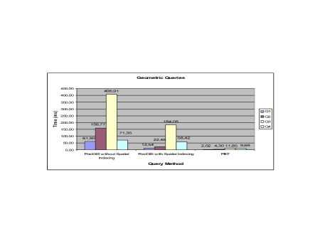
Figure 19: Execution time for geometric queries.

For tests of type (c), we selected four geometric aggregation queries that compute aggregations over the result of some geometric condition which involves the intersection between different combinations of layers. Table 5 depicts the expressions for these queries.

Query	Method	Code
Q5: Total number of rivers along with the total number of volcanoes in California	PostGIS without spatial indexing	SELECT count(DISTINCT river.id), count(DISTINCT volcano.id) FROM volcano, river, state WHERE state=’California’ AND contains( state.geometry, river.geometry) AND contains( state.geometry, volcano.geometry)
	PostGIS with spatial indexing	SELECT count(DISTINCT river.id), count(DISTINCT volcano.id) FROM volcano, river, state WHERE state=’California’ AND river.geometry && state.geometry AND volcano.geometry && state.geometry AND contains( state.geometry, river.geometry) AND contains( state.geometry, volcano.geometry)
	PIET	SELECT count(DISTINCT p1.river), count(DISTINCT p2.volcano) FROM gis_pre_linestring_3 p1, gis_pre_point_4 p2, state s WHERE p1.state = p2.state AND s.state= ’California’ AND p2.state = s.ID
Q6: Average elevation of volcanoes by state	PostGIS without spatial indexing	SELECT avg(elev), state.ID FROM volcano, state WHERE contains(state.geometry, volcano.geometry) GROUP BY state.ID
	PostGIS with spatial indexing	SELECT avg(elev), state.ID FROM volcano, state WHERE volcano.geometry && state.geometry AND contains(state.geometry, volcano.geometry) GROUP BY state.ID
	PIET	SELECT avg(p1.elev), p2.state FROM gis_subp_point_1 p1, gis_pre_point_4 p2 WHERE p1.originalgeometryID = p2.volcano GROUP BY p2.state
Q7: Average elevation of volcanoes by state, only for states crossed by at least one river.	PostGIS without spatial indexing	SELECT avg(elev), state.Piet_ID FROM volcano, state WHERE contains(state.geometry, volcano.geometry) AND state.PIET_ID in (SELECT state.Piet_ID FROM state, river WHERE intersects(state.geometry, river.geometry) ) GROUP BY state.Piet_ID
	PostGIS with spatial indexing	SELECT avg(elev), state.Piet_ID FROM volcano, state WHERE contains(state.geometry, volcano.geometry) AND state.geometry && volcano.geometry AND state.Piet_ID in (SELECT state.Piet_ID FROM state, river WHERE intersects(state.geometry, river.geometry) AND state.geometry && river.geometry) GROUP BY state.PIET_ID
	PIET	SELECT avg(p1.elev), p2.state FROM gis_subp_point_9 p1, gis_pre_point_9 p2 WHERE p1.originalgeometryID = p2.volcano AND p2.state IN (SELECT state FROM gis_pre_linestring_10) GROUP BY p2.state
Q8: Total length of the part of each river which intersects states containing at least one volcano with elevation higher than 4300	PostGIS without spatial indexing	SELECT length(intersection(state.geometry, river.geometry)), river.Piet_ID FROM river, state WHERE intersects(state.geometry, river.geometry) AND state.Piet_ID in (SELECT state.Piet_ID from state, volcano WHERE contains(state.geometry, volcano.geometry) AND volcano.elev ¿ 4300)
	PostGIS with spatial indexing	SELECT length(intersection(state.geometry, river.geometry)), river.Piet_ID FROM river, state WHERE river.geometry && state.geometry AND intersects(state.geometry, river.geometry) AND state.Piet_ID in (SELECT state.Piet_ID from state, volcano WHERE state.geometry && volcano.geometry AND contains(state.geometry, volcano.geometry) AND volcano.elev ¿ 4300
	PIET	SELECT SUM(length(p1.geometry)), p2.river FROM gis_subp_linestring_1 p1, gis_pre_linestring_3 p2 WHERE p1.uniqueID = p2.uniqueID and p1.originalgeometryID IN (SELECT p4.state FROM gis_subp_point_1 p3, gis_pre_point_4 p4 WHERE p3.originalgeometryID = p4.volcano AND p3.elev > 4300) group by p2.river

Table 5: Geometric aggregation queries.

Figure 20 shows the results. In this case, PIET ran faster that postGIS in queries Q5 through Q7 (ranging between four and five times faster, with respect to indexed PostGIS), but was outperformed in query Q8. This has to do, probably, with the complicated shape of the rivers and the number of carrier lines generated in regions with high density of volcanoes. Note however, execution times remain compatible with user needs. This could also be improved reducing the size of the grid only for high density regions, taking advantage of the flexibility of the grid partition strategy. Tests of similar queries with other maps have given clear advantages of Piet over R-tree indexing, for geometric aggregation (see http://piet.exp.dc.uba.ar/piet/index.jsp).

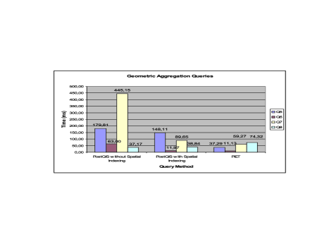
Figure 20: Execution time for geometric aggregation queries.

For the experiment (d), we ran the following three queries, and added a query region. We worked with two different query regions, shown in Figure 21. The queries were:
Q9: Average elevation of volcanoes by state, for volcanoes within the query region.
Q10: Average elevation of volcanoes by state only for the states crossed by at least one river, considering only volcanoes within the query region.
Q11: For each state show the total length of the part of each river which intersects it, only for states containing at least one volcano with elevation greater than 4300m.

The query expressions are of the kind of the ones given in tables 4 and 5, and we omit them for the sake of space. The results are shown in Figures 22 and 23. We denote query regions #1 and #2 the smaller and larger regions in Figure 21, respectively.

Figure 21: Query regions for geometric aggregation.

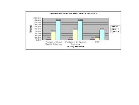
Figure 22: Geometric aggregation within query region # 1.

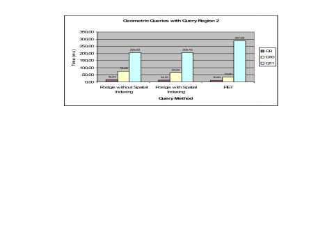
Figure 23: Geometric aggregation within query region # 2.

Figures 22 and 23 show the results. We can see that for the small query region, Piet still performs (about five times) better than indexed PostGIS. However, for the larger query region, for queries Q9 and Q10 Piet still delivers better performance, but for Q11 PostGIS with R-tree performs better (since this query is similar to Q8 above, the reasons of this result are likely to be the same). In the presence of query regions, Piet pays the price of the on-the-fly computation of the intersection between the query region and the sub-polygonization. It is worth mentioning that we indexed the overlayed sub-polygonization with an R-tree, with the intention of speeding-up the computation of the intersection between the query region and the sub-polygons, but the results were not satisfactory. Thus, we only report the results obtained without R-tree indexing. As a final remark, we implemented an optimization in Piet: we took advantage of the grid partition, in a way such that only the rectangles that intersect were the region boundaries were considered (i.e., the intersection algorithm only analyzes relevant rectangles) .
Precision of Piet Aggregation. We have commented above that, in some cases, we may lose precision in Piet when we aggregate measures defined over geometric objects. This problem appears when the object associated to measure to be aggregated does not lie within the query region (this also occurs in aR-trees, as we comment below). We ran a variation of query Q8: ‘ “length of rivers within a query region”. The boundary of the region is crossed by some rivers. We measure the difference between the lengths computed by Piet and by postGIS (exact result). The following table shows the results. The object ID represents the river being measured.

Object ID	Exact length	Computed by Piet	Diff.(%)
55	0.594427175	0.59442717	0
250	1.33177252	1.272456	4.7
251	0.2424391242	0.24243912	0
252	0.67318281	0.6731828	0
253	0.5103286611	0.510328661	0
254	0.0955072453	0.09550724	0
258	0.636150619	0.59679889	6.7

Note that for most of the rivers the precision is excellent, except for the ones with IDs 250 and 258, which are crossed by the query region. This could be fixed in Piet assuming the overhead of computing the exact length (inside the query region) of the segments that are intersected by the region boundaries.

Aggregation R-Trees. We implemented the aggregation R-tree (aR-tree), and ran two geometric aggregation queries, with or without a query region. In the latter case, Piet is still much better than the other two. However, in the presence of a query region, aR-tree and R-tree are between fifteen and twenty percent better than Piet. We report the results obtained running Q6: “Average elevation of volcanoes by state” (a geometric aggregation), and Q12: “Maximum elevation of volcanoes within a query region in California”. Figure 25 shows the six Minimum Bounding Rectangles (MBR) in the first level of the aR-tree, along with the query region for Q12. Figure 24 shows the results. The height of the aR-tree was h=2. We remark that the reported results were obtained in situations that favor aR-trees, since the queries deal with points. Aggregation over other kinds of objects that do overlap the query region may not be so favorable to aR-trees, given that base tables must be accessed, or otherwise, precision may be poor. The main benefit of aR-trees with respect to R-trees, come from pruning tree traversal when a region is completely included in an MBR, because, in this case, they do not need to reach the leaves of the index tree (because the values associated to all the geometries enclosed by the MBR have been aggregated). However, if this is not the case, the aR-tree should have to reach the leaves, as standard R-trees do, and the aR-tree advantages are lost. However, we want to be fair and remark that aR-trees may take advantage of the pre-aggregation methods as the size of the spatial database (and thus, the height of the tree) increases .

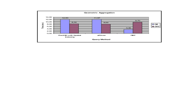
Figure 24: Piet vs aR-tree and R-tree

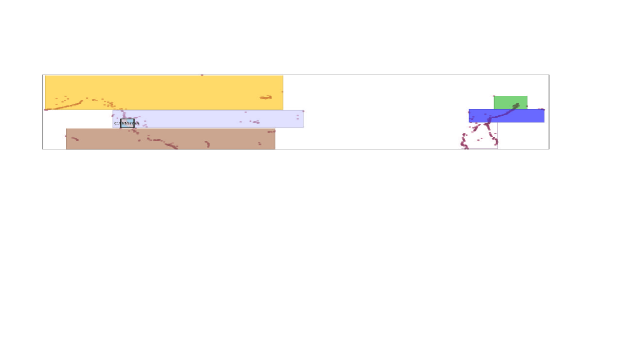
Figure 25: Minimum Bounding Rectangles and query region for the aR-tree (Query Q10).

Finally, we ran several tests of type (e). We already explained that GISOLAP-QL queries are composed of a GIS part and an OLAP part, expressed in MDX. The times for computing the GIS part (the SQL-like expression) were similar to the ones reported above. Note that in this case, there is no tool to compare Piet against to. We measured the total time for running a query, composed of the time needed for building the query, and the query execution time. As an example, we report the result of the following query:
Q14: Unit Sales, Store Cost and Store Sales for the products and promotion media offered by stores only in states containing at least one volcano.

The GISOLAP-QL query reads:

SELECT layer.state; FROM PietSchema; WHERE contains
(layer.state,layer.volcano,subplevel.point);
          |
SELECT {[Measures].[Unit Sales],

 [Measures].[Store Cost], [Measures].[Store Sales]}

ON columns, {([Promotion Media].[All Media],

[Product].[All Products])}

ON rows

FROM [Sales]

The query assembly and execution times are:

Assembly (ms)	Execution (ms)	Total (ms)
2023	60	2083

Discussion

Our results showed that the overlay precomputation of the common sub-polygonization appears as an interesting alternative to other more traditional methods, contrary to what has been believed so far [7]. We can summarize our results as follows:

• For pure geometric queries, Piet (i.e. overlay precomputation) clearly outperformed R-trees.

• For geometric aggregation performed over the entire map (i.e., when no query region must be intersected at run time with the precomputed sub-polygons), Piet clearly outperformed the other methods in almost all the experiments.

• When a query region is present, indexing methods and overlay precomputation deliver similar performance; as a general rule, the performance of overlay precomputation improves as the query region turns smaller. For small regions,

• Piet always delivered execution times compatible with user needs;

• The cost of integrating GIS results and OLAP navigation capabilities through the GISOLAP-QL query language (i.e.,merging the GIS part results with the MDX expression), is goes from low to negligible;

• It is worth commenting, although, that in the case of very large and complicated maps, with large query regions, aR-trees have the potential to outperform the other techniques.

• The class of geometric queries that clearly benefits from overlay precomputation can be easily identified by a query processor, and added to any existing GIS system in a straightforward way.

9 Topological Geometric Aggregation

In Section 4, we introduced summable queries to avoid integrals that may not be efficiently computable. At this point, the question that arises is: “What information do we store at the lowest level of the Geometric part?”. Should we store all the information about coordinates of nodes and corner points defining open convex polygons, or do we completely discard all coordinate information?. Depending on the purpose of the system, there are several possibilities. In this section, as another possible application of the concepts we studied in this paper, we will give a class of queries such that coordinate information is not needed for computing the answer.

A straightforward way of getting rid of the algebraic part of a GIS dimension schema, is to store the coordinates of nodes, end points of line segments and corner points of convex polygons. A closer analysis reveals that this information might not be necessary for all applications. For example, for queries about intersections of rivers and cities, or cities that are connected by roads or adjacent to rivers, we do not need coordinate information, but rather the topological information contained in the instance. Below, we characterize this class of queries.

To formalize the “depending on the purpose of the system” statement above, we introduce the concept of genericity of queries. Genericity of database queries was first introduced by Chandra and Harel [2]. A query is generic if its result is independent of the internal representation of the data. Later, this notion of genericity was applied to spatial databases [18, 28]. Paredaens et al. proposed a chain of transformation groups, motivated by spatial database practice, for which a query result could be invariant. From these groups, we will consider only the topological transformations of the plane.

Definition 9

(Genericity of a geometric aggregation query) Let $H$ be a group of transformations of $\mathbb{R}^{2}$. A geometric aggregation query $\mathrm{Q}$ is $H-$generic if and only if for any two input instances $G$ and $G^{\prime}$ of $\mathrm{Q}$ such that $G^{\prime}=h(G)$ for some transformation $h$ of $H$, $\mathrm{Q}$ returns the same result.     $\sqcap$$\sqcup$

Topological or isotopy-generic queries are useful genericity classes for geometric aggregation queries. For instance, query Q₂ from Example 5 is a topological geometric aggregation query. Another example is:

Q${}_{\mathrm{T_{1}}}$: Give me the number of states adjacent to Nevada.

If the purpose of the system is to answer topological queries, topological invariants [19, 27, 29] provide an efficient way of storing the information of one layer or the common sub-polygonization of several layers. This invariant is based on a maximal topological cell decomposition, which is, in general, hard to compute. Thus, in order to compute the topological invariant we will use our common sub-polygonization, which happens to be a refinement of the decomposition.

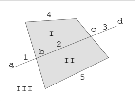
Figure 26: Topological information. Nodes are indicated by a, b, …, open curves by 1, 2, …. The faces are labelled I, II, ….

Figure 26 shows the topological information on the sub-polygonization of two layers, one containing a city and one containing a (straight) river. A topological invariant can be constructed from the maximal topological cell decomposition [19, 29] (or from the sub-polygonization), as follows. Cells of dimension $0$, $1$ and $2$ are called vertices, edges (these are different from line segments), and faces, respectively. The topological invariant is a finite structure consisting of the following relations: (1) Unary relations Vertex, Edge, Face and Exterior Face. The latter is a distinguished face of dimension $2$, i.e., the unbounded part of the complement of the figure; (2) A binary relation Regions providing, for each region name $r$ in the GIS instance the set of cells making up $r$; (3) A ternary relation Endpoints providing endpoints for edges; (4) A binary relation Face-Edge providing, for each face (including the exterior cell) the edges on its boundary; (5) A binary relation Face-Vertex providing, for each face (including the exterior cell) the vertices adjacent to it; (6) A $5-$ary relation Between providing the clockwise and counterclockwise orientation of edges incident to each vertex. For example, the relation Face-Edge will include the tuples $(I,2),(I,4);$ relation Face-Vertex will include $(I,b),(I,c);$ and relation between, the tuples $(\leftarrow,1,5,2)$ and $(\leftarrow,5,2,4),$ indicating the edges adjacent to vertex $b$ in counter-clockwise direction. Figure 27 shows the complete topological invariant. From the above, it follows that the relations representing the topological invariant can be used instead of the coordinates of the points in the Algebraic part, and the corresponding rollup functions. Further, the lowest level of a hierarchy in the geometric part will still contain (some of) the elements Node, OpolyLine and OPolygon (representing vertices, edges and faces, respectively). We also add the other relations, described above, as extra information attached to the hierarchy instance. This will suffice for answering summable topological queries.

Figure 27: The topological invariant for Figure 26.

Let us close our discussion with an example.

Example 11

Consider again query $\mathrm{Q}_{\mathrm{T_{1}}}$ above, using the topological invariant; To answer this query we need topological information about adjacency between polygons and lines (the Face-Edge relation). In order to be more clear, we will mention the domains of the geometry identifiers with different names. The query reads:

$\mathrm{Q}_{\mathrm{T_{1}}}\equiv\sum_{\mathrm{g_{id}}\in C_{T_{1}}}1,$ where

$$\halign{\hbox to\displaywidth{$\hfil\displaystyle#\hfil$}\cr 0.0pt{\hfil$\displaystyle\qquad C_{T_{1}}=\{g_{id}\in G_{Pg}~{}|\hfill{}\cr 0.0pt{\hfil$\displaystyle\hfill{}(\exists g_{1}\in G_{Pg})(\exists g_{2}\in G_{OPg})(\exists g_{3}\in G_{OPg})(\exists g_{4}\in G_{OPl})\hfill{}\cr 0.0pt{\hfil$\displaystyle\hfill{}(\exists p\in dom(\mathrm{State}))\hfill{}\cr 0.0pt{\hfil$\displaystyle\hfill{}(g_{1}\neq g_{id}~{}\land~{}\alpha_{L_{s},States}^{\mathrm{State}\rightarrow\mathrm{Pg}}(\mbox{p})=(g_{id})~{}\land\hfill{}\cr 0.0pt{\hfil$\displaystyle\hfill{}\alpha_{L_{s},States}^{\mathrm{State}\rightarrow\mathrm{Pg}}(\mbox{'Nevada'})=(g_{1})\hfill{}\cr 0.0pt{\hfil$\displaystyle\hfill{}\land f_{L_{s}}^{\mathrm{OPg}\rightarrow\mathrm{Pg}}(g_{2})=(g_{id})~{}\land\hfill{}\cr 0.0pt{\hfil$\displaystyle\hfill{}\land f_{L_{s}}^{\mathrm{OPg}\rightarrow\mathrm{Pg}}(g_{3})=(g_{1})\land\hfill{}\cr 0.0pt{\hfil$\displaystyle\hfill{}\land\mathrm{FaceEdge}(g_{2},g_{4})\land\mathrm{FaceEdge}(g_{3},g_{4})).\qquad\crcr}}}}}}}}}$$

What we have done here is finding all adjacency relationships using the $\mathrm{FaceEdge}$ relation. Thus, we just find all each open polygons that roll up to a polygon that represents a state other than Nevada; we also find out the polylines these open polygons are adjacent to. As we know the open polylines adjacent to the polygon representing Nevada, it is straightforward to find the states adjacent to Nevada and count them.     $\sqcap$$\sqcup$

10 Conclusion

In this paper we proposed a formal model that integrates GIS and OLAP applications in an elegant way. We also formalized the notion geometric aggregation, and identified a class of queries, denoted summable, which can be evaluated without accessing the Algebraic part of the GIS dimensions. We proposed to precompute the common sub-polygonization of the overlay of thematic layers as an alternative optimization method for evaluation of summable queries. We sketched a query language for GIS and OLAP integration, and described a tool, denoted PIET, that implements our proposal. We presented the results of our experimental evaluation (carried out over real-world maps), that show that precomputing the common sub-polygonization can successfully compete, for certain kinds of geometric queries, with traditional query evaluation methods. This is an important practical result, given that, up till now it has been thought that overlay materialization was not competitive against traditional search methods for GIS queries [7]. Our experiments show that for pure geometric queries, the precomputation of the overlay outperforms R-trees. The same occurs, in general, for geometric aggregation without on-the-fly computation. When the latter is required (v.g., where the aggregation must be performed over a dynamically defined query region, R-trees,in general, perform better than precomputed overlay. Nevertheless, we would like to remark that: (a) our implementation not only supports precomputed overlayed layers as query evaluation strategy, but R-trees and aR-trees as well; (b) the query execution times delivered were always more than acceptable values. We believe that these results are relevant, because they suggest that there is another alternative that query optimizers must consider. Finally, as a case study, we discussed topological aggregation queries, where geometric information has to be specified up to a topological transformation of the plane.

Our future work has two main directions: on the one hand, we believe there is still work to do in order to enhance the performance of the computation of the common subpolygonization, and overlay precomputation. On the other hand, we are looking forward to apply the concepts and models presented in this paper within the setting of Moving Objects Databases.

References

- [1] L. Cabibbo and R. Torlone. Querying multidimensional databases. In Proceedings of DBPL’97, pages 253–269, East Park, Colorado, USA, 1997.
- [2] A. K. Chandra and D. Harel. Computable queries for relational data bases. Journal of Computer and System Sciences, 21(2):156–178, 1980.
- [3] M. De Berg, M. Van Kreveld, M. Overmars, and O. Schwarzkopf. The Principles of Quantum Mechanics. Springer-Verlag, 2000.
- [4] P.A.M. Dirac. Computational Geometry: Algorithms and Applications. Oxford University Press, 1958.
- [5] GeoTools. The Java GIS Toolkit. GeoTools Home Page, 2005. http://www.geotools.org/.
- [6] A. Gutman. R-trees: A dynamic index structure for spatial searching. In Proceedings of SIGMOD’84, pages 47–57, 1984.
- [7] J. Han and M. Kamber. Data Mining, Concepts and Techniques. Morgan Kaufmann Publishers, 2001.
- [8] J. Han, N. Stefanovic, and K. Koperski. Selective materialization: An efficient method for spatial data cube construction. In Proceedings of PAKDD’98, pages 144–158, 1998.
- [9] V. Harinarayan, A. Rajaraman, and J. Ullman. Implementing data cubes efficiently. In Proceedings of SIGMOD’96, pages 205 – 216, Montreal, Canada, 1996.
- [10] J.M. Hellerstein, J.F. Naughton, and A. Pfeffer. Generalized search trees for database systems. In VLDB, pages 562–573, 1995.
- [11] R.F. Hoskins. Generalised functions. Ellis Horwood Series: Mathematics and its applications, John Wiley & Sons, 1979.
- [12] C. Hurtado, A.O. Mendelzon, and A. Vaisman. Maintaining data cubes under dimension updates. In Proceedings of IEEE/ICDE’99, pages 346–355, 1999.
- [13] C.S. Jensen, A. Kligys, T.B Pedersen, and I. Timko. Multidimensional data modeling for location-based services. VLDB Journal 13(1), pages 1–21, 2004.
- [14] JPivot. 2005. http://jpivot.sourceforge.net/.
- [15] Jump. The Jump Project, 2005. http://www.jump-project.org/.
- [16] R. Kimball. The Data Warehouse Toolkit. J.Wiley and Sons, Inc, 1996.
- [17] R. Kimball and M. Ross. The Data Warehouse Toolkit: The Complete Guide to Dimensional Modeling, 2nd. Ed. J.Wiley and Sons, Inc, 2002.
- [18] B. Kuijpers and D. Van Gucht. Genericity in spatial databases. In J. Paredaens, G. Kuper, and L. Libkin, editors, Constraint databases, chapter 12, pages 293–304. Springer-Verlag, 2000.
- [19] B. Kuijpers, J. Paredaens, and J. Van den Bussche. Lossless representation of topological spatial data. In Proceedings of SSD’95, volume 951 of Lecture Notes in Computer Science, pages 1–13. Springer, 1995.
- [20] B. Kuijpers and Alejandro Vaisman. A data model for moving objects supporting aggregation. In Proceedings of the First International Workshop on Spatio-Temporal Data Mining (STDM’07), Istambul, Turkey, 2007.
- [21] G. Kuper and M. Scholl. Geographic information systems. In J. Paredaens, G. Kuper, and L. Libkin, editors, Constraint databases, chapter 12, pages 175–198. Springer-Verlag, 2000.
- [22] W. Lehner. Modeling large OLAP scenarios. In EDBT’98: 6th International Conference on Extending Database Technology, pages 153–167, Valencia, Spain, 1998.
- [23] Mondrian. 2005. http://mondrian.sourceforge.net/.
- [24] OGC. Open Geospatial Consortium, 2005. http://www.opengeospatial.org/.
- [25] D. Papadias, P. Kalnis, J. Zhang, and Y. Tao. Efficient OLAP operations in spatial data warehouses. In Proceedings of SSTD’01, pages 443 – 459, 2001.
- [26] D. Papadias, Y. Tao, P. Kalnis, and J. Zhang. Indexing spatio-temporal data warehouses. In Proceedings of ICDE’02, pages 166–175, 2002.
- [27] C. H. Papadimitriou, D. Suciu, and V. Vianu. Topological queries in spatial databases. In Proceedings of PODS’96, pages 81–92. ACM Press, 1996.
- [28] J. Paredaens, J. Van den Bussche, and D. Van Gucht. Towards a theory of spatial database queries. In Proceedings of PODS’94, pages 279–288, New York, 1994.
- [29] J. Paredaens, G. Kuper, and L. Libkin, editors. Constraint databases. Springer-Verlag, 2000.
- [30] T.B Pedersen and N. Tryfona. Pre-aggregation in spatial data warehouses. Proceedings of SSTD’01, pages 460–480, 2001.
- [31] PostGIS. 2005. http://postgis.refractions.net/.
- [32] Postgres. Postgres SQL, 2005. http://www.postgresql.org/.
- [33] F. Rao, L. Zang, X. Yu, Y. Li, and Y. Chen. Spatial hierarchy and OLAP-favored search in spatial data warehouse. In Proceedings of DOLAP’03, pages 48–55, Louisiana, USA, 2003.
- [34] P. Rigaux, M. Scholl, and A. Voisard. Spatial Databases. Morgan Kaufmann, 2002.
- [35] S. Rivest, Y. Bédard, and P. Marchand. Modeling multidimensional spatio-temporal data warehouses in a context of evolving specifications. Geomatica, 55 (4), 2001.
- [36] S. Shekhar and S. Chawla. Spatial Databases: a Tour. Prentice Hall, 2003.
- [37] I. Vega López, R. Snodgrass, and B. Moon. Spatiotemporal aggregate computation: A survey. IEEE Transactions on Knowledge and Data Engineering 17(2), 2005.
- [38] M. F. Worboys. GIS: A Computing Perspective. Taylor&Francis, 1995.
- [39] L. Zang, , Y. Li, F. Rao, , X. Yu, and Y. Chen. An approach to enabling spatial OLAP by aggregating on spatial hierarchy. In Proceedings of DaWak’03, pages 35–44, Prague, Czech Republic, 2003.