Spectroscopy of two PN candidates in IC 10

Abstract

We present the results of the first spectroscopic observations of two planetary nebula (PN) candidates in the Local Group dwarf irregular galaxy IC 10. Using several spectral classification diagrams we show that the brightest PN candidate (PN 7) is not a PN, but rather a compact H ii region consisting of two components with low electron number densities. After the rejection of this PN candidate, the IC 10 planetary nebula luminosity function cutoff becomes very close to the standard value. With the compiled spectroscopic data for a large number of extragalactic PNe, we analyse a series of diagnostic diagrams to generate quantitative criteria for separating PNe from unresolved H ii regions. We show that, with the help of the diagnostic diagrams and the derived set of criteria, PNe can be distinguished from H ii regions with an efficiency of $\sim$99.6%. With the obtained spectroscopic data we confirm that another, 1$\aas@@fstack{m}$7 fainter PN candidate (PN 9) is a genuine PN. We argue that, based on all currently available PNe data, IC 10 is located at a distance 725${}^{+63}_{-33}$ kpc (distance modulus $\rm(m-M)=24.30^{+0.18}_{-0.10}$).

1 Introduction

The Local Group is an excellent laboratory for studies of galaxy evolution, providing us with a wide range of different galaxy types in a variety of environments. The star formation (SF) histories of Local Group galaxies can be obtained from color-magnitude diagrams of resolved stars (e.g., Aparicio & Gallart, 1995). Using this method it is possible to constrain the entire SF and chemical enrichment history of galaxies. However, the results are model-dependent, and should be compared with other, additional observational data which can be obtained for Local Group galaxies. One such complementary means of determining the SF and chemical evolution histories is a study of planetary nebulae (PNe), which can be used simultaneously as age, kinematics and metallicity tracers. The abundances from both H ii regions and PNe allow one to derive an approximate enrichment history for a galaxy from intermediate ages to the present day and permit abundance measurements at different locations. The latter, in turn, helps to test the homogeneity with which elements are distributed through a galaxy and, thus, the timescale for heavy element diffusion and mixing (Kniazev et al., 2005a, 2006a; Magrini et al., 2005a).

In this paper, we present new results of a PN study in the Local Group dwarf irregular galaxy IC 10, which is situated at low Galactic latitude ($b=-3\hbox{$.\!\!^{\circ}$ }3$). Estimates of the distance to IC 10 vary, including values of 830$\pm$110 kpc, based on observations of Cepheids (Saha et al., 1996); 660$\pm$66 kpc, based on Cepheids and tip of the red giant branch (RGB) stars (Sakai et al., 1999); and 741$\pm$37 kpc, based on a study of carbon stars (Demers et al., 2004). IC 10 is highly obscured, with $E_{B-V}=0.77\pm 0.07$ (Richer et al., 2001). With the position of IC 10 on the sky only $\simeq$18^∘ apart from M31, van den Bergh (2000) suggests that it may be a member of the M31 subgroup. The large number of H ii regions (Hodge & Lee, 1990) indicates that IC 10 is undergoing a massive episode of SF. Estimates of the intensity of SF were revised upward after many WR stars were discovered in IC 10 (Massey et al., 1992; Massey & Armandroff, 1995). This number of WR stars is remarkable for a galaxy of its size and is at least a factor of two higher than the density of such stars seen in any other Local Group galaxy. This fact led Massey & Armandroff (1995) to classify IC 10 as a starburst galaxy, the only such object in the Local Group. Richer et al. (2001) concluded that IC 10 should be considered a blue compact dwarf galaxy.

Sixteen PN candidates were identified in IC 10 by Magrini et al. (2003b) on the basis of both [O iii] and H$\alpha$+[N ii] continuum-subtracted images. No PNe were found very close to the center of this galaxy, presumably because of the presence of numerous extended HII regions covering a large fraction of the galaxy’s area. The distribution of m₅₀₀₇ magnitudes for all detected PN candidates looks unusual since the brightest one is $\sim$1$\aas@@fstack{m}$7 brighter than the next brightest. Observations and analysis of three of these PN candidates are presented below.

The paper is organized as follows. Section 2 gives a description of all observations and the data reduction. Our results are summarized in Section 3 and discussed in Section 4. Throughout the paper, for distance-dependent parameters we have assumed a distance to IC 10 of 740 kpc (Demers et al., 2004).

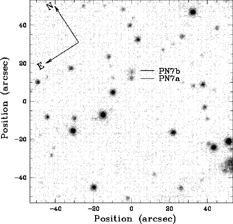
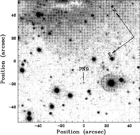
Figure 1: Co-added H$\alpha$ images obtained with the 6m telescope for PN 7 (top) and PN 9 (bottom) candidates in IC 10. Image orientations are shown with arrows. The black objects on the image correspond to bright sources. The long slits were aligned with the Y-axis in this coordinate system, crossing the abcissa at X=0. The positions of the observed PN candidates are marked. At the assumed distance of 740 Kpc, 1″ = 3.6 pc.

2 Spectral Observations and Data Reduction

Long-slit spectral observations were obtained with the SCORPIO multi-mode instrument (Afanasiev & Moiseev, 2005) installed in the prime focus of the SAO 6 m telescope (BTA), during two nights in November 2004. The VPH550g grism was used with the 2K$\times$2K CCD detector EEV 42-40, with an exposed region of 2048$\times$600 px. This gave a wavelength range $\sim$3500–7500 Å with $\sim$2.0 Å pixel^-1 and FWHM $\sim$12 Å along the dispersion direction. The scale along the slit was 0$\aas@@fstack{\prime\prime}$18 pixel^-1, with a total length of $\sim$2′and a slit width of 1″ . The coordinates for the observed PN candidates were taken from Magrini et al. (2003b). H$\alpha$ acquisition images were obtained before the spectroscopic observations in order to select optimal positions for the slit. In these images, the candidate PN 7 ($\alpha_{2000.0}$ = 00:20:22.22, $\delta_{2000.0}$ = 59:20:01.6 from Magrini et al. (2003b) appeared as an elongated object consisting of two regions: a starlike one (hereafter PN 7a) and an extended one (hereafter PN 7b). The slit was positioned to observe both of these simultaneously. Candidate PN 9 ($\alpha_{2000.0}$ = 00:20:32.08, $\delta_{2000.0}$ = 59:16:01.6) is a starlike source. Finding charts and the slit positions for our observations are shown in Figure 1. The exposure times used were 2$\times$15 min for PN 7 and 2$\times$20 min for PN 9, and the candidates were observed at airmasses of 1.8 and 1.1 respectively. For wavelength calibration, the object spectra were complemented by reference He–Ne–Ar lamp spectra. Bias and flat-field images were also acquired for a standard reduction of 2D spectra. The spectrophotometric standard star Feige 34 (Bohlin, 1996) was observed for flux calibration.

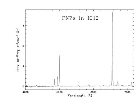
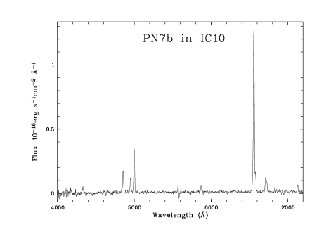
Figure 2: 1D spectra of PN candidates PN 7 and PN 9 in IC 10.

Reduction of all data was performed using the standard reduction systems MIDAS and IRAF. All cosmic ray hits were removed within MIDAS, while the IRAF package CCDRED was used for bad pixel removal, trimming, bias-dark subtraction, slit profile and flat-field corrections. To achieve accurate wavelength calibration, correction for distortion and tilt for each frame, sky subtraction and the correction for atmospheric extinction, the IRAF package LONGSLIT was used. Then, using the data on the spectrophotometric standard star, each 2D spectrum was transformed to absolute fluxes and one-dimensional spectra were extracted to obtain the total observed emission line fluxes.

All emission lines were measured using the MIDAS programs described by Kniazev et al. (2004). Briefly, they measure the continuum with the method of Shergin et al. (1996), derive robust noise estimates, and fit resolved lines with a single Gaussian superimposed on the continuum-subtracted spectrum. Some emission lines which were not sufficiently separated atr the given spectral resolution were fitted simultaneously as a blend of two or three Gaussian features. They include the H$\alpha$ $\lambda$6563 and [N ii] $\lambda\lambda$6548,6584 lines and the [S ii] $\lambda\lambda$6716,6731 lines. The quoted errors of single line intensities include the following components: (1) errors related to the Poisson statistics of line photon flux; (2) the error resulting from the measurement of the underlying continuum, which gives the dominant contribution to the errors on faint lines; (3) an additional error related to the goodness of fit for fluxes of blended lines; and (4) a term related to the uncertainty in the spectral sensitivity curve (5% for the presented observations), which constitutes the main contribution to the errors of the relative intensities of strong lines. All these components are added in quadrature, and the total errors have been propagated to calculate the errors of all subsequently derived parameters.

Table 1: Line intensities of the observed PN candidates in IC 10

	PN 7a			PN 7b			PN 9
$\lambda_{0}$(Å) Ion	$F$($\lambda$)/$F$(H$\beta$)	$I$($\lambda$)/$I$(H$\beta$)		$F$($\lambda$)/$F$(H$\beta$)	$I$($\lambda$)/$I$(H$\beta$)		$F$($\lambda$)/$F$(H$\beta$)	$I$($\lambda$)/$I$(H$\beta$)
4340 H$\gamma$	0.25$\pm$0.05	0.461$\pm$0.116		0.24$\pm$0.05	0.37$\pm$0.08		0.32$\pm$0.11	0.49$\pm$0.15
4861 H$\beta$	1.00$\pm$0.08	1.000$\pm$0.124		1.00$\pm$0.10	1.00$\pm$0.12		1.00$\pm$0.18	1.00$\pm$0.19
4959 [O iii]	1.46$\pm$0.12	1.263$\pm$0.109		0.65$\pm$0.07	0.58$\pm$0.07		4.35$\pm$0.53	3.61$\pm$0.65
5007 [O iii]	4.84$\pm$0.37	3.980$\pm$0.327		2.11$\pm$0.19	1.83$\pm$0.18		14.81$\pm$1.77	11.85$\pm$1.93
5876 He i	0.36$\pm$0.04	0.121$\pm$0.016		0.26$\pm$0.05	0.13$\pm$0.03		—	—
6548 [N ii]	0.37$\pm$0.04	0.069$\pm$0.009		0.31$\pm$0.05	0.11$\pm$0.02		0.35$\pm$0.12	0.11$\pm$0.04
6563 H$\alpha$	14.67$\pm$1.11	2.763$\pm$0.404		8.46$\pm$0.75	2.91$\pm$0.30		9.73$\pm$1.18	2.91$\pm$0.44
6584 [N ii]	1.13$\pm$0.14	0.209$\pm$0.031		0.97$\pm$0.10	0.33$\pm$0.04		1.22$\pm$0.23	0.36$\pm$0.08
6678 He i	0.12$\pm$0.02	0.021$\pm$0.004		—	—		—	—
6717 [S ii]	0.80$\pm$0.07	0.133$\pm$0.016		0.71$\pm$0.08	0.23$\pm$0.03		—	—
6731 [S ii]	0.58$\pm$0.06	0.096$\pm$0.013		0.49$\pm$0.06	0.15$\pm$0.02		—	—
7136 [Ar iii]	0.66$\pm$0.06	0.082$\pm$0.010		0.32$\pm$0.04	0.08$\pm$0.01		—	—
C(H$\beta$) dex	$\leq$2.10$\pm$0.04a			$\leq$1.35$\pm$0.07a			1.44$\pm$0.12
F(H$\beta$)b	7.50			4.7			0.66
EW(abs) Å	4.00			4.30			—
EW(H$\beta$) Å	140$\pm$4			142$\pm$7			—
$N_{\rm e}$(SII)(cm-3)	40$\pm$60			$\leq$10			—
Rad. vel. km s-1	$-$361$\pm$25			$-$355$\pm$34			$-$391$\pm$43
EB-V  mag	$\leq$1.43$\pm$0.03			$\leq$0.92$\pm$0.05			0.98$\pm$0.08
A5007  mag	$\leq$5.01$\pm$0.10			$\leq$3.22$\pm$0.17			3.43$\pm$0.29
a Note: PN 7a and 7b were not observed at the parallactic angle. See Section 3 for more details.
b Observed flux in units of 10-16 ergs s-1cm-2.

3 Results

The relative intensities (normalised to I(H$\beta$)) of all measured emission lines, as well as the derived extinction coefficient C(H$\beta$), the equivalent widths (EWs) of Balmer absorption lines, the measured flux of the H$\beta$ emission line, the measured heliocentric radial velocity, the electron density N_e, the calculated extinction $E_{B-V}=0.68\cdot C(H\beta)$, and the extinction value near $\lambda$5007 Å, $A_{5007}=3.5\cdot E_{B-V}$ (Cardelli et al., 1989) are given in Table 1. The final reduced 1D spectra are shown in Figure 2. The obtained values of $C$(H$\beta$) in all spectra are high and correspond respectively to the high derived values of $E_{B-V}$. Assuming a the Milky Way foreground extinction of $E_{B-V}\simeq 0.77$ in the direction of this galaxy (Richer et al., 2001), the internal extinction values $A_{5007}$ vary in the range of 0$\aas@@fstack{m}$5 to 2$\aas@@fstack{m}$3. The latter implies that IC 10 contains a considerable amount of internal dust, a conclusion supported by many previous studies. Because candidate PN 7 was observed at high airmass (1.8) but not at the parallactic angle, it is possible that some flux may have been lost in the blue and/or red parts of the spectra. As H$\alpha$ images were used to place objects on the slit, we most likely lost flux in the blue. Based on Filippenko (1982), we estimate that we might have lost $\sim 30\%$ in the spectral region of H$\beta$ and $\sim$50–60% in the spectral region of H$\gamma$. For this reason, the extinction values found for PN 7 and shown in Table 1 should be considered upper limits. Our measured total [O iii] $\lambda$5007 emission line fluxes for both observed candidates are about 20-30% lower than those presented by Magrini et al. (2003b). This is probably due to a combination of non-photometric conditions during our observations and the non-parallactic observation angle used for PN 7. Fortunately, the uncertain extinction determination for PN 7 does not affect the results presented in Section 4.

The derived radial velocities of PN 7a and PN 7b are close to each other, supporting the idea that both objects belong to the same complex. Their velocities are also close to the optical velocity of IC 10  V_hel = $-$348 km s^-1 (Huchra et al., 1999). Shostak & Skillman (1989) found that H i velocities in IC 10 range from $-$300 to $-$400 km s^-1. Comparison of PN 9’s position and its optical radial velocity with the 2D H i velocity distribution (Figure 7 from Shostak & Skillman, 1989) shows agreement to within the uncertainties of our velocity measurements. Thus, our radial velocities for both PN 7 and PN 9 support the idea that the observed PN candidates indeed belong to IC 10.

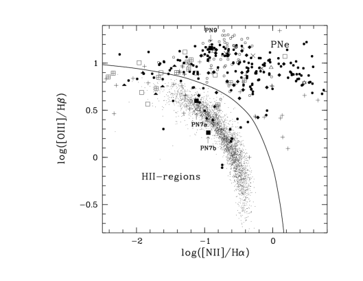
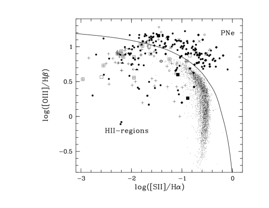
Figure 3: Classification diagrams for PNe/H ii galaxy separation. The SDSS DR1 strong emission-line H ii-galaxies from Kniazev et al. (2004) are plotted as dots. The data for extragalactic PNe are overplotted with different symbols: from M 31 as empty circles, from NGC 205 and M 32 as empty triangles, from Fornax, Sagittarius and NGC 147 as crossed squares, from NGC 5128 as crosses (x), from the SMC as pluses (+), from the LMC as filled diamonds, from Leo A and NGC 6822 as empty squares, from Sextans A as a star, from Sextans B as filled triangles, from M 33 as filled lozenges and the current data for IC 10 as filled squares. The positions of the observed IC 10 PN candidates are labeled in the upper panel. The points representing upper limits are shown with arrows in the lower panel. The solid line shows the models from Kewley et al. (2001) used for AGN/H ii galaxy separation.

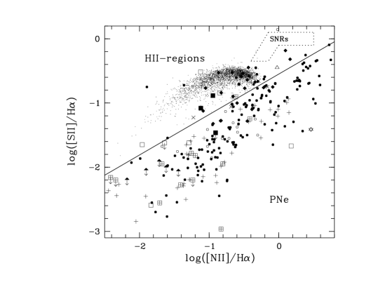
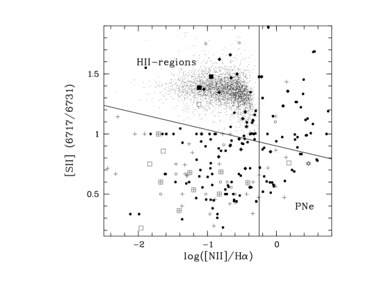
Figure 4: Classification diagrams for PNe/H ii galaxy separation. The symbols are the same as in Figure 3. The points representing upper limits are shown with downward arrows. The solid lines show graphically the criteria for PNe/H ii separation that were used in this work. See Section 4.1 for more details.

4 Discussion

4.1 PN or compact H ii region?

Most extragalactic PN candidates are point-like sources. The task of distinguishing between PNe and compact H ii regions in dwarf irregular and spiral galaxies is extremely difficult and cannot be accomplished with morphological criteria alone. Usually, the line ratio R=I([O iii] $\lambda$5007)/I(H$\alpha$ + [N ii] $\lambda\lambda$6548,6584) is used in searches for PN candidates with narrow-band imaging in H$\alpha$ and [O iii] $\lambda$5007 lines. A criterion of $\rm R>1.6$ for PN candidates was adopted by Ciardullo et al. (2002) after the analysis of a large sample of extragalactic PNe. However, it is well known that the ratio $\rm R$ is a function of the absolute magnitude of PNe, hence many extragalactic PN candidates can have $\rm R<1.6$ Magrini et al. (see, e.g., the list of PN candidates from 2003b, 2005b). Definitive classification/separation can only be performed with classification/diagnostic diagrams, after candidate spectra have been obtained. PNe spectra have the same emission lines as H ii regions, but the central stars of PNe are hotter than the OB stars in H ii regions, and the line intensity ratios are different for this reason. In addition, the electron densities in most PNe are higher than those in H ii regions. Empirical emission line diagrams are often used both to distinguish between different classes of ionized nebulae in the Galaxy (Sabbadin & D’Odorico, 1976; Sabbadin et al., 1977; García-Lario et al., 1991; Riesgo-Tirado & López, 2002; Magrini et al., 2003a; Riesgo-Tirado & López, 2006) and different types of emission-line galaxies (ELGs, e.g., Heckman, 1980; Baldwin et al., 1981; Veilleux & Osterbrock, 1987; Ugryumov et al., 1999). Unfortunately, unlike ELG classification based on such diagrams, to our knowledge there are no published quantitative criteria for distinguishing PNe from H ii regions. Analyses using the $\rm[\text{O\,\textsc{iii}}]\lambda 5007/H\beta$ ratio for classification purposes are absent from the literature as well, even though [O iii]$\lambda$5007 is the strongest line in most PN spectra.

To fill this gap and to derive quantitative criteria for the objective spectral classification of PN candidates, we first used a subsample of spectra of H ii regions (H ii galaxies) from the SDSS database (Kniazev et al., 2004). Their line intensity ratios are shown in Figures 3 and 4. These data cover very large ranges for a variety of emission line intensity ratios in H ii galaxies of different excitation types, and therefore can be used to define their loci properly. Secondly, we compiled from the literature a sample of extragalactic PNe with published spectra or emission line measurements. Data from the following galaxies were included: M 31 (Jacoby & Ford, 1986; Jacoby & Ciardullo, 1999; Kniazev et al., 2005b), M 33 (Magrini et al., 2003a), LMC and SMC (Aller, 1983; Monk et al., 1988; Boroson & Liebert, 1989; Meatheringham & Dopita, 1991a, b; Vassiliadis et al., 1992; Jacoby & Kaler, 1993; Dopita et al., 1993; Leisy & Dennefeld, 2006), Sextans A and Sextans B (Kniazev et al., 2005a; Magrini et al., 2005a), Leo A (Kniazev et al., 2005b), NGC 6822 (Richer & McCall, 2007), Fornax (Kniazev et al., 2006a, 2007), Sagittarius (Walsh, 1997; Zijlstra et al., 2006), NGC 147 (Gonçalves et al., 2007), M 32 (Jenner et al., 1979), NGC 205 (Richer & McCall, 1995), and NGC 5128 (Walsh et al., 1999). In cases for which measurements of [S ii] lines in PNe and PN candidates were not available, and for which we have data (PNe in Sextans B and PN 7 in IC 10), $2\sigma$ upper limits were calculated. These upper limits are shown as well with arrows. Our data for IC 10 were not used for criteria selection.

In total, we collected a sample of 259 different extragalactic PNe with measurements of all the emission line intensities we are considering: [O iii] $\lambda$5007, H$\beta$, H$\alpha$, [N ii] $\lambda$6584, and [S ii] $\lambda\lambda$6716,6731. We did not require separate measurements of the [S ii] $\lambda\lambda$6716,6731 lines for this sample, which we used for calculation of the overall selection efficiency. A subsample of 227 extragalactic PNe with resolved measurements of [S ii] $\lambda\lambda$6716,6731 was used to estimate the selection efficiency for criteria involving the use of the sulphur lines.

Our analysis has shown that it is possible to classify/separate almost all collected extragalactic PNe, if at least two (main) diagrams are used: log([O iii] $\lambda$5007/H$\beta$) vs.  log([N ii] $\lambda$6584/H$\alpha$) and log([S ii] $\lambda\lambda$6716,6731/H$\alpha$) vs.  log([N ii] $\lambda$6584/H$\alpha$). However, it is worth noting that most of these PNe can easily be separated with only the first diagram, which utilizes the strongest emission lines easily detectable in both PNe and H ii regions. It is clearly seen in the top panel of Figure 3 that most PNe are located in the same area as AGNs and can be easily distinguished with the model track of Kewley et al. (2001), often used for AGN/H ii segregation (see, e.g., Kniazev et al., 2004). The demarcation line from this model is shown as a solid line in Figure 3. We use this to construct the first quantitative criterion for the PNe selection:

$${\rm\log{([\text{O\,\textsc{iii}}]/H\beta)}\geq(0.61/\log{([\text{N\,\textsc{ii}}]/H\alpha)}-0.47)+1.19}$$ (1)

This allows us to identify 76% of all objects from the compiled list as PNe. However, the subsample of PN in Leo A, four PNe in Sextans B, the PN 7a and PN 7b candidates in IC 10 and some PNe candidates from M33, LMC and SMC form a locus in the area of H ii regions, so that other classification diagrams must be used to separate them. The use of the diagram log([O iii] $\lambda$5007/H$\beta$) vs.  log([S ii] $\lambda\lambda$6716,6731/H$\alpha$) (bottom panel of Figure 3) and the Kewley et al. (2001) model’s demarcation line

$${\rm\log{([\text{O\,\textsc{iii}}]/H\beta)}\geq(0.72/\log{([\text{S\,\textsc{ii}}]/H\alpha)}-0.32)+1.30}$$ (2)

does not help, since more PNe appear in the region of H ii compared with those found in the diagram log([O iii] $\lambda$5007/H$\beta$) vs.  log([N ii] $\lambda$6584/H$\alpha$). The classification efficiency of criterion (2) for our compiled PNe sample is only 62%. Thus we did not use the classification diagram log([O iii] $\lambda$5007/H$\beta$) vs.  log([S ii] $\lambda\lambda$6716,6731/H$\alpha$) in any further analysis.

The separation of supernova remnants (SNRs) is outside the scope of the current study. However, we suggest that most SNRs can also be distinguished with the use of the diagram log([O iii] $\lambda$5007/H$\beta$) vs.  log([N ii] $\lambda$6584/H$\alpha$), the model lines from Kewley et al. (2001), and the addition of model lines for LINER selection from Veilleux & Osterbrock (1987) and Baldwin et al. (1981), as was demonstrated in Kniazev et al. (2004). The latter is possible since both LINERs and SNRs have significant emission contributions from shock excitation. All such objects are located below the line corresponding to criterion (1). The locus of SNRs found in M 33 (Magrini et al., 2003a) supports this conclusion.

The diagram log([S ii] $\lambda\lambda$6716,6731/H$\alpha$) vs.  log([N ii] $\lambda$6584/H$\alpha$) (shown in the top panel of Figure 4), can be used as an additional diagnostic for the identification of PNe. From the analysis of our compiled PN data we have found that, with the use of only the criterion:

$${\rm\log{([\text{S\,\textsc{ii}}]/H\alpha)}\leq 0.63\cdot\log{([\text{N\,\textsc{ii}}]/H\alpha)}-0.55}$$ (3)

83% of our PNe can be recovered. However, with the combined use of criteria (3) and (1), 99% of PNe can be distinguished from H ii regions (i.e., all but two cases). Any analysed object is classified as a PN if it is located in the PNe locus according to at least of one of the cited criteria. It should be noted that, for many extragalactic PNe the detection of [S ii] $\lambda\lambda$6716,6731 lines is difficult, since the ratio I([S ii] $\lambda\lambda$6716,6731)/I(H$\beta$) is typically $\sim$0.5–5%. However, upper limits for this line ratio can be successfully used in this situation, similar to the cases of the PNe from Sextans B and the candidate PN 9 in IC 10. This second criterion is also very useful for rejecting possible SNRs, which fill the locus shown with the dashed line in the top panel of Figure 4.

The last classification diagram we considered is the relation between the flux ratio of the two lines of the [S ii] $\lambda$6716/$\lambda$6731 doublet and that of the flux ratio of the [N ii] $\lambda$6584 and H$\alpha$ lines: [S ii] $\lambda$6716/$\lambda$6731 vs.  log([N ii] $\lambda$6584/H$\alpha$). This is shown in the bottom panel of Figure 4. The criteria below

$${\rm[\text{S\,\textsc{ii}}]\lambda 6716/\lambda 6731\leq-0.135\cdot\log{([\text{N\,\textsc{ii}}]/H\alpha)}+0.90}\\$$ (4)

$${\rm\log{([\text{N\,\textsc{ii}}]/H\alpha)}\geq-0.25}$$ (5)

select 81% of PNe that have their [S ii] $\lambda\lambda$6716,6731 lines measured separately. With a combination of criteria (1) and (3), only one more PN is selected and the total selection efficiency reaches 99.6%. Just one PN from our compiled list, MCMP49 in M 33 (Magrini et al., 2003a), cannot be identified as a genuine PN using all the diagrams.

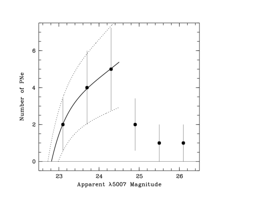
Figure 5: PNLF for the PN candidates in IC 10, excluding PN 7. The data have been binned in 0$\aas@@fstack{m}$6 intervals. The solid curve represent the best-fitting “universal” PNLF (Ciardullo et al., 1989) obtained for the data points. The dotted curves represent the best-fitting “universal” PNLFs obtained for the data points with $\pm 1\sigma$ errors.

4.2 On the brightest PN in IC 10 and its distance

The IC 10 candidate PN 9 observed in this work can be confidently classified as a true PN according to both criteria (1) and (3). However, according to all classification diagrams shown in Figures 3 and 4, IC 10 candidates PN 7a and PN 7b, cannot be selected as PNe and for this reason were finally classified as compact H ii regions. An additional reason to believe that PN 7a and PN 7b are H ii regions is the detection of continuum in their spectra (see Figure 2).

The absolute magnitude cutoff of the PNe [O iii] $\lambda$5007 luminosity function (PNLF) is considered to be constant in large galaxies with a large population of PNe, and is equal to $M_{*5007}=$-$4\aas@@fstack{m}47$ (Ciardullo et al., 2002). For dwarf galaxies, this cutoff is likely shifted towards the fainter magnitudes as a function of the galaxy mass and the population size (Méndez et al., 1993). Dopita et al. (1992) also examined the effects of metallicity on the luminosity of the brightest PN. According to their models, the variation of the cutoff magnitude $M_{*5007}$ with oxygen abundance is described by the relation

$${\rm\Delta M_{*5007}=0.928\cdot[O/H]^{2}+0.225\cdot[O/H]+0.014},$$ (6)

where [O/H] is the system’s logarithmic oxygen abundance referenced to the solar value 12+log(O/H) = 8.87 (Anders & Grevesse, 1989). Ciardullo et al. (2002) studied the accuracy of $M_{*5007}$ and found that $M_{*5007}=$-$4\aas@@fstack{m}47\pm 0.05$ after the correction for metallicity using equation (6).

The brightest PNe absolute magnitudes should be reasonably close to M_∗5007. With PN 7, the brightest candidate in IC 10 from Magrini et al. (2003b), M_∗5007 for this galaxy can be calculated as $-5\aas@@fstack{m}34$, where for candidate PN 7 $m_{5007}=21\aas@@fstack{m}71$ (Magrini et al., 2003b), $A_{5007}=2\aas@@fstack{m}70$, assuming background extinction of $E_{B-V}=0.77$ (Richer et al., 2001; Hunter, 2001) and a distance modulus $\rm(m-M)$ = 24.35 (Demers et al., 2004). Adopting the value of 12+$\log$(O/H) = 8.19, [O/H] = $-$0.68 and $\Delta M_{IC10,*5007}$ = 0.29, respectively for IC 10 we expect the ‘corrected’ cutoff magnitude for the IC 10 PNLF to be $M_{*5007}=$-$4\aas@@fstack{m}18$. Thus, the calculated M_∗5007 for PN 7 appears $\sim$1$\aas@@fstack{m}$15 brighter than the standard value.

After the rejection of the PN 7 candidate as an H ii region based on the results of our observations, the PNLF for PN candidates in IC 10 is shown in Figure 5, where data from Magrini et al. (2003b) have been binned into 0$\aas@@fstack{m}$6 intervals. Poisson $\pm 1\sigma$ error bars are shown for the detected number of PNe in these bins. We have fitted this PNLF with a “universal” PNLF (Ciardullo et al., 1989), taking only the brightest PNe (first three bins, eleven PNe in total) into account and using a uniform foreground extinction of $E_{B-V}=0.77$ (Richer et al., 2001; Hunter, 2001). The result of this fitting and Poisson errors are also shown in Figure 5. With this small sample we obtained the distance modulus $\rm(m-M)=24.30^{+0.18}_{-0.10}$ ( including the error in $M_{*5007}$), corresponding to a distance D = 725${}^{+63}_{-33}$ kpc; this is very close to the value from Demers et al. (2004). This distance modulus is also consistent with the recent estimate $\rm(m-M)=24.48\pm 0.18$ in Vacca et al. (2007), obtained from the study of individual RGB stars. With the PN data in hand, a distance to IC 10 of 950 Mpc (Massey & Armandroff, 1995; Hunter, 2001) seems implausible. The PNLF dip after the first three bins is likely a result of incompleteness, or could arise in a young population in which central star evolution proceeds very quickly (Jacoby & De Marco, 2002). Such a dip is also detected in the PNLFs in NGC 6822 (Leisy et al., 2005), the Small Magellanic Cloud and M 33 (Jacoby & De Marco, 2002; Ciardullo et al., 2004).

Of course, PN candidates, not confirmed PNe, were used for the PNLF calculation (except in the case of PN 9, which was confirmed in this paper), making this result for the IC 10 PNLF distance somewhat preliminary. However, all the bright PN candidates that were used for the PNLF fitting have $\rm R>1.6$ (Magrini et al., 2003b) and thus have a very high probability of being real PNe.

The calculated distance to IC 10 obviously depends on the extinction values used; higher extinction values would place IC 10 even closer to us. The total extinction value toward IC 10 is a combination of foreground (i.e., Galactic) extinction, and the extinction internal to IC 10 ; this latter quantity is quite uncertain, and for this reason only foreground extinction is usually considered (as we have done in this work). The great advantage of PNLF distance calculations (compared to other methods) is that, in principle, the total extinction along the line of sight can be calculated after proper spectral observations of PN candidates and calculations of C(H$\beta$) for each PN (Jacoby, Walker, & Ciardullo, 1990). For this reason further spectroscopic observations of other PN candidates in IC 10 are very important. On the other hand, total extinctions calculated using C(H$\beta$) for PNe have to be used carefully, since could be strongly affected by extinction in localised circumstellar material. For this reason we do not make further use of the extinction we derive from the spectrum of PN 9 in IC 10; instead, we plan to map the line-of-sight extinction in its neighbourhood through observations of nearby H ii regions.

5 Conclusions

In this paper we present the first results of follow-up spectroscopy of PN candidates in the Local Group starburst galaxy IC 10. Based on our data and the discussion above, we draw the following conclusions:

1. From the obtained spectral data and the emission line diagnostic diagrams we have found that the brightest candidate PN 7 from the list of Magrini et al. (2003b) is not a genuine PN, but rather a close pair of compact H ii regions. The calculated absolute magnitude M_∗5007 for PN 7 is about 1$\aas@@fstack{m}$15 brighter than the standard maximum value from the PN luminosity function expected at the approximate distance of IC 10.

2. We have found that PN 9, obtained from the same list of candidate PNe, is a true PN, and thus is the first confirmed PN in IC 10.

3. With the available PN candidate data, we estimate the PNLF distance to IC 10 as 725${}^{+63}_{-33}$ kpc, a distance modulus of $\rm(m-M)=24.30^{+0.18}_{-0.10}$.

References

- Afanasiev & Moiseev (2005) Afanasiev, V.L., & Moiseev, A.V. 2005, Astron. Lett., 31, 193
- Aparicio & Gallart (1995) Aparicio, A., & Gallart, C. 1995, AJ, 110, 2105
- Aller (1983) Aller, L.H. 1983, ApJ, 273, 590
- Anders & Grevesse (1989) Anders, E., & Grevesse, N. 1989, Geochim.Cosmochim.Acta, 53, 197
- Baldwin et al. (1981) Baldwin, J.A., Phillips, M.M.,& Terlevich R. 1981, PASP, 93, 5
- Bohlin (1996) Bohlin, R.C. 1996, AJ, 111, 1743
- Boroson & Liebert (1989) Boroson, T.A., & Liebert, J. 1989, ApJ, 339, 844
- Cardelli et al. (1989) Cardelli, J.A., Clayton, G.C., & Mathis, J.S. 1989, ApJ, 345, 245
- Ciardullo et al. (1989) Ciardullo, R., Jacoby, G.H., Ford, H.C., & Neill, J.D. 1989, ApJ, 339, 53
- Ciardullo et al. (2002) Ciardullo, R., et al. 2002, ApJ, 577, 31
- Ciardullo et al. (2004) Ciardullo, R., et al. 2004, ApJ, 614, 167
- Demers et al. (2004) Demers, S., Battineli, P. & Letarte, B. 2004, A&A, 424, 125
- Dopita et al. (1992) Dopita, M.A., Jacoby, G.H., & Vassiliadis, E. 1992, AJ, 389, 27
- Dopita et al. (1993) Dopita, M.A. et al. 1993, ApJ, 418, 804
- Filippenko (1982) Filippenko, A.V. 1982, PASP, 94, 715
- García-Lario et al. (1991) García-Lario, P., Manchado, A., Riera, A., Mampaso, A., & Pottasch, S.R. 1991, A&A, 249, 223
- Gonçalves et al. (2007) Gonçalves, D.R., Magrini, L., Leisy, P., & Corradi, R.L.M. 2007, MNRAS, 375, 715
- Heckman (1980) Heckman, T.M. 1980, A&A, 87, 152
- Hodge & Lee (1990) Hodge, P., & Lee, M.G. 1990, PASP, 102, 26
- Huchra et al. (1999) Huchra, J.P., et al. 1999, ApJS, 121, 287
- Hunter (2001) Hunter, D.A., 2001, ApJ, 559, 225
- Jenner et al. (1979) Jenner, D.C., Ford, H.C., & Jacoby, G.H. 1979, ApJ, 227, 391
- Jacoby & De Marco (2002) Jacoby, G.H., & De Marco , O. 2002, AJ, 123, 269
- Jacoby & Ford (1986) Jacoby, G.H., & Ford, H.C. 1986, ApJ, 304, 490
- Jacoby & Ciardullo (1999) Jacoby, G.H., & Ciardullo, R. 1999, ApJ, 515, 169
- Jacoby & Kaler (1993) Jacoby, G.H., & Kaler, J.B. 1993, ApJ, 417, 209
- Jacoby, Walker, & Ciardullo (1990) Jacoby, G.H., Walker, A.R., & Ciardullo, R. 1990, ApJ, 365, 471
- Kewley et al. (2001) Kewley, L.J., Dopita, M.A., Sutherland, R.S., Heisler, C.A., & Trevena, J. 2001, ApJ, 556, 121
- Kniazev et al. (2004) Kniazev, A.Y., Pustilnik, S.A., Grebel, E.K., Henry Lee, & Pramskij, A.G. 2004, ApJS, 153, 429
- Kniazev et al. (2005a) Kniazev, A.Y., Grebel, E.K., Pustilnik, S.A., Pramskij, A.G., & Zucker, D. 2005a, AJ, 130, 1558
- Kniazev et al. (2005b) Kniazev, A.Y., Grebel, E.K., Zucker, D., et al. 2005b, in Planetary Nebulae as Astronomical Tools, AIP Conf. Proc., eds. G. Stasínska & R. Szczerba, 804, 15
- Kniazev et al. (2006a) Kniazev, A.Y., Grebel E.K., Pramskij, A.G., & Pustilnik, S.A. 2006, Planetary Nebulae Beyond the Milky Way, edited by L. Stanghellini, J.R. Walsh and N. Douglas, ESO Astrophysics Sympisia, Springer, 257
- Kniazev et al. (2007) Kniazev A.Y., Grebel, E.K., Pustilnik, S.A., & Pramskij, A.G. 2007, A&A, 468, 121
- Leisy et al. (2005) Leisy, P., Corradi, R.L.M., Magrini, L. et al. 2005, A&A, 436, 437
- Leisy & Dennefeld (2006) Leisy, P., & Dennefeld, M. 2006, A&A, 456, 451
- Magrini et al. (2003a) Magrini, L., Perinotto, M., Corradi, R.L.M., & Mampaso, A. 2003a, A&A, 400, 511
- Magrini et al. (2003b) Magrini, L., et al. 2003b, A&A, 407, 51
- Magrini et al. (2005a) Magrini, L., et al. 2005a, A&A, 443, 115
- Magrini et al. (2005b) Magrini, L., et al. 2005b, MNRAS, 361, 517
- Massey & Armandroff (1995) Massey, P., & Armandroff, T.E. 1995, AJ, 109, 2470
- Massey et al. (1992) Massey, P., Armandroff, T.E., & Conti, P.S. 1992, AJ, 103, 1159
- Meatheringham & Dopita (1991a) Meatheringham, S.J., & Dopita, M.A. 1991a, ApJS, 75, 407
- Meatheringham & Dopita (1991b) Meatheringham, S.J., & Dopita, M.A. 1991b, ApJS, 76, 1085
- Méndez et al. (1993) Méndez, R.H., Kudritzki, R.P., Ciardullo, R., & Jacoby, G.H. 1993, A&A, 275, 534
- Monk et al. (1988) Monk, D.J., Barlow, M.J., & Clegg, R.E.S. 1988, MNRAS, 234, 583
- Richer & McCall (1995) Richer, M.G., & McCall, M.L. 1995, ApJ, 445, 642
- Richer et al. (2001) Richer, M.G., et al. 2001, A&A, 370, 34
- Richer & McCall (2007) Richer, M.G., & McCall, M.L., 2007, ApJ, 658, 328
- Riesgo-Tirado & López (2002) Riesgo-Tirado, H., & López, J.A. 2002, RevMexAA 12, 174
- Riesgo-Tirado & López (2006) Riesgo-Tirado, H., & López, J.A. 2006, RevMexAA 42, 47
- Sabbadin & D’Odorico (1976) Sabbadin, F., & D’Odorico, S. 1976, A&A, 49, 119
- Sabbadin et al. (1977) Sabbadin, F., Minello, S., & Bianchini, A. 1977, A&A, 60, 147
- Saha et al. (1996) Saha, A., Hoessel, J.G., Krist, J., & Danielson, G.E. 1996, AJ, 111, 197
- Sakai et al. (1999) Sakai, S., Madore, B.F., & Freedman, W.L. 1999, ApJ, 511, 671
- Shergin et al. (1996) Shergin, V.S., Kniazev, A.Y., & Lipovetsky, V.A. 1996, Astronomische Nachrichten, 317, 95
- Shostak & Skillman (1989) Shostak, G.S., & Skillman, E.D. 1989, A&A, 214, 33
- Ugryumov et al. (1999) Ugryumov A.V., et al. 1999, A&AS, 135, 511
- Vacca et al. (2007) Vacca, W.D., Sheehy, C.D., Graham, J.R. 2007, ApJ in press (astro-ph/0701628)
- van den Bergh (2000) van den Bergh, S. 2000, in The Galaxies of the Local Group (Cambridge: Cambridge University Press), 177
- Vassiliadis et al. (1992) Vassiliadis, E., Dopita, M.A., Morgan, D.H., & Bell, J.F. 1992, ApJS, 83, 87
- Veilleux & Osterbrock (1987) Veilleux, S., & Osterbrock, D.E. 1987, ApJS, 63, 295
- Walsh (1997) Walsh, J.R., Dudziak, G., Minniti, D., & Zijlstra, A.A. 1997, ApJ, 487, 651
- Walsh et al. (1999) Walsh, J.R., et al. 1999, A&A, 346, 753
- Zijlstra et al. (2006) Zijlstra, A.A., Gesicki, K, Walsh, J.R., Péquignot, D., van Hoof, P.A.M., & Minniti, D. 2006, MNRAS, 369, 875