On dynamical tunneling and classical resonances

Abstract

This work establishes a firm relationship between classical nonlinear resonances and the phenomenon of dynamical tunneling. It is shown that the classical phase space with its hierarchy of resonance islands completely characterizes dynamical tunneling and explicit forms of the dynamical barriers can be obtained only by identifying the key resonances. Relationship between the phase space viewpoint and the quantum mechanical superexchange approach is discussed in near-integrable and mixed regular-chaotic situations. For near-integrable systems with sufficient anharmonicity the effect of multiple resonances i.e., resonance-assisted tunneling can be incorporated approximately. It is also argued that the, presumed, relation of avoided crossings to nonlinear resonances does not have to be invoked in order to understand dynamical tunneling. For molecules with low density of states the resonance-assisted mechanism is expected to be dominant.

I Introduction

Intramolecular vibrational energy redistribution (IVR) in a molecule, from an initially prepared nostationary state, is at the heart of chemical reaction dynamics. The timescales and mechanisms involved in this process of energy flow have been investigated in great detail by experiments and theoryivrrev . Although considerable progress has been made over the years there are many aspects of this phenomenon whose understanding still eludes us. Nevertheless it is expected that there is a part of the IVR mechanism which can be usefully understood based on classical dynamics alone and there is a part of IVR which is intrinsically quantum mechanical. Both classical and quantum mechanisms coexist in a given molecule and give rise to complicated spectral patterns and splittings.

It is now well established that a specific overtone excitation in a molecule will undergo IVR if the initial nonstationary state, zeroth-order bright state (ZOBS), is coupled to other ’dark’ zeroth-order states via strong anharmonic resonances. In such cases classical dynamics, at various levels of detail and sophistication, can provide useful insights into the timescales and mechanisms of IVRclivr . On the other hand if the ZOBS is not close to any resonance then classically one expects no IVR and hence no fractionation of spectral lines. However, it is still possible for IVR to occur via quantum routes. In other words the initial state will mix with other states giving rise to spectral splittings and, possibly, complicated eigenstates. Since the mixing is classically ’forbidden’ it would be appropriate to associate some kind of tunneling with such quantum routes to energy flow. Indeed such a suggestion was made over two decades agodavhel and the term ’dynamical tunneling’ was coined. The notion of tunneling is meaningless without one form of a barrier or other and the term ’dynamical’ is prefixed to distinguish from the usual coordinate space tunneling through static potential barriers. The barriers in dynamical tunneling, in general, are more subtle to identify and exist in the phase space.

Dynamical tunneling can have important consequences for the interpretation of molecular spectra since the fingerprints of IVR are spectrally encoded in the form of intensities and splittings. Traditionally dynamical tunneling in the molecular context has been associated with the occurence of local modelocal stretches in symmetric molecules. However it is important to emphasize that the concept of dynamical tunneling is more general - any flow of quantum probability between regions which are classically disconnected is dynamical tunneling. The identification of classically disconnected regions requires the knowledge of the phase space topology and hence it is not very surprising that dynamical tunneling is inevitably linked to the underlying classical dynamics. In the context of local mode doublets in symmetric systems important work by Jaffé and Brumerjafbrum and Kellmankell provided classical phase space perspectives on the normal to local transition. One of the reasons for the interest in the near-degenerate local doublets has to do with their long lifetimes. Thus provided one can experimentally prepare a high overtone, of say the OH-stretch in H₂O, then the extremely small splitting provides a large window of time to perform mode selective chemistry. The main problem with such an idea is that at such high vibrational excitations other Fermi resonances and rovibrational interactions could destroy the degeneraciesquackarpc . We hope to shed some light on these issues in this work wherein the system of interest does exhibit close degeneracies despite multiple resonances and a classical phase space which is mixed regular-chaotic. Interestingly, similar issues have been addressed in the context of the existence of discrete breathers in a network of nonlinear oscillatorsdb .

One of the earliest examples in symmetric systems are the local mode doublets observed in the water molecule which were explained by Lawton and Child as due to dynamical tunnelinglawch . The experimentskerst of Kerstel et.al. on unusally slow (hundreds of picoseconds) intramolecular vibrational relaxation of CH-stretch excitation in (CH₃)₃CCCH molecule has also been ascribed to dynamical tunneling by Stuchebrukhov and Marcusstuma1 . In this case the extremely slow IVR out of the CH-stretch is an instance of dynamical tunnneling in nonsymmetric systems. In a later experiment McIlroy and Nesbitt noted multiquantum state mixing due to very small couplings (0.1 cm^-1 or less) in the CH stretch excitation in propynemcnes . Recent experiments have shown similar effects in the CH-stretch excitations of triazinetri and 1-butynebut and there are reasons to expect dynamical tunneling to manifest in general rovibrational spectramcd ; kel ; hart ; lehkk ; orti .

Much of the theoretical understanding of dynamical tunneling has come about from the analysis of bent triatomic ABA molecules. The focus primarily has been on vibrations and this work is no expception in this regard. However we note the important work by Lehmannlehkk wherein the nontrivial effects arising due to coupling between local modes and rotations are studied in detail. Davis and Hellerdavhel emphasized a phase space picture and implicated classical resonances in the phase space as the agents of dynamical tunneling. In this approach classical trajectories trapped in one region of the phase space were imagined to be separated by dynamical barriers, due to the resonances, from symmetrically equivalent regions of the phase space. The degeneracy is then broken by dynamical tunneling. A clear demonstration of the role of isolated resonances was provied by Ozorio de Almeida as wellozo . A slightly different picture was provided by Sibert, Reinhardt and Hynessihy in their work on energy flow and local mode splittings in the water molecule. The setting was again in terms of classical nonlinear resonances but the dynamical barrier was identified in angle space as opposed to in action space. Later Hutchinson, Sibert and Hyneshusihy provided an explanation for the quantum energy flow in terms of high order perturbation theory. Stuchebrukhov and Marcusstuma2 reanalyzed the ABA system in terms of chains of off-resonance virtual states (”vibrational superexchange”) connecting any two degenerate local mode states. An important result was the equivalence between the vibrational superexchange approach and the usual WKB expression for splittings in a doublewell system. This equivalence between perturbative and the WKB approaches was shown for a classically integrable case. Demonstration of such an equivalence in more general situations is an open problem. Despite seemingly different approaches a crucial ingredient to any description of dynamical tunneling involves the various anharmonic resonances. Depending on the level of excitation the underlying phase space can exhibit several (near) equivalent regions separated by nonlinear resonances (near-integrable phase space) or chaos (mixed phase space). For large molecules with sufficient density of states, in the near-integrable regime, Heller has conjecturedhel9599 that a nominal 10^-1-10^-2 cm^-1 broadening of spectroscopically prepared zeroth-order states is due to dynamical tunneling between remote regions of phase space facilitated by distant resonances.

The aforementioned conjecture is based on the notion that phase space is the correct setting for an understanding of dynamical tunneling. It is thus natural to expect the splittings to be sensitive to the structure of the phase space. It also follows that given the phase space structure one ought to be able to compute the associated splittings. General forms for splittings cannot be written down easily since explicit forms of the dynamical barriers in the phase space, seperating quantum states localized in distant regions of the phase space, can only be provided upon identification of the key nonlinear resonances. This is also tanatamount to identifying the mechanism of dynamical tunneling and hence IVR. Two factors make this a difficult problem. Firstly, our understanding of global structure of multidimensional classical phase space is still in its infancy. Thus without a global view of the phase space at energies corresponding to the doublets it is difficult to identify the main nonlinear resonances and perhaps the presence of appreciable stochastic layers. Secondly, and related to the first factor, important work over the last decade has established that dynamical tunneling is sensitive not only to the nonlinear resonancesrat1 ; rat2 but also to the classical stochasticitycat . In the near-integrable regimes dynamical tunneling can be enhanced by many orders of magnitude due to the various nonlinear resonances. This is called as resonance-assisted tunneling and it has been suggestedelt that the nonlinear resonances play an important role in mixed phase space scenario as well. In cases where an appreciable chaotic region separates the two symmetry related regular zones one has the phenomenon of chaos-assisted tunneling. The hallmark of chaos-assisted tunneling is the erratic fluctuations of the splittingscat due to ’chaotic’ states having nonzero overlaps with the regular doublets. In particular the splittings show algebraic dependence on $\hbar$ as opposed to the integrable $\exp(-1/\hbar)$ scaling. Experimentsexpt on a wide variety of systems have highlighted the role of the phase space structures in dynamical tunneling.

Is the evidence for the sensitivity of dynamical tunneling to the phase space structures already present in the molecular spectra? The answer to this question, apart from a fundamental viewpoint, is also potentially relevant to mode-specific chemistry and control. In this context, it is significant to note that most of the earlier works in the molecular context have focused on dynamical tunneling where only one resonance was involved with no chaos. A notable exception is the work of Davis and Hellerdavhel wherein a hint to the role played by classical chaos was provided. The sensitivity of dynamical tunneling to the underlying phase space structure can have important ramifications in the molecular context. Phase space of molecular systems at higher energies, corresponding to high overtone transitions, are typically a mixture of regular and chaotic regions. The presence of stochasticity can lead to the dynamical tunneling being enhanced (or suppressed) by several orders of magnitude and hence highly mixed states and complicated spectral patterns. Even in the near-integrable regimes tiny induced resonances can arise as a result of the primary resonances which can enhance or suppress dynamical tunneling between symmetry related modes. Alternatively, molecule-field interactions canmfield lead to creation (destruction) of nonlinear resonances which can lead to significant enhancement or supression of energy flow.

The purpose of this work is to establish the role of classical resonances in the near-integrable phase space for dynamical tunneling and the nontrivial effect of higher order induced resonances and perhaps chaos. We focus on the symmetric case in this work but the role played by the nonlinear resonances is expected to hold in the nonsymmetric situations as well. In the near-integrable regime it is possible for more than one nonlinear resonance zone to manifest in the phase space. In such instances the single rotor pictureozo ; sihy is not sufficient to account for dynamical tunneling. Yet it is shown that hopping across the various resonance islands is an approximate picture that yields qualitative (and perhaps quantitative) insights into the splitting patterns. We start by motivating the model Hamiltonian in section II. In section III the concept of dynamical tunneling and quantum viewpoints are illustrated. The phase space viewpoint and relations to the quantum viewpoint are discussed in section IV by focusing on specific cases. In section IV.2 two issues regarding avoided crossings and influence of very small induced resonances are addressed briefly. Complications due to multiple resonances in the near-integrable limit and the resulting resonance-assisted tunneling are illustrated in section IV.3. The possibility of chaos-assisted tunneling occuring in the system is explored in section IV.4. A brief summary is provided in section V.

II Model Hamiltonian

As discussed in the introduction attempts to understand dynamical tunneling, from a classical phase space viewpoint, in three or more degrees of freedom systems is ambitious without studying the detailed correspondence in lower dimensions with multiple resonances. In this regard the effective spectroscopic Hamiltonian for water due to Baggottbagg provides a good model system. The Hamiltonian is given by

$$\hat{H}_{C}=\hat{H}_{0}+g^{\prime}\hat{V}^{(12)}_{1:1}+\gamma\hat{V}^{(12)}_{2:2}+\frac{\beta}{2\sqrt{2}}(\hat{V}^{(1b)}_{2:1}+\hat{V}^{(2b)}_{2:1})$$ (1)

with, $g^{\prime}=g+\lambda^{\prime}(n_{1}+n_{2}+1)+\lambda^{\prime\prime}n_{b}$ and

$$\hat{H}_{0} = \omega_{s}(n_{1}+n_{2})+\omega_{b}n_{b}+x_{s}(n^{2}_{1}+n^{2}_{2})$$ (2)

$$+ x_{b}n^{2}_{b}+x_{sb}n_{b}(n_{1}+n_{2})+x_{ss}n_{1}n_{2}$$

describing the anharmonic local stretches $(1,2)$, and bend $(b)$. The various parameter values are $\omega_{s}=3885.57,\omega_{b}=1651.72,x_{s}=-81.99,x_{b}=-18.91,x_{sb}=-19.12$ and, $x_{ss}=-12.17$ cm^-1. The $j^{th}$ mode occupancy is $n_{j}=a^{\dagger}_{j}a_{j}$ with $(a^{\dagger}_{j},a_{j})$ being the harmonic oscillator creation and destruction operators. The perturbations, anharmonic resonances,

$$\hat{V}^{(ij)}_{p:q}=(a^{\dagger}_{i})^{q}(a_{j})^{p}+(a^{\dagger}_{j})^{p}(a_{i})^{q}$$ (3)

connect zeroth-order states $|{\bf n}\rangle$, $|{\bf n}^{\prime}\rangle$ with $|n_{i}^{\prime}-n_{i}|=q$ and $|n_{j}^{\prime}-n_{j}|=p$. The strengths of the resonances are $g=-56.48,\lambda^{\prime}=3.02,\lambda^{\prime\prime}=-0.18,\gamma=-0.91$, and $\beta=26.57$ cm^-1. In order to perform detailed studies on the above Hamiltonian in this work we also analyze subsystems obtained by retaining specific resonances. These subsystems, denoted by $A$ and $B$, are described by the Hamiltonians $H_{A}=H_{0}+\beta(V^{(1b)}_{2:1}+V^{(2b)}_{2:1})$ and $H_{B}=H_{A}+\gamma V^{(12)}_{2:2}$ respectively. The full system with all the resonances will be denoted by $C$. The reason for this specific choice of subsystems has to do with the fact that classically $H_{A}$ and $H_{B}$ exhibit near-integrable dynamics whereas $H_{C}$ has mixed regular-chaotic dynamics. $\hat{H}$ is effectively two dimensional due to the existence of the conserved polyad $P=(n_{1}+n_{2})+n_{b}/2$ i.e., $[\hat{H},\hat{P}]=0$. Spectroscopic Hamiltonians can be obtained by a fit to the high resolution spectra or from a perturbative analysis of an existing high quality ab initio potential energy surfacejoy . In any case such Hamiltonians, and variants thereof, have proved quite useful in studying the highly excited vibrations of many small moleculesjacjpc . Couplings to rotations and large amplitude modes are certainly importantlehkk but a detailed phase space analysis of such general rovibrational Hamiltonians is beyond the scope of this work.

The classical limitksjcp of the above Hamiltonian can be obtained by using the Heisenberg correspondence, $\hat{a}_{j}\leftrightarrow\sqrt{I_{j}}\exp(i\theta_{j})$, and results in a nonlinear multiresonant Hamiltonian

$$H({\bf I},{\bm{\theta}}) = H_{0}({\bf I})$$

$$+ g_{c}^{\prime}\sqrt{I_{1}I_{2}}\cos(\theta_{1}-\theta_{2})+\gamma_{c}I_{1}I_{2}\cos(2\theta_{1}-2\theta_{2})$$

$$+ \beta_{c}I_{b}[\sqrt{I_{1}}\cos(\theta_{1}-2\theta_{b})+\sqrt{I_{2}}\cos(\theta_{2}-2\theta_{b})]$$

with $(I_{j},\theta_{j})$ corresponding to the action-angle variables associated with the mode $j$. Note that the actions ${\bf I}$ and the zeroth-order quantum numbers ${\bf n}$ are related by the correspondence ${\bf I}\rightarrow({\bf n}+1/2)\hbar$ for simple vibrations. The various resonant couplings are realted to the quantum coupling strengths by $g_{c}^{\prime}=2g^{\prime}$, $\gamma_{c}=2\gamma$, and $\beta_{c}=2\beta$. We note that another reason for the choice of this system has to do with the fact that fairly detailed classical-quantum correspondence studies of the highly excited eigenstates have been already performedksjcp ; kelljcp .

In this study the focus is on a specific set of molecular parameters (provided above) which are representative of the H₂O moleculebagg ; ksjcp . However, at the outset, we emphasize that this choice is by no means special for the analysis and conclusions of this work. The goal of this work is not to provide accurate quantitative estimates for the splittings - something that can be trivially calculated quantum mechanically for the model Hamiltonian. The emphasis here is on establishing and understanding, qualitatively, the important role of nonlinear resonances in dynamical tunneling and for this purpose the above model Hamiltonian provides a good paradigm. In particular we choose the states corresponding to the polyad $P=6$ which lie in a energy range of $[16600,21300]$ cm^-1 above the ground state. There are two main reasons for such a choice. Firstly the motivation is to understand aspects of dynamical tunneling for excited vibrational states both in the presence of nonlinear resonances and chaosksjcp . Secondly the exhaustive compilationtenny of the experimental energy levels of H₂O by Tennyson et.al. does show three doublets in this energy region. In local mode notation these doublets are $(60)^{\pm}0,(50)^{\pm}2$, and $(51)^{\pm}0$. A few other local modes are also reported with only one of the parity states like $(40)^{-}4$. Although the effective Hamiltonian used here is perhaps not the best it still provides some correspondence to the patterns observed in the experimental results. Moreover at such high levels of excitation, certainly for the bending mode, there can be significant interpolyad mixingsbykov which require analyzing a three degree of freedom system. Thus we use the effective Hamiltonian as a toy model which would guide further, more rigorous, studies in full dimensionality. To give an idea about the validity of the effective Hamiltonian in the chosen energy range, in Fig. 1 we show the energy levels as compared to the experimental levels and the agreement is satisfactory.

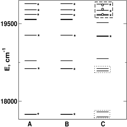
Figure 1: A portion of the energy levels of the model effective Hamiltonian corresponding to polyad $P=6$. The full system is denoted by C and some of the experimental energy levels are shown as open circles. B and A show the energy levels for the subsystems with specific resonances removed. Some of the closely spaced doublets are indicated by $*$. In C the box around the top three levels indicates levels with $4,5$, and $6$ quanta of excitation in the stretch mode.

III Dynamical tunneling: illustration and quantum viewpoint

In the rest of the paper the zeroth-order states will be denoted by $|n_{1}n_{2}\rangle$ since the bend quantum number $n_{b}$ is fixed by the polyad $P$. In order to illustrate the concept of dynamical tunneling we consider zeroth-order degenerate states $|20\rangle$ and $|02\rangle$ with only the 2:1 resonances present i.e., $g^{\prime}=\gamma=0$ in eq. 1. As $\langle 20|\hat{V}^{(1b)}_{2:1}|02\rangle=0=\langle 20|\hat{V}^{(2b)}_{2:1}|02\rangle$ the state $|20\rangle$ has no direct coupling to the symmetric counterpart $|02\rangle$. Nonetheless there is an indirect coupling via the 2:1 resonances. However, as shown in Fig. 2a the zeroth-order state is quite far from the region of state space which can potentially come under the influence of the 2:1 anharmonic resonances. A classical trajectory initiated with initial conditions corresponding to the state $|2,0\rangle$ will continue to stay in that region of the phase space forever without reaching the symmetric region corresponding to the state $|02\rangle$. One such classical trajectory, for about $0.25$ ns, in phase space is shown in Fig. 2b (inset). This classical trapping occurs despite no apparent energetic barriers since in Fig. 2a we show the classical actions satisfying $H_{0}\approx E^{0}_{20}$ which connects the two states. However, contrary to the classical observation, in Fig. 2b the quantum survival probability of the state $|20\rangle$ shows transfer of population to $|02\rangle$ with a period of about $0.20$ ns. In a two-state approximation this corresponds to a splitting of the degenerate levels $\Delta_{2}\approx 0.17$ cm^-1. This is the phenomenon of dynamical tunneling. Previous discussionssihy ; husihy ; stuma2 of dynamical tunneling have used the effective Hamiltonian with only the primary 1:1 present. Here we delibrately show this effect with the 2:1s only to emphasize the role of induced resonances.

A possible explanation of the tunneling arises from the vibrational superexchangehusihy ; stuma2 perspective wherein zeroth-order states coupled locally by the 2:1 perturbations to $|20\rangle$ and $|02\rangle$ are considered. One then constructs all possible perturbative chains connecting the states $|20\rangle$ and $|02\rangle$. An example of such a chain, shown in Fig. 2a, is $|20\rangle\rightarrow|10\rangle\rightarrow|11\rangle\rightarrow|01\rangle\rightarrow|02\rangle$. The contribution to the splitting is

$$\beta^{4}\frac{\langle 20|\hat{V}^{(1b)}|10\rangle\langle 10|\hat{V}^{(2b)}|11\rangle\langle 11|\hat{V}^{(1b)}|01\rangle\langle 01|\hat{V}^{(2b)}|02\rangle}{(\Delta E^{0}_{10})^{2}(\Delta E^{0}_{11})}$$ (5)

with $\Delta E^{0}_{n_{1}n_{2}}\equiv E^{0}_{20}-E^{0}_{n_{1}n_{2}}$. In principle there are an infinite number of chains that connect the two degenerate states. In practice, due to the energy denominators it is sufficient to consider the minimal length chainsself . By minimal length chains one means inclusion of all possible perturbative terms at the lowest order of perturbation necessary. For instance in the example above it is necessary to go to atleast fourth order in perturbation theory, thus scaling like $\beta^{4}$, to get a finite value for the splitting. In our case there are six minimal chains and summing the contributions one obtains a splitting of about $0.18$ cm^-1 which compares well with the exact splitting.

More generally, splitting for any set of degenerate states $|r0\rangle$ and $|0r\rangle$, at minimal order, can be calculated asself :

$$\Delta_{r}=\sum_{abc}\beta^{a}g^{b}\gamma^{c}\sum_{\mu}\Delta_{r}(\Gamma^{(\mu)}_{abc})$$ (6)

with $\mu$ being an index of all possible chains $\Gamma_{abc}$ for a particular choice of $a,b,c$ satisfying the constraint $a+2b+4c=2r$. Indeed such a calculation can be done on our model system and the resulting perturbative estimates are compared to the exact splittings in Fig. 3. For further discussions the superexchange calculations have been compared to the exact results for cases $A,B$, and $C$. At the outset note that the perturbative calculations essentially reproduce, to quantitative accuracy, almost all of the splittings. This degree of accuracy, given high orders of perturbation and number of chains, is pleasantly surprising. For instance the inset to Fig. 3 shows that $130$ contributions of varying signs, some as large as $10^{-4}$, conspire to yield the correct splitting of about $10^{-7}$ for $\Delta_{6}$. Two important observations can be made at this juncture. First, the significant role of the tiny 2:2 resonance is clear in that addition of this 2:2 to the 2:1s enhances the splittings by many orders of magnitude - something which is not readily apparent from Fig. 1. For even values of $r$, especially $r=2$, this is expected since the 2:2 provides a dominant coupling. In fact for $r=2$ one expects $\Delta_{2}\approx 4\gamma=3.6$ cm^-1 which compares very well to the exact value of $3.8$ cm^-1. However, it is significant to note that such a calculation for $r=6$ is too small by a factor of five and that the odd $r$ states would not split at all in the presence of a 2:2 coupling alone. Secondly in all three cases $A,B$, and $C$ the splittings more or less monotonically decrease with increasing stretch excitations. The one exception is in the full system (case $C$) for the state with $r=4$. Later it is shown that this is an instance of suppression of tunneling due to an avoided crossing between the doublet and a third ’intruder’ state. Incidentally in the experimental datatenny pertaining to $r=4$ among the doublets, denoted in the local mode basis as $(40)^{\pm}4$, only the state $(40)^{-}4$ is reportedtenpers . This, given our model Hamiltonian, could be a pure accident!

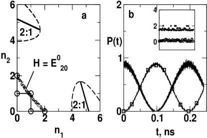
Figure 2: Classical and quantum viewpoints on dynamical tunneling for subsystem $A$. The states are $|02\rangle$ and $|20\rangle$. (a) The state space for polyad $P=6$ is shown with the regions strongly influenced by the 2:1 anharmonic resonances. An example of a minimal (solid) superexchange chain connecting the states is shown. The energy contour satisfying $H_{0}\approx E^{0}_{20}$ is shown connecting the two states. (b) Quantum survival probabilties for $|20\rangle$ and $|02\rangle$ (squares) are shown for $0.25$ ns. Note the almost coherent transfer of population with a period of $0.20$ ns. The inset shows a classical trajectory initiated near $|20\rangle$ for a time period of about $0.25$ ns. The time variations of the actions $(I_{1}-1/2)$ and $(I_{2}-1/2)$ are shown as filled and unfilled circles respectively. The actions stay trapped for the entire period.

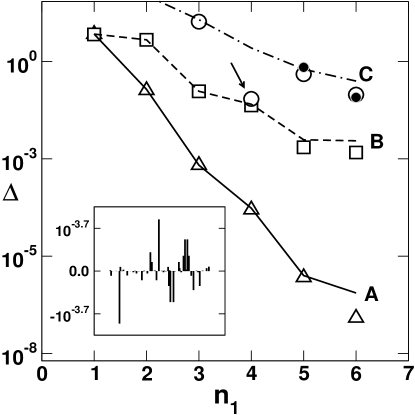
Figure 3: Comparison of the exact quantum (symbols) dynamical tunneling splittings $\Delta$, in cm^-1, to the superexchange results (lines). Shown are the splitting between the states $|n_{1}=r,n_{2}=0\rangle$ and $|0r\rangle$. The $r=1,2$ cases are not shown for the full system since on inclusion of the large 1:1 they are not local modes but resonant normal modes with large splittings. The experimental values for the splitting for $r=5,6$ are shown as filled circles for comparison. The arrow indicates the substantial deviation of the superexchange result from the exact value for $r=4$. The inset shows the contribution from $130$ terms for the superexchange calculation of $\Delta_{6}$ in case A.

It is important to note that the superexchange approach invokes the 2:1 resonant terms without any reference to the classical phase space. This surprisingly good accuracy seems to hold whenever the phase space is integrable or near-integrable and is perhaps related to the equivalence of the superexchange to the WKB approachstuma2 . If this observation is true in multidimensional systems then a phase space perspective on dynamical tunneling should be able to provide some insights. Apart from providing a phase space analog to the superexchange approach it would also be possible to study the extent of sensitvity of dynamical tunneling to the various classical structures. The rest of the paper is dedicated to uncovering precisely such a phase space picture.

IV Dynamical tunneling: phase space viewpoint

IV.1 Induced resonances and dynamical barriers

In what follows, the classical Poincaré surface of sections are plotted in $((I_{1}-I_{2})/2,(\theta_{1}-\theta_{2}))\equiv(K_{1}/2,2\phi_{1})$ at constant values of the sectioning angle $\phi=\theta_{1}+\theta_{2}-4\theta_{b}$ with $\dot{\phi}>0$. In this representation the normal-mode resonant regions appear around $I_{1}\sim I_{2}$. Local modes regions correspond to above and below the normal-mode regions and large 2:1 bend/local-stretch resonant islands appear in the local mode regions.

We begin by asking the question as to what possible structure in the classical phase space is mediating the dynamical tunneling in Fig. 2b. The answer, based on earliersihy ; sibert ; husihy ; stuma2 ; davhel works, should involve a nonlinear resonance zone in the phase space. Indeed the Poincaré surface of section at $E=E^{0}_{20}\approx 18641$ cm^-1 shown in Fig. 4 indicates a resonance zone juxtaposed between the zeroth-order states as seen in the phase space. The surface of section is consistent with the state space view in Fig. 2a in that the primary 2:1 resonances do not appear in the phase space. The 2:1 resonance zones, if present, would show up in Fig. 2a around $K_{1}/2\approx\pm 2.6$. Hence a direct involvement of the 2:1 resonances is ruled out but surely the existence of the 2:1s must be giving rise to a dynamical barrier, in the form of the observed resonance zone, mediating the tunneling. In order to confirm that this nonlinear resonance is mediating the dynamical tuneling it is necessary to extract an explicit expression for the dynamical barrier and obtain the splitting. For this purpose we apply methods of nonlinear dynamicsjoy ; licht on the classical Hamiltonian eq.4 with $g=0=\gamma$ and $\beta\neq 0$. The analysis below is not new and can be found in many of the earlier works including Ozorio de Almeidaozo and Sibertsibert . For completeness sake only essential results are explicitly given and technical aspects of classical perturbation theory will not be discussed.

To start with a canonical transformation is performed $({\bf I},{\bm{\theta}})\rightarrow({\bf J},{\bm{\psi}})$ using the generating function

$$F=(\theta_{1}-2\theta_{b})J_{1}+(\theta_{2}-2\theta_{b})J_{2}+\theta_{b}N$$ (7)

The choice of the generating function implies $\psi_{k}=\theta_{k}-2\theta_{b}$, $J_{k}=I_{k}$ for $k=1,2$ and $\psi_{3}=\theta_{b},N=2(I_{1}+I_{2})+I_{b}$. The resulting Hamiltonian

$$H({\bf J},{\bm{\psi}};N) = H_{0}({\bf J};N)+\epsilon\beta_{c}(N-2J_{1}-2J_{2})$$

$$\times [\sqrt{J_{1}}\cos\psi_{1}+\sqrt{J_{2}}\cos\psi_{2}]$$

is ignorable in the angle $\psi_{3}$ implying the conserved quantity $N=P+5/2$ which is the classical analog of the polyad number $P$. The above two-dimensional Hamiltonian contains the 2:1 resonances and hence nonintegrable. However the phase space from Fig. 4 suggests that at $E\approx E^{0}_{2,0,12}$ the 2:1s do not have a direct role to play. Another way of stating this is that the nonlinear frequencies $\Omega_{k}\equiv\partial H_{0}({\bf I})/\partial I_{k}$ are far away from the condition $\Omega_{1,2}-2\Omega_{b}=0$ for the states in consideration. For the system parameters in this study the $|2,0,8\rangle$ state is detuned by almost $800$ cm^-1. Consequently a formal parameter $\epsilon$ has been introduced with the aim of perturbatively removing the 2:1 resonances, characterized by $\psi_{1,2}$ in eq. IV.1, to $O(\epsilon)$. This can be done by invoking the generating function

$$G=\bar{J}_{1}\psi_{1}+\bar{J}_{2}\psi_{2}+\epsilon[g_{1}\sin\psi_{1}+g_{2}\sin\psi_{2}]$$ (9)

where the functions $g_{1,2}=g_{1,2}(\bar{J}_{1},\bar{J}_{2})$ are determined by the condition of the removal of the primary 2:1s to $O(\epsilon)$. The angles conjugate to ${\bar{\bf J}}$ are denoted by ${\bar{\bm{\psi}}}$. The new variables $({\bar{\bf J}},{\bar{\bm{\psi}}})$ are related to the variables $({\bf J},{\bm{\psi}})$ through the relations $J_{1,2}=\partial G/\partial\psi_{1,2}$ and $\bar{\psi}_{1,2}=\partial G/\partial{\bar{J}}_{1,2}$. Using the identities:

$$\cos(\epsilon z\sin(\varphi)) = {\cal J}_{0}(\epsilon z)+2\sum_{l\geq 1}{\cal J}_{2l}(\epsilon z)\cos(2l\varphi)$$ (10)

$$\sin(\epsilon z\sin(\varphi)) = 2\sum_{l\geq 0}{\cal J}_{2l+1}(\epsilon z)\sin((2l+1)\varphi)$$ (11)

with ${\cal J}_{k}$ being the Bessel functions, it can be shown that

$$H({\bar{\bf J}},{\bar{\bm{\psi}}};N)=\bar{H}_{0}({\bar{\bf J}};N)+\sum_{k}\epsilon^{k}H_{k}({\bar{\bf J}},{\bar{\bm{\psi}}};N)$$ (12)

where

$$\bar{H}_{0}=\Omega_{s}(\bar{J}_{1}+\bar{J}_{2})+\alpha_{ss}(\bar{J}_{1}^{2}+\bar{J}_{2}^{2})+\alpha_{12}\bar{J}_{1}\bar{J}_{2}$$ (13)

with $\Omega_{s}=\omega_{s}-2\omega_{b}+(x_{sb}-4x_{b})N,\alpha_{ss}=x_{s}+4x_{b}-2x_{sb}$ and $\alpha_{12}=8x_{b}-4x_{sb}+x_{ss}$. At $O(\epsilon)$

$$H_{1}({\bar{\bf J}},{\bar{\bm{\psi}}};N)=\sum_{k=1,2}(\beta_{c}\bar{J}_{b}\sqrt{\bar{J}_{k}}+g_{k}({\bar{\bf J}})\widetilde{\Omega}_{k})\cos\bar{\psi}_{k}$$ (14)

where we have denoted $\bar{J}_{b}\equiv N-2(\bar{J}_{1}+\bar{J}_{2})$, and $\widetilde{\Omega}_{k}\equiv\partial\bar{H}_{0}/\partial\bar{J}_{k}$. The action $\bar{J}_{b}$ is essentially the number of bend quanta in the system. The choice of the functions

$$g_{k}({\bar{\bf J}})=-\beta_{c}\frac{\bar{J}_{b}\sqrt{\bar{J}_{k}}}{\widetilde{\Omega}_{k}}$$ (15)

eliminates the 2:1s to $O(\epsilon)$ and hence the $O(\epsilon^{2})$ term in the transformed Hamiltonian eq. 12 is determined to be:

$$H_{2}({\bar{\bf J}},{\bar{\bm{\psi}}};N)=\sum_{k=1,2}\lambda_{k}(1+\cos 2\bar{\psi}_{k})+\lambda_{\pm}\cos(\bar{\psi}_{1}\pm\bar{\psi}_{2})$$ (16)

The term $\cos(\bar{\psi}_{1}-\bar{\psi}_{2})$ is easily identified with a 1:1 resonance between the modes $1$ and $2$ and the strength of this induced 1:1 resonance is obtained as

$$\lambda_{-}({\bar{\bf J}};N)=\frac{1}{2}\beta_{c}^{2}\left[\frac{2(\widetilde{\Omega}_{1}+\widetilde{\Omega}_{2})+\alpha_{12}\bar{J}_{b}}{\widetilde{\Omega}_{1}\widetilde{\Omega}_{2}}\right]\bar{J}_{b}\sqrt{\bar{J}_{1}\bar{J}_{2}}$$ (17)

Expressions for the strengths $\lambda_{1,2}$ and $\lambda_{+}$ are not needed for our analysis hereafter and hence not explicitly given in this work.

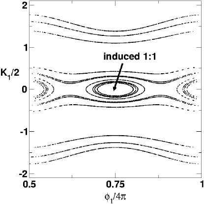
Figure 4: Classical Poincaré surface of section for $H_{A}$ at $E\approx E^{0}_{20}$ showing the induced 1:1 resonance island due to the two stretch-bend 2:1 resonances.

At this stage the transformed Hamiltonian to $O(\epsilon^{2})$ in eq. 16 still depends on both the angles $\bar{\psi}_{1}$ and $\bar{\psi}_{2}$ and hence non-integrable. In order to isolate the induced 1:1 resonance we perform a canonical transformation to the variables $({\bf K},{\bm{\phi}})$ using the generating function $G=(\bar{\psi}_{1}-\bar{\psi}_{2})K_{1}/2+(\bar{\psi}_{1}+\bar{\psi}_{2})K_{2}/2$ and average the resulting Hamiltonian over the fast angle $\phi_{2}$. The resonance center, $K_{1}^{r}=0$, approximation is invoked resulting in a pendulum Hamiltonian describing the induced 1:1 resonance island structure seen in the surface of section shown in Fig. 4. Within the averaged approximation the action $K_{2}=\bar{J}_{1}+\bar{J}_{2}$ is a constant of the motion and can be identified as the 1:1 polyad associated with the secondary resonance. The resulting integrable Hamiltonian is given by

$$\bar{H}(K_{1},\phi_{1};K_{2},N)=\frac{1}{2M_{11}}K_{1}^{2}+2g_{ind}(K_{2},N)\cos 2\phi_{1}$$ (18)

where

$$M_{11} = 2(\alpha_{12}-2\alpha_{ss})^{-1}$$ (19a)

$$g_{ind}(K_{2},N) = \frac{\beta_{c}^{2}}{2}\bar{f}(K_{2},N)(N-2K_{2})K_{2}$$ (19b)

with

$$\bar{f}(K_{2},N)=\frac{4(\Omega_{s}+\alpha_{ss}K_{2})+\alpha_{12}N}{[2(\Omega_{s}+\alpha_{ss}K_{2})+\alpha_{12}K_{2}]^{2}}$$ (19c)

Note, and this is important for the discussion in section IV.2, the averaging procedure does not remove the higher harmonics of the induced 1:1. Thus by focusing on the induced 1:1 alone in eq. 18 we have neglected all induced resonances of the form $q:q$. In terms of the zeroth-order quantum numbers $K_{1}=n_{1}-n_{2}$ and $K_{2}=n_{1}+n_{2}+1\equiv m+1$. Note that eq. 19b, more generally eq. 17, is an analytic expression for the dynamical barrier seperating any two localized states in terms of the zeroth-order actions $(I_{1},I_{2},I_{b})$.

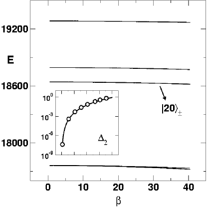
Figure 5: Variation of the $|20\rangle_{\pm}$ doublet energies with the 2:1 resonance strength $\beta$. Results correspond to $H_{A}$ and no exact or avoided crossings are observed. The inset compares the splittings $\Delta_{2}$ calculated semiclassically (open circles, eq. 20) to the exact quantum (solid line) over the same range of $\beta$ variation. Note that $\Delta_{2}$ increases by a factor of $10^{8}$ which is captured well by the induced 1:1 resonance. All quantities are in cm^-1.

One can now use eq. 18 to calculate the dynamical tunneling splitting of the degenerate modes $|n_{1}=r,n_{2}=0,n_{b}=2(P-r)\rangle$ and $|n_{1}=0,n_{2}=r,n_{b}=2(P-r)\rangle$ viastuma2

$$\frac{\Delta^{sc}_{r}}{2} = g_{ind}\prod_{k=-(r-2)}^{(r-2)}\frac{g_{ind}}{E_{R}^{0}(r)-E_{R}^{0}(k)}$$ (20)

$$= g_{ind}\frac{(M_{11}g_{ind})^{r-1}}{2^{r-1}[(r-1)!]^{2}}$$

where $E_{R}^{0}(k)=k^{2}/2M_{11}$ is the zeroth-order energy. For our example with $r=2,m=2$ using the parameters of the Hamiltonian we find $M_{11}\approx 1.32\times 10^{-2}$ and $g_{ind}\approx 3.93$ cm^-1. Within the pendulum approximation the half-width of the resonance zone can be estimated as $2\sqrt{2M_{11}g_{ind}}\approx 0.64$. This estimate, relalizing that $K_{1}\approx(I_{1}-I_{2})$, is in good agreement with the surface of section in Fig. 4. The resulting splitting $\Delta_{2}^{sc}\approx 0.20$ cm^-1 agrees well with the exact splitting. This proves that the induced 1:1 resonance arising from the interaction of the two primary 2:1 resonances is mediating the dynamical tunneling between the degenerate states. Moreover, from a superexchange perspective it is illuminating to note that the splitting can be calculated trivially by recognizing the secondary phase space structure (a viewpoint emphasized in Ref. rat2, as well). This observation emphasizes the superior nature of a phase space viewpoint on dynamical tunneling. The analysis above also sheds light on the relation between the quantum superexchange viewpoint and WKB approximation. Note that $g_{ind}\sim\beta^{2}$ and thus the phase space viewpoint, with $\Delta_{2}\sim g_{ind}^{2}$ is equivalent to the superexchange approach with $\Delta_{2}\sim\beta^{4}$. In this near-integrable situation this correspondence generalizes the observation by Stuchebrukhov and Marcus about the equivalence of superexchange and WKB methods for integrable systemsstuma2 .

IV.2 Higher harmonics and level crossings

In this section we address two issues relevant in the context of dynamical tunneling. The first issue has to do with the role and relation of eigenvalue avoided crossingshel9599 ; ksjpca to nonlinear resonances and hence the phenomenon of dynamical tunneling. Since we have just argued for the involvement of the 2:1 resonances in mediating the dynamical tunneling between degenerate states it is interesting to ask if the states are also involved in an avoided crossing as the 2:1 strength $\beta$ is varied. The answer to this question is negative and Fig. 5 provides evidence that the states $|20\rangle_{\pm}$ do not undergo any identifiable avoided or exact crossings with varying $\beta$. In fact the splittings (Fig. 5 inset) predicted from eq. 20 agree fairly well over the entire range of $\beta$. It is also worthwhile noting that for the system $H_{A}$ the splittings $\Delta_{1,2,3}$ are described quite well by a single induced 1:1 resonance. Therefore, in general, it is not necessary that dynamical tunneling between two zeroth-order states $|n_{1}n_{2}\rangle$ and $|n_{1}+p,n_{2}-q\rangle$ be mediated by a $p:q$ nonlinear resonance alone.

A second issue has to do with the role of higher harmonics or Fourier components in dynamical tunnelinghel9599 . The doublet splitting $\Delta_{2}$ for $H_{A}$ was seen to arise from a induced 1:1 resonance. The perturbative analysis, on the other hand, even in the averaged approximation contains all the higher harmonics of the induced 1:1. These Fourier components appear at higher orders in $\epsilon$ and have very small, but finite, contribution to $\Delta_{2}$. If for some reason the leading order induced 1:1 were to vanish then the higher Fourier components become important. For the present example the 2:2 component would be especially significant. In order to demonstrate this effect consider the Hamiltonian

$$\hat{H}=\hat{H}_{0}-|g|\hat{V}^{(12)}_{1:1}+\beta(\hat{V}^{(1b)}_{2:1}+\hat{V}^{(2b)}_{2:1})$$ (21)

A 1:1 resonance has been added to $H_{A}$ with a strength opposite in sign to the induced 1:1 resonance. The strength $g$ is varied for fixed $\beta$ and there is a specific value of $g=g_{0}$ for which the primary and the induced 1:1 resonance cancel each other out. The value of $g_{0}$ can be estimated by recognizing the integrable pendulum approximation to the above Hamiltonian as

$$\bar{H}\approx\frac{1}{2M_{11}}K_{1}^{2}+(-|g|K_{2}+2g_{ind})\cos 2\phi_{1}$$ (22)

Thus around $|g|_{0}\approx 2g_{ind}/K_{2}$ the above leading order approximation would predict a shutdown of dynamical tunneling. From the estimates provided earlier it is easy to obtain the value $|g|_{0}\approx 2.62$ cm^-1 for $\Delta_{2}$.

In Fig. 6a the variation of the exact splitting $\Delta_{2}$ is shown as a function of $g$. The results clearly show the destruction of tunneling near $g_{0}$ but a more significant observation is that at $g_{0}$, labeled by region ${}^{\prime}M^{\prime}$ in Fig. 6a, the actual value of the splitting is far from zero. This is in contrast to the prediction of shutdown of dynamical tunneling based on the integrable pendulum approximation above. The corresponding phase space in fig. 6M indeed shows that the 1:1 resonance zone has almost vanished. So what is mediating the dynamical tunneling in region $M$? Arguments based on some residual 1:1 coupling are quickly dispelled by noting that the width of the resonance zone in Fig. 6M is nowhere close to the required value. Chances of a strong avoided crossing leading to the enhanced splitting are ruled out by inspecting Fig. 6b. Perhaps there is a broad avoided crossing, as suggested by the exact crossing of the doublets $|20\rangle_{\pm}$ in fig. 6b (inset), leading to the two dips in $\Delta_{2}$ (cf. fig. 6a), with the upper state which happens to be a normal mode state. It is relevant to note that the energy seperation between the doublet and normal mode state is almost equal to the mean level spacing. Moreover a superexchange calculation of $\Delta_{2}$ at $M$ including the required minimal chains (cf. eq. 6) $\Gamma_{400},\Gamma_{020}$, and $\Gamma_{210}$, yields a value $1.70\times 10^{-3}$ cm^-1 which is in excellent agreement with the exact value of $1.65\times 10^{-3}$ cm^-1. All this suggests that in the region $M$ a tiny, but leading order, 2:2 with strength $\gamma=\Delta_{2}/4\approx 4.1\times 10^{-4}$ cm^-1 is mediating the dynamical tunneling. A few important observations provide further support and we briefly outline them. Firstly the splitting in region $M$ are very sensitive to adding a perturbation $\pm\gamma V^{(12)}_{2:2}$ to the Hamiltonian in eq. 21 whereas the regions $L$ and $R$ are far less sensitive as shown in Fig. 6a. Secondly, the classical perturbation analysis carried out to higher orders reveals the emergence of an induced 2:2, scaling as $\beta^{2}g$ at $O(\epsilon^{3})$, with strength comparable to $\gamma$. Indeed the exact $\Delta_{2}$ in region $M$ for different values of $\beta$ scales linearly with $\beta^{2}g$. The superexchange calculation also shows that the contribution from the minimal family $\Gamma_{210}$ i.e., $\beta^{2}g$ nearly, but not exactly, balances the contribution from $\beta^{4}$, and $g^{2}$ families. The analysis here is an example of what Pearman and Gruebelepear call as ’phase cancellation’ effect in perturbative chains. Evidently, the analog of this effect in phase space has to do with the destruction of nonlinear resonances. Although only the $r=2$ case has been shown here, similar effects arise for the higher excitations and can be more complicated to interpret.

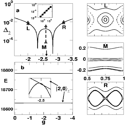
Figure 6: (a) Variation of the exact $\Delta_{2}$ with the primary 1:1 strength $g$. Note the two dips and the relatively flat region denoted by $M$. The arrow indicates the strength $g_{0}$. The effect of adding a small 2:2 with strength $\gamma\approx\pm 4.1\times 10^{-4}$ cm^-1 at specific places are shown as triangles. Inset shows the linear scaling of exact $\Delta_{2}$ (points) with $\beta^{2}|g|_{0}$. In (b) the variation of the relevant energy levels are shown. Inset shows the details for the doublet $|20\rangle_{\pm}$ which undergo two exact crossings. The three panels denoted by $L,M$, and $R$ show the surface of sections corresponding to the regions labeled in (a). The sections are computed using the full classical limit Hamiltonian corresponding to $H_{A}-|g|V_{1:1}^{(12)}$. Note the reorganization of the phase space in going from $L$ to $R$.

IV.3 Multiple resonances: Resonance-assisted tunneling

One of the key lessons learnt from the preceeding discussion is that nonlinear resonances have to be identified in order to obtain a clear phase space picture of dynamical tunneling. Given the near-integrable phase space of $H_{A}$ it is tempting to apply eq. 20 to calculate the splitting of the other doublets corresponding to increasing stretch excitations. In particular the monotonic decrease with increasing stretch excitations, seen in Fig. 3, seems to fit well with the notion of a single resonance (the induced 1:1 here) mediating the tunneling. The naivety of such a viewpoint is illustrated in Fig. 7a. Clearly for $r=1,2,3$ the expectation holds but deviations arise already at $r=4$ and the splittings are many orders of magnitude smaller than the quantum results for $r=5,6$. The reason for this large error is immediately clear from the surface of sections shown in Fig. 7b,c,d. The primary 2:1 resonance has appeared in the phase space and coexists with the induced 1:1. The states corresponding to $r=4,5$ are ’resonant’ local modes and a Husimi representation of the eigenstate in the classical phase space (cf. Fig. 10a) confirms their nature. The $r=5$ doublets are in fact localized in the large 2:1 resonance islands. This can also be anticipated from the state space location of the resonance zones shown in Fig. 2a. Thus a single rotor integrable approximation is insufficient to describe the dynamical tunneling for such cases. Notice the rich structure of the phase spaces in Fig. 7b,c,d resulting from the presence of two ’distant’ and ’nonoverlapping’ (in the Chirikovchiri sense) resonances - a clear manifestation of the nontrivial nature of the near-integrable systems.

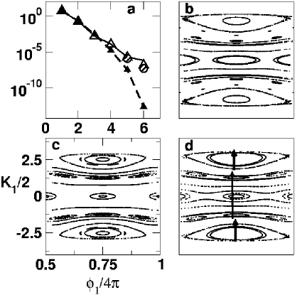
Figure 7: (a) Comparison of the exact (open triangles), superexchange (solid line), and the phase space resonance based (filled triangles) splittings for $H_{A}$ versus excitation quanta in the OH-stretch. Multiple resonance corrections to $r=5,6$ are shown by shaded circles. See text for details. In (b), (c), and (d) the surface of sections at energies corresponding to $r=4,5$, and $6$ respectively are shown. The axes ranges for (b) and (d) are identical to those shown in (c). In (d) one possible dynamical tunneling sequence is shown by arrows.

Is it possible to use the phase space structure, for example in Fig. 7d, and calculate the splitting $\Delta_{6}$? The phase space shows the existence of the primary 2:1s, the induced 1:1, and a thin multimode resonance. For now we will ignore the multimode resonance and consider the primary 2:1s and the induced 1:1 to be independent. This is a strange approximation given that both the induced 1:1 and the multimode arise due to the 2:1s. However, since they are ’isolated’ from each other and lacking any other simple approach we take this viewpoint and compute the splitting. This approach has been advocated earlier by Brodier, Schlagheck and Ullmo in their analysisrat2 of resonance-assisted tunneling in kicked maps. In the present case the effective $\hbar$ is too large to be in the semiclassical limit and hence quantitative accuracies are not expected. At the same time this is a blessing in disguise since we do not have to deal with the the myriad of resonance zones in the phase space! Schematically we imagine the following (cf. Fig. 7d):

$$|60\rangle\stackrel{{\scriptstyle\beta_{eff}}}{{\longrightarrow}}|40\rangle\stackrel{{\scriptstyle g_{ind}}}{{\longrightarrow}}|04\rangle\stackrel{{\scriptstyle\beta_{eff}}}{{\longrightarrow}}|06\rangle$$ (23)

where $\beta_{eff}$ is the effective coupling across the 2:1 islands and $g_{ind}$ is the effective 1:1 coupling derived in the previous section. It is important to note that the $g_{ind}$ value appropriate to $r=6$ needs to be used i.e., the resonance zone width as seen in the surface of section in Fig. 6d. The effective 2:1 couplings can be extracted by approximating the 2:1 resonances, for instance the top island in Fig. 7d, by a pendulum Hamiltonian:

$$\frac{1}{2M_{21}}(J_{1}-J_{1}^{r})^{2}+2\beta_{p}\cos\psi_{1}$$ (24)

with $M_{21}=(2\alpha_{ss})^{-1}$ and $\beta_{p}=\beta_{c}(N-2J_{2}-2J_{1}^{r})\sqrt{J_{1}^{r}}/2$. The resonance center $J_{1}^{r}=-M_{21}(2\Omega_{s}+\alpha_{12})/2\approx 5.7$. The effective coupling is thus estimated as:

$$\beta_{eff}\approx\frac{\beta_{p}^{2}}{E_{6}^{0}-E_{5}^{0}}$$ (25)

with $E_{n}^{0}=(\hbar(n_{1}+1/2)-J_{1}^{r})^{2}/(2M_{21})$. The splitting is then calculated via the expression

$$\Delta_{6}\approx\left(\frac{\beta_{eff}}{E_{6}^{0}-E_{4}^{0}}\right)\times\Delta_{4}^{sc}\times\left(\frac{\beta_{eff}}{E_{6}^{0}-E_{4}^{0}}\right)$$ (26)

where $\Delta_{4}^{sc}$ is the splitting for $r=4$ calculated assuming the induced 1:1 resonance alone. Using the numerical values for the various parameters we find $\Delta_{6}\approx 4.8\times 10^{-8}$ cm^-1 as compared to the exact value of $1.4\times 10^{-7}$ cm^-1. This simple estimate is quite encouraging if one also considers the fact that the induced 1:1 alone would give $\sim 10^{-13}$ cm^-1 and the superexchange value is $6.5\times 10^{-7}$ cm^-1. Similar calculation for $r=5$ doublet also improves the result as shown in Fig. 7a. This simple minded scheme has been tested for other parameters and the results are comparable to the present case. Further support for such an approach comes from considering the $r=6$ doublet splitting with an additonal 2:2 resonance present i.e., described by the Hamiltonian $H_{B}$. From Fig. 3 it is clear that the addition of the 2:2 results in about four orders of magnitude increase in $\Delta_{6}$. The phase space is still near-integrable and a calculation based on the 2:2 alone underestimates the exact result of $3.7\times 10^{-3}$ cm^-1 by nearly a factor of four. Once again employing the approach of hopping across the 2:1 using $\beta_{eff}$, followed by the 2:2 connecting $|40\rangle$ to $|04\rangle$, and hopping across the symmetric 2:1 island improves the result yielding a splitting of about $2.8\times 10^{-3}$ cm^-1. Interestingly the superexchange calculation has a dominant contribution of similar magnitude from the family $\Gamma_{402}$ which is readily identified with the $\beta^{4}\gamma^{2}$ ’path’ in phase space outlined above. The analysis here indicates that it is conceivable that nonlinear resonances can lead to dynamical tunneling between energetically similar regions of phase space even in nonsymmetric situations.

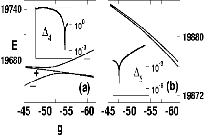
Figure 8: Variation of eigenenergies with the 1:1 strength parameter $g$. (a) $r=4$ doublet involved in an avoided crossing with a $-$ parity normal mode state. Inset shows the behaviour of $\Delta_{4}$ with varying $g$. (b) Same as in (a) for the $r=5$ doublets. All parameters are in cm^-1. Note that the inset x-axis range for $g$ is from $0$ to $-60$ cm^-1. Chaos is visible in the phase space for $|g|>30$ cm^-1.

IV.4 Mixed phase space: Chaos-assisted tunneling?

Up until this point dynamical tunneling was investigated with the underlying phase space being integrable or near-integrable. We now look at the full system $H_{C}$ which exhibits mixed chaotic-regular phase space. The phenomenon of chaos-assisted (suppressed) tunneling (CAT) has to do with the coupling of quantum states, localized on two symmetry-related regular regions of phase space, with one or more ’irregular’ states delocalized over the chaotic seacat . Clearly such processes cannot be understood within a two-state picture and the sensitivity of the nature of the chaotic states to parametric variations is manifested in the splitting fluctutations of the tunneling doublets. It is also reasonable to expect that the effective $\hbar$ in the system needs to be sufficiently small in order for CAT to manifest itself. Perhaps it is useful to note a recent analysismou by Mouchet and Delande wherein they argue that even in cold atom tunneling experiments the effective $\hbar$ is not small enough to observe CAT. The system investigated herein is nowhere close to such limits and at the outset we do not expect to see CAT. In other words for our full system described by $H_{C}$ only resonance-assisted tunneling (RAT) mechanisms should be sufficient to explain the relevant splittingsmou .

We focus on the doublets $r=4,5,6$ since the phase space shows substantial chaos at the corresponding energies. In Fig. 3 it is seen that the $r=4$ case showed marked deviations from monotonicity. Moreover the superexchange calculation predicted a much higher $\Delta_{4}$. In Fig. 8a we show the variation of energy levels with the 1:1 strength $g$ and a clear avoided crossing between one of the tunnel doublets (with $-$ parity) and a normal mode state is observed. The inset in Fig. 8a implicates the avoided crossing in the observed exact crossing between the tunnel doublets themselves leading to the suppression of tunneling. In Fig. 9 the phase space Husimihusimi representations (refer to ksjcp, for details regarding the computation of the Husimi distributions) of the three states are shown with the corresponding phase space. Notice that the normal mode (’intruder’) state has a much more regular Husimi in the phase space as compared to the doublet Husimis themselves. In particular the $-$ doublet is extensively delocalized over the phase space. Given the value of the effective $\hbar$ it is not possible to declare the $-$ parity doublet to be a chaotic state. Note however that the doublets corresponding to $r=4$ are essentially living in the chaotic regions. For the near-integrable subsystems $H_{A}$ and $H_{B}$ the $r=4$ doublets live on the separatrix associated with the 2:1 resonance. So this is an instance where a regular intruder state is affecting the tunneling between irregular doublets. No attempt is made here to calculate the tunneling splitting semiclassically. However we note that the exact value $\Delta_{4}\approx 0.1$ cm^-1 as compared to the superexchange value of $2.3$ cm^-1. Interestingly with further increase of $g$, resulting in more chaos, the superexchange calculation is only a factor of two higher than the exact value.

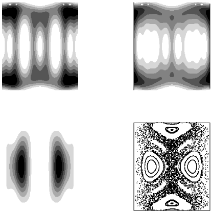
Figure 9: Husimi distributions of the $r=4$ doublets and a close lying normal mode state for the full system $H_{C}$. The axes ranges are identical to those shown in fig. 7b. The dark regions correspond to large values while the light regions signify smaller values. The top row shows the Husimis for the $-$ and $+$ parity states while the bottom left is for the $-$ parity normal mode state. The bottom right panel shows the phase space with clearly identified 1:1 and 2:1 resonance islands. Note the delocalized Husimis of the doublets in contrast to that of the normal mode state.

On the other hand in Fig. 8b the variation of the $r=5$ doublet energies are shown as a function of the 1:1 parameter $g$. This case does not show any avoided crossing. The Husimis for this doublet corresponding to the systems $H_{A},H_{B}$ (near-integrable) and $H_{C}$ (mixed) are shown in Fig. 10a,b, and c respectively. It is notable that the splitting in going from $H_{A}$ to $H_{B}$ increases by more than three orders of magnitude (cf. Fig. 3). The Husimis and surface of sections in Fig. 10a,b are quite similar except for the 2:2 resonance zone clearly visible in Fig. 10b. However, the 2:2 alone cannot mediate dynamical tunneling between the localized states in the 2:1 zone. As in the previous section, excitation out to the seperatrix state $|40\rangle$ followed by tunneling across the 2:2 zone to $|04\rangle$ and finally coupling to the symmetric $|05\rangle$ state captures quantitatively the tunneling enhancement. This is a clear manifestation of RAT in the system. Adding the primary 1:1 resonance, resulting in $H_{C}$, the doublet splitting is further enhanced by two orders of magnitude (cf.Fig. 3). The phase space as shown in Fig. 10 is clearly of a mixed nature. The large 1:1 resonance zones are visible and tentatively one assigns the enhancement in splitting to the 1:1 coupling. The 1:1 alone can account for one order of magnitude enhancement. However of all the possible resonant subsystems considered, quantum mechanically or semiclassically, the best estimate is a factor of two too small as compared to the $\Delta_{5}$ for the full system. In this context an inspection of Fig. 10 Husimi for the full case reveals amplitude spreading through the classically chaotic region. This is in stark contrast to the well localized Husimis in the near-integrable cases. Again the effective $\hbar$ is too large to implicate the classical stochasticity for part of the enhancement in $\Delta_{5}$. Although the case for $r=6$ is not shown here $\Delta_{6}$ is enhanced (cf. fig. 3) by four orders of magnitude in going from $H_{A}$ to $H_{B}$. This enhancement could again be captured quantitatively by the semiclassical analysis. However the best integrable estimate based on the 1:1 and the 2:2 resonances is almost an order of magnitude too small for the full system $H_{C}$.

The upshot of the precceding analysis is that no integrable subsystem can account for the splittings of $H_{C}$ and one atleast needs some chaos to be present. Even subsystems with chaos, for instance 2:1s $+$ 1:1, on exact diagonalization yield splttings which are about a factor of two in error. This points to a fairly subtle involvement by all the resonances, irrespective of their strengths, and is not understood well at this point of time. Reducing the effective $\hbar$ in the system is a theoretical tool to clarify the picture. For our system, a nonscaling one, it is not very easy to perform $\hbar$-scaling computations. Nevertheless some preliminary calculations indicate that the near-integrable cases show exponential fall off with $\hbar^{-1}$ whereas the mixed cases exhibit fluctuations. In particular the $r=4$ doublet splitting exhibits an algebraic dependence $\hbar^{-\alpha}$ rather than the usual $\exp(-1/\hbar)$ dependence.

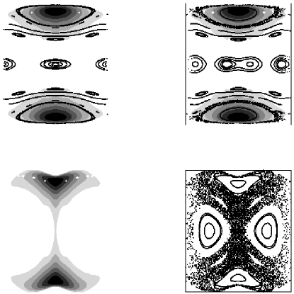
Figure 10: The top panels show the Husimis superposed on phase space for the $+$ symmetric partner of the $r=5$ doublet in the near integrable cases. The axes ranges are identical to those shown in fig. 7c. Top left is for $H_{A}$ (2:1 only) and top right is for $H_{B}=H_{A}+2:2$. The Husimis in both instances are localized in the 2:1 islands. The bottom left panel shows the Husimi for the full case $H_{C}$ and the corresponding phase space is shown in the bottom right. Note the small isthumus across the chaotic sea connecting the two islands.

V Conclusions

In this work an intimate connection between dynamical tunneling and the resonance structure of the classical phase space is established. The order and widths of the resonances determine the explicit dynamical barriers in the zeroth-order action (quantum number) space. The current study indicates that it is safer to ’blame’ dynamical tunneling on the nonlinear resonances without invoking further connections between avoided crossings and the resonances. If accidental avoided crossings occur, as they do in near-integrable, mixed and chaotic systems, then dynamical tunneling can be enhanced or suppressed further. This study also lends support to earlier suggestionshel9599 that even very small resonant couplings can be the cause of the experimentally observed narrow spectral clusters. The resonances responsible for such spectral clusters can be primary or induced resonances and with small but significant amount of stochasticity in the phase space the consequences for energy flow can be nontrivial.

In near-integrable situations, generic to lower energy regimes in large molecules, a combination of more than one resonance zone can control dynamical tunneling. Not only is it important to identify the relevant resonance zones but it is also necessary to prescribe a route to calculate the splittings. It is significant to note that neither of these problems are easy to solve. Again, and not surprisingly, the lack of understanding of the structure of multidimensional phase space is the main bottleneck. In this regard the superexchange approach works well but such an accuracy for high dimensional systems, with mixed regular-chaotic phase spaces, is not guaranteed. As shown in the present work and in a previous workself the superexchange approach is prone to errors, atleast by an order of magnitude, whenever states are involved in avoided crossings. It remains to be seen if going beyond the minimal paths prescription, with some clever ’resummation’ tricks, would lead to quantitative improvements. We have shown that treating the resonance zones as pendulums and coupling across them to connect the two nearly degenerate states provides an approximate route to calculating the tunnel splittings. This chain of resonance zones, in some sense, provides a semiclassical basis for the success of the vibrational superexchange approach. The current work has shown the close correspondence between various terms contributing in the superexchange approach and the underlying resonances in the phase space. The superexchange mechanism itself has its roots in the field of electron transfer in molecular systemsnitz . In this context it is interesting to note the analogy between the role played by the ’bridge’ states connecting the donor and acceptor sites for electron transfernitz and the resonance zones connecting two symmetry related, distant states localized in phase space. Some similarities, perhaps formal, to this work showing the promotion of dynamical tunneling by multiple resonances and a recent workuri demonstrating promotion of deep tunneling through molecular barriers by electron-nuclear coupling further exemplify the close parallels between the phenomena of off-resonant electron transfer and dynamical tunneling. Regarding the various mechanisms of dynamical tunneling in molecules this work suggests that for small molecules with low density of states (large effective $\hbar$) the dominant mechanism would be resonance-assisted. For molecules with sufficiently high density of states (sufficiently small effective $\hbar$) both chaos and resonances can mediate dynamical tunneling and the dominant mechanism is decided by the energy of the doublets and the location of the doublets in the corresponding phase space.

Although the analysis was on coupled three-mode systems the conclusion remains valid in general for systems which exhibit local mode behaviour. This is based on our analysis, along similar lines, for many other systems which are described more naturally by local (D₂O, H₂S) or normal mode (SO₂) limits. For systems with small or vanishing anharmonicities, where the issue of the existence of localized modes itself is moot, the various resonances are still important but any calculation based on a pendulum approximation is clearly invalid. Thus spectra of molecules involving light atom stretch-bend modes are good candidates to observe the fingerprints of dynamical tunneling. In particular we suggest the high overtone spectral regions of the water molecule as one possibility. This suggestion is tentative since a model Hamiltonian has been utilized for the analysis and it is probable that the polyad picture will break down at such high energies. One possibility is to do a detailed analysis on the best potential energy surface available and/or explicitly break the polyad by adding further weak resonances. Both approaches result in genuine three degree of freedom phase spaces and thus a straightforward extension is not easy. Apart from the limitation in visualizing the global phase space structures this has to do with the fact that there are classical phenomenalicht in three or more degrees of freedom that could modify certain aspects of the lower dimensional analysis. For instance in three or higher degree of freedom systems two long time phenomena are controlled by nonlinear resonances - Arnol’d diffusionlicht ; commardif and dynamical tunneling. Precious little is known about either of these phenomena and their possible spectral manifestations in such situations and needs further studycompet . As a final note we comment on the possibility of observing long lived local excitations in systems with multiple resonances. This work shows that additional resonances can modify the near-degeneracies via CAT and RAT. But this modification, by the same additional resonances and resulting chaos, can go either way due to multistate interactions! Moreover, as shown in this work, additional resonances and presumably coupling to rotationslehkk ; orti can also conspire to increase the degeneracy. Coherent manipulation of tunneling using external fields has been demonstrated beforemfield ; cohdesfield and there are reasons to think that such ideas can be utilized in the present context as well.

VI Acknowledgements

It is a pleasure to thank Peter Schlagheck for critical and illuminating discussions. I am grateful to Prof. Klaus Richter for the hospitality and support at the Universität Regensburg where part of this work was done.

References

- (1) M. Quack, Annu. Rev. Phys. Chem. 41, 839 (1990); T. Uzer, Phys. Rep. 199, 73 (1991); K. K. Lehmann et.al., Annu. Rev. Phys. Chem. 45, 241 (1994); D. J. Nesbitt and R. W. Field, J. Phys. Chem. 100, 12735 (1996); M. Gruebele and R. Bigwood, Int. Rev. Phys. Chem. 17, 91 (1998); J. C. Keske and B. H. Pate, Annu. Rev. Phys. Chem. 51, 323 (2000).
- (2) M. E. Kellman, Adv. Chem. Phys. 101, 590 (1997); G. S. Ezra, Adv. Class. Traj. Meth. 3, 35 (1998); M. V. Kuzmin and A. A. Stuchebrukhov, in Laser Spectroscopy of Highly Vibrationally Excited Molecules, Ed. V. S. Letokhov, p. 178 Adam Hilger, Bristol, 1989; A. A. Ovchinnikov, N. S. Erikhman, and K. A. Pronin, Vibrational-Rotational Excitations in Nonlinear Molecular Systems, Kluwer Academic/Plenum, New York, 2001.
- (3) M. J. Davis and E. J. Heller, J. Chem. Phys. 75, 246 (1981);E. J. Heller and M. J. Davis, J. Phys. Chem. 85, 307 (1981). The notion of associating a generalized tunneling with any classically forbidden dynamical event is already found in W. H. Miller, Adv. Chem. Phys. 25, 69 (1974).
- (4) For recent reviews on the local modes see, B. R. Henry and H. G. Kjaergaard, Can. J. Chem. 80, 1635 (2002); P. Jensen, Mol. Phys. 98, 1253 (2000); L. Halonen, Adv. Chem. Phys. 104, 41 (1998).
- (5) C. Jaffé and P. Brumer, J. Chem. Phys. 73, 5646 (1980).
- (6) M. E. Kellman, J. Chem. Phys. 83, 3843 (1985).
- (7) M. Quack, Faraday Discuss. Chem. Soc. 71, 359 (1981).
- (8) S. Flach and C. R. Willis, Phys. Rep. 295, 181 (1998); J. Dorignac and S. Flach, Phys. Rev.B 65, 214305 (2002); S. Flach and V. Fleurov, J. Phys.:Condens. Matter 9, 7039 (1997); V. Fleurov, Chaos 13, 676 (2003) and references therein.
- (9) R. T. Lawton and M. S. Child, Mol. Phys. 37, 1799 (1979); R. T. Lawton and M. S. Child, Chem. Phys. Lett. 87, 217 (1982).
- (10) E. R. Th. Kerstel et. al., J. Phys. Chem. 95, 8282 (1991).
- (11) A. A. Stuchebrukhov and R. A. Marcus, J. Chem. Phys. 98, 6044 (1993).
- (12) A. McIlroy and D. J. Nesbitt, J. Chem. Phys. 91, 104 (1989).
- (13) A. Callegari et. al., Mol. Phys. 101, 551 (2002).
- (14) A. Portnov, S. Rosenwaks, and I. Bar, J. Chem. Phys. 121, 5860 (2004).
- (15) T. K. Minton, H. L. Kim, S. A. Reid, and J. D. McDonald, J. Chem. Phys. 89, 6550 (1988).
- (16) M. E. Kellman, J. Chem. Phys. 76, 4528 (1982).
- (17) W. G. Harter and C. W. Patterson, J. Chem. Phys. 80, 4241 (1984).
- (18) K. K. Lehmann, J. Chem. Phys. 95, 2361 (1991); K. K. Lehmann, J. Chem. Phys. 96, 7402 (1992); See also, M. S. Child and Q. Zhu, Chem. Phys. Lett. 184, 41 (1991).
- (19) R. M. Lees, Phys. Rev. Lett. 75, 3645 (1995); J. Ortigoso, Phys. Rev. A 54, R2521 (1996).
- (20) A. M. Ozorio de Almeida, J. Phys. Chem. 88, 6139 (1984).
- (21) E. L. Sibert III, W. P. Reinhardt, and J. T. Hynes, J. Chem. Phys. 77, 3583, 3595 (1982.
- (22) J. S. Hutchinson, E. L. Sibert III, and J. T. Hynes, J. Chem. Phys. 81, 1314 (1984).
- (23) E. L. Sibert III, J. Chem. Phys. 83, 5092 (1985).
- (24) A. A. Stuchebrukhov and R. A. Marcus, J. Chem. Phys.98, 8443 (1993).
- (25) E. J. Heller, J. Phys. Chem. 99, 2625 (1995); E. J. Heller, J. Phys. Chem. A 103, 10433 (1999).
- (26) R. Roncaglia, L. Bonci, F. M. Izrailev, B. J. West, and P. Grigolini, Phys. Rev. Lett. 73, 802 (1994); L. Bonci, A. Farusi, P. Grigolini, and R. Roncaglia, Phys. Rev. E 58, 5689 (1998).
- (27) O. Brodier, P. Schlagheck, and D. Ullmo, Phys. Rev. Lett. 87, 064101 (2001); O. Brodier, P. Schlagheck, and D. Ullmo, Ann. Phys. 300, 88 (2002).
- (28) O. Bohigas, S. Tomsovic, and D. Ullmo, Phys. Rep. 223, 43 (1993); Tunneling in Complex Systems, edited by S. Tomsovic (World Scientific, Singapore, 1998) and references therein; A. Shudo and K. S. Ikeda, Phys. Rev. Lett. 76, 4151 (1996); S. C. Creagh and N. D. Whelan, Phys. Rev. Lett. 77, 4975 (1996); E. Doron and S. D. Frischat, Phys. Rev. Lett. 75, 3661 (1995); S. D. Frischat and E. Doron, Phys. Rev. E 57, 1421 (1998); J. Zakrzewski, D. Delande, and A. Buchleitner, Phys. Rev. E 57, 1458 (1998).
- (29) C. Eltschka and P. Schlagheck, Phys. Rev. Lett. 94, 014101 (2005).
- (30) J. U. Nöckel and A. D. Stone, Nature 385, 45 (1997); W. K. Hensinger et. al., Nature 412, 52 (2001); D. A. Steck, W. H. Oskay, and M. G. Raizen, Science 293, 274 (2001); A. P. S. de Moura et. al., Phys. Rev. Lett. 88, 236804 (2002).
- (31) W. A. Lin and L. E. Ballentine, Phys. Rev. Lett. 65, 2927 (1990); R. Utermann, T. Dittrich, and P. Hänggi, Phys. Rev. E 49, 273 (1994); D. Farrelly and J. A. Milligan, Phys. Rev. E 47, R2225 (1993); H. P. Breuer and M. Holthaus, J. Phys. Chem. 97, 12634 (1993); M. Gruebele, J. Phys. Condens. Matter 16, R1057 (2004).
- (32) J. E. Baggot, Mol. Phys. 65, 739 (1988).
- (33) S. Keshavamurthy and G. S. Ezra, J. Chem. Phys. 107, 156 (1997); S. Keshavamurthy and G. S. Ezra, Chem. Phys. Lett. 259, 81 (1995).
- (34) M. Joyeux, J. Chem. Phys. 109, 2111 (1998); M. Joyeux and D. Sugny, Can. J. Phys. 80, 1459 (2002).
- (35) M. Joyeux, S. C. Farantos, and R. Schinke, J. Phys. Chem. A 106, 5407 (2002); M. P. Jacobson and R. W. Field, J. Phys. Chem. A 104, 3073 (2000); H. Ishikawa, R. W. Field, S. C. Farantos, M. Joyeux, J. Koput, C. Beck, and R. Schinke, Annu. Rev. Phys. Chem. 50, 443 (1999).
- (36) Z. M. Lu and M. E. Kellman, J. Chem. Phys. 107, 1 (1997).
- (37) J. Tennyson, N. F. Zobov, R. Williamson, O. L. Polyansky, and P. F. Bernath, J. Phys. Chem. Ref. Data 30, 735 (2001).
- (38) A. Bykov, O. Naumenko, L. Sinista, B. Voronin, J.-M. Flaud, C. Camy-Peyret, and R. Lanquetin, J. Mol. Spec. 205, 1 (2001).
- (39) S. Keshavamurthy, J. Chem. Phys. 119, 161 (2003).
- (40) The experimental value for the splitting of the pair is about cm-1. J. Tennyson, personal communication.
- (41) A. J. Lichtenberg and M. A. Lieberman, Regular and Chaotic Dynamics, Springer-Verlag, New York, 1992.
- (42) See, S. Keshavamurthy, J. Phys. Chem. A 105, 2668 (2001) for detailed references and one possible signature of nonlinear resonances in parametric eigenvalue variations.
- (43) R. Pearman and M. Gruebele, J. Chem. Phys. 108, 6561 (1998).
- (44) B. V. Chirikov, Phys. Rep. 52, 263 (1979).
- (45) A. Mouchet and D. Delande, Phys. Rev. E 67, 046216 (2003).
- (46) K. Husimi, Proc. Phys. Math. Soc. Japan 22, 264 (1940).
- (47) See for example, A. Nitzan, Annu. Rev. Phys. Chem. 52, 681 (2001) and references therein.
- (48) M. Abu-Hilu and U. Peskin, J. Chem. Phys. 122, 021103 (2005) and references therein.
- (49) We note that it is perhaps better to think of Arnol’d diffusion in a slightly nonrestrictive sense then that implied by Arnol’d in his seminal work, V. I. Arnol’d, Sov. Math.-Dokl. 5, 581 (1964). For critical reviews see: P. M. Cincotta, New Astr. Rev. 46, 13 (2002); P. Lochak in Hamiltonian Systems with Three or More Degrees of Freedom, Ed. C. Simó, NATO ASI, Kluwer, Dordrecht, pp. 168, 1999; F. Vivaldi, Rev. Mod. Phys. 56, 737 (1984); G. Haller, Phys. Lett. A 200, 34 (1995).
- (50) D. M. Leitner and P. G. Wolynes, Phys. Rev. Lett. 76, 216 (1996); D. M. Leitner and P. G. Wolynes, Phys. Rev. Lett. 79, 55 (1997); E. Tannenbaum, Ph.D. thesis, chapter 3, Harvard University, 2002.
- (51) F. Grossmann, T. Dittrich, P. Jung, and P. Hänggi, Phys. Rev. Lett. 67, 516 (1991); J. Gong and P. Brumer, Annu. Rev. Phys. Chem. 56, advanced article, 2005.