Orbit Determination
with Topocentric Correction:
Algorithms for the Next Generation Surveys

ABSTRACT

Given a set of astrometric observations assumed to belong to the same object, the problem of orbit determination is to compute the orbit with all the necessary tools to assess its uncertainty and reliability. Under the conditions of the next generation surveys, with much larger number density of observed objects, new algorithms, or at least substantial revisions of the classical ones, are needed. The problem has three main steps, preliminary orbit, least squares orbit, and quality control. The classical theory of preliminary orbit algorithms was incomplete, in that the consequences of the topocentric correction had not been fully studied. We show that it is possible to rigorously account for the topocentric correction, possibly with an increase in the number of alternate preliminary orbit solutions, without impairing the overall orbit determination performance. We have developed modified least squares orbit determination algorithms, including fitting methods with a reduced number of parameters (required when the observed arcs have small curvature), that can be used to improve the reliability of the orbit computing procedure. This requires suitable control logic to pipeline the different algorithms which we have defined and validated through numerical simulations. We have tested the complete procedure on two simulations with number densities comparable to that expected from the next generation all-sky surveys such as Pan-STARRS and LSST. To control the problem of false identification (where observations of different objects are incorrectly linked together) we have introduced a quality control on the fit residuals based upon an array of metrics and a procedure of normalization to remove duplications and contradictions in the output. The results confirm that large sets of discoveries can be obtained with good quality orbits and very high success rate losing only $0.6$ to $1.3\%$ of objects and a false identification rate in the range $0.02$ to $0.06\%$.

Key Words: Celestial Mechanics; Asteroids, Dynamics; Orbits

1 The Problem

The problem of preliminary orbit determination is old, with very effective solutions developed by [Laplace 1780] and [Gauss 1809]. Of course the methods of observing Solar System bodies have changed radically since classical times and have been changing even faster recently due to advances in digital astrometry. The question is, what needs to be improved in the classical algorithms to handle the expected rate of data from the next generation of all-sky surveys? Alternatively, what can we now use in place of the classical algorithms?

The issue is not one of computational resources because these grow at the same rate as the capability of generating astrometric data. Reliability is the main problem when handling large astronomical data sets (millions of individual detections of Solar System objects). An algorithm failing once when used $1,000$ times may have been considered perfectly reliable only a few years ago but in the present situation we must demand better performance, and even more so in the near future.

This is particularly important because of the strong correlation between difficulties in the orbit computation and the scientific value of the discovered object. Main Belt Asteroids (MBA) are commonplace and their orbits are easily computed. Only a few in a $1,000$ of the objects (to a given limiting magnitude) are the more interesting Near Earth Objects (NEO) while few in $100$ are the equally interesting Trans Neptunian Objects (TNO); in both cases the computation may be much more difficult for reasons explained later. Thus an algorithm computing orbits for $99\%$ of the discoveries may be failing on a large fraction of the more interesting objects like the NEO and TNOs.

To find reliable algorithms we need a good qualitative understanding of the solutions and a firm control of the approximations used. The classical algorithms contain several approximations, we will show that one of them is the most dangerous: neglecting the topocentric correction and assuming that the observer sits at the center of mass of the Earth. The well known method of reducing to the geocenter by assuming the object’s distance and then iterating the preliminary orbit computation does not solve the problem.

Although Laplace’s and Gauss’ methods each have their supporters it is generally believed that they are equivalent to a good approximation. In fact, we show that this is true only when the topocentric correction is neglected. As already pointed out by [Marsden 1985], Gauss’ method has significant advantages in the way it can include the topocentric correction. However, the classical qualitative theory [Charlier 1910] of the number of alternate solutions for the preliminary orbit applies only to Laplace’s method neglecting the topocentric correction.

We show that a reliable method, effective under the present observing conditions, can account for the topocentric correction in Gauss’ method although such a correction could also be included in Laplace’s method. Then we need a qualitative theory, replacing the one of Charlier, for Gauss’ method that does not assume geocentric observations. We have developed such a theory and found that the number of alternate preliminary orbit solutions can be larger than in Charlier’s theory, namely, there may be double solutions at opposition and triple solutions at low solar elongations.

A reliable orbit determination algorithm should begin with a preliminary orbit algorithm that accounts for the possibility of double and even triple solutions. This is especially important to reliably handle NEO discoveries which are affected by non-unique solutions (occurring in most cases near quadrature and sometimes even at opposition). Moreover, particular provisions are required for the case in which the quantities used as input to the preliminary orbits, the curvature components, are poorly determined to the point that their sign is uncertain. This happens when the observed arc is too short and when the observed object is very distant. For the case in which TNOs are being discovered, weakly determined or totally undetermined preliminary orbits are the rule. Two classes of methods can be used in such cases: the Virtual Asteroids (VA) methods and the constrained least squares solutions.

A Virtual Asteroid is a fully specified orbit with six orbital elements that is compatible with the available observations but by no means determined by them. In different types of VA methods one to thousands (depending upon the purpose) of VA are selected either at random or by some geometric construction inside the region in the space of the orbits compatible with the observations. There are more than half a dozen VA methods available in the literature and we will not review all of them but just present one version which is particularly effective for the problem we are discussing in this paper. It consists in choosing just one VA in such a way that both the condition of being compatible with the observations and having an elliptic orbit are satisfied. It is derived from the theory of the Admissible Region we have developed [Milani et al. 2004]. This is especially effective when the preliminary orbits computed with the classical algorithms (or even modern versions) are ineffective as happens in most cases for TNOs observed near quadrature.

The main purpose of preliminary orbits is to be used as a first guess for the nonlinear optimization procedure (Differential Corrections) that identifies the nominal orbit fulfilling the principle of Least Squares (of the residuals). If the preliminary orbits are well defined by the curvature of the observed path, then one of them is likely to be close enough to some least squares orbit to belong to the convergence domain of the differential corrections; then it is sufficient to use all the preliminary orbits as first guesses. If the preliminary orbits are poorly defined they are likely to be so “wrong” that they will not lead to convergence of the differential corrections, an inherently unstable procedure when using a starting point far from the nominal.

Thus it is essential to increase the size of the convergence domain by using modified differential corrections methods. Many of these methods exist and most of them have one feature in common: the number of parameters determined is less than 6. There are 4-fit methods in which 2 variables are kept fixed (at the value determined by the preliminary orbit or by some other criterion) and the others are corrected in an iteration converging to the minimum of the sum of squares of the residuals restricted to a 4-dimensional submanifold of the 6-dimensional space. There are 5-fit methods in which one parameter is fixed although it does not need to be one of the orbital elements but might be defined in some intrinsic way adapted to the particular problem at hand. The 5-fit method we use is fully documented in [Milani et al. 2005a].

Although the focus of this paper is on new theory and on algorithm documentation we felt the need to thoroughly test the actual performance when our methods and software are confronted with the expected data rate of the next generation surveys. Thanks to the collaboration with the Pan-STARRS [Jedicke et al. 2007] and LSST [Ivezić et al. 2007] projects we have had the opportunity to use simulations of future survey observations to precisely measure performances using the simulation source catalog as ground truth. In particular we report here on two tests, one based on a small but focused simulation containing only the most difficult orbits (NEOs and TNOs), and one representing the full data rate from a next generation survey containing all classes of solar system objects (of course the numbers are dominated by MBA). We believe the results are a convincing confirmation that we are ready to handle the data from the next generation surveys.

2 Equations from the Classical Theory

There are so many different versions of preliminary orbit determination methods and there is so little in the way of a standard notation that it is not possible to simply copy the equations from some reference. Thus, we have chosen to provide here a compact summary of the basic formulae, in particular discussing the dynamical equation and the associated polynomial equation of degree 8 for both methods developed by Gauss and Laplace. We also summarize Charlier’s theory on the number of solutions for Laplace’s method, to be compared to the new qualitative theory, including topocentric correction, of Section 4.

2.1 Laplace’s Method

The observation defines the unit vector $\hat{\bm{\rho}}=(\cos{\delta}\cos{\alpha},\cos{\delta}\sin{\alpha},\sin{\delta})$ where $(\alpha,\delta)$ are the topocentric right ascension and declination. The heliocentric position of the observed body is

$$\mathbf{r}=\bm{\rho}+\mathbf{q}=\rho\hat{\bm{\rho}}+q\hat{\mathbf{q}}$$

where $\mathbf{q}$ is the observer’s position. Let $s$ be the arc length parameter for the path described by the relative position $\hat{\bm{\rho}}(t)$ and $\eta$ the proper motion

$$\frac{ds}{dt}=\eta=\sqrt{\dot{\alpha}^{2}\cos^{2}{\delta}+\dot{\delta}^{2}}\ ;\ \frac{d}{ds}=\frac{1}{\eta}\frac{d}{dt}\ .$$

We use the moving orthonormal frame [Danby 1962, Sec. 7.1]

$$\hat{\bm{\rho}}\ ,\ \hat{\mathbf{v}}=\frac{d\hat{\bm{\rho}}}{ds}\ ,\ \hat{\mathbf{n}}=\hat{\bm{\rho}}\times\hat{\mathbf{v}}$$ (1)

and define the geodesic curvature $\kappa$ by the equation

$$\frac{d\hat{\mathbf{v}}}{ds}=-\hat{\bm{\rho}}+\kappa\hat{\mathbf{n}}\ .$$ (2)

Then the relative acceleration is

$$\frac{d^{2}\bm{\rho}}{dt^{2}}=(\ddot{\rho}-\rho\eta^{2})\hat{\bm{\rho}}+(\rho\dot{\eta}+2\dot{\rho}\eta)\hat{\mathbf{v}}+(\rho\eta^{2}\kappa)\hat{\mathbf{n}}$$ (3)

and the differential equations of relative motions are

$$\frac{d^{2}\bm{\rho}}{dt^{2}}=\ddot{\mathbf{r}}-\ddot{\mathbf{q}}=\frac{\mu\mathbf{q}}{q^{3}}-\frac{\mu\mathbf{r}}{r^{3}}$$ (4)

with the following approximations: $\mathbf{q}=\mathbf{q}_{\oplus}$ coincides with the center of mass of the Earth, the only force operating on both the Earth and the object at $\mathbf{r}$ is the gravitational attraction by the Sun, i.e. there are no planetary perturbations (not even indirect perturbation by the Earth itself). From (3)$\cdot\hat{\mathbf{n}}=$(4)$\cdot\hat{\mathbf{n}}$

$$\frac{d^{2}\bm{\rho}}{dt^{2}}\cdot\hat{\mathbf{n}}=\rho\eta^{2}\kappa=\mu\;q\;\hat{\mathbf{q}}\cdot\hat{\mathbf{n}}\left(\frac{1}{q^{3}}-\frac{1}{r^{3}}\right)\ ,$$

which can be presented in the form

$$C\frac{\rho}{q}=1-\frac{q^{3}}{r^{3}}\ \ \mbox{with}\ \ C=\frac{\eta^{2}\kappa q^{3}}{\mu\hat{\mathbf{q}}\cdot\hat{\mathbf{n}}}$$ (5)

referred to as the dynamical equation in the literature on preliminary orbits. $C$ is a non-dimensional quantity that can be $0$ when $r=q$ or undetermined (of the form ${0}/{0}$) in the case that the $O(\Delta t^{2})$ approximation fails, i.e. the object is on an inflection point with tangent pointing to the Sun.

Given $\rho$, to complete the initial conditions $\dot{\rho}$ is solved from (3)$\cdot\hat{\mathbf{v}}=$(4)$\cdot\hat{\mathbf{v}}$

$$-\mu\frac{\bm{q}\cdot\hat{\mathbf{v}}}{r^{3}}+\mu\frac{\bm{q}\cdot\hat{\mathbf{v}}}{q^{3}}=\rho\dot{\eta}+2\dot{\rho}\eta\ .$$ (6)

2.2 Charlier’s Theory

Eq. (5) is the basic formula for Laplace’s method using the solution in terms of either $\rho$ or $r$ which are not independent quantities. From the triangle formed by the vectors $\mathbf{q},\bm{\rho},\mathbf{r}$ we have the geometric equation

$$r^{2}=\rho^{2}+2\rho q\cos{\varepsilon}+q^{2}$$ (7)

where $\cos{\varepsilon}=\hat{\mathbf{q}}\cdot\hat{\bm{\rho}}$ is fixed by the observation direction ($\epsilon=180^{\circ}-$ solar elongation). The level curve $C=0$ is the zero circle $r=q$. By substituting $\rho$ solved from eq. (7) in (5), removing the square root by squaring and multiplying by $C^{2}\,r^{6}$ ($C\neq 0$, otherwise $r=q$) we obtain the polynomial equation

$$P(r)=C^{2}r^{8}-q^{2}r^{6}(1+2C\cos{\varepsilon}+C^{2})+2q^{5}r^{3}(1+C\cos{\varepsilon})-q^{8}=0\ .$$ (8)

Since $P(q)=0$ there is the trivial root $r=q$, due to a singularity in the spherical coordinates. There can be other spurious solutions of the polynomial equation (8) corresponding to $\rho<0$ in eq. (5).

The qualitative theory of [Charlier 1910] on the number of solutions is obtained by analyzing these equations with elementary methods. The sign of the coefficients of eq. (8) is known: $-(1+2C\cos{\varepsilon}+C^{2})<0$ and $(1+C\cos{\varepsilon})>0$ (see [Plummer 1918]). Thus there are $3$ changes of sign in the sequence of coefficients and $\leq 3$ positive real roots. By extracting the factor $(r-q)$

$$P(r)=(r-q)\;P_{1}(r)\ ;\ P_{1}(0)=q^{7}\ \ ;\ \ P_{1}(q)=q^{7}\;C\;(C-3\cos{\varepsilon})\ .$$

The number of solutions of the polynomial equation changes where $P_{1}(q)$ changes sign, at $C=0\Leftrightarrow r=q$ and at $C-3\cos{\varepsilon}=0$. The latter condition defines the limiting curve; in heliocentric polar coordinates $(r,\phi)$, by using $\rho^{2}=r^{2}+q^{2}-2\,r\,q\,\cos\phi$

$$4-3\frac{r}{q}\cos\phi=\frac{q^{3}}{r^{3}}\ .$$ (9)

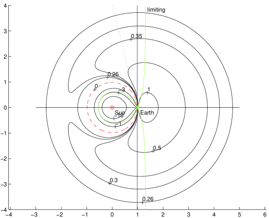
Figure 1: Level curves of $C(r,\rho)$ (solid lines), limiting curve (labeled), zero circle (dashed). For a given value of $C$ and an observation direction (dotted) there can be either 1 or 2 solutions, e.g. for $C=0.3$ there are 2.

Following [Charlier 1910, Charlier 1911] and [Plummer 1918] the number of solutions can be understood with the help of a plot of the level curves of $C(r,\rho)$, in a plane with the Sun at $(0,0)$, the Earth at $(q,0)$ and the position in each half-plane defined by the bipolar coordinates $(r,\rho)$. The limiting curve and the zero circle can be used to deduce the number of solutions occurring at the discovery of an object located at any point of the plane. There is only one solution on the right of the unlimited branches of the limiting curve, around opposition. There are two solutions for every point of the region between the unlimited branches and the zero circle. Inside the zero circle and outside the loop of the limiting curve there is only one solution. Inside that loop there are always two solutions.

Note that the classical theory by Charlier assumes that there is always at least one preliminary orbit solution. This results from two implicit assumptions: that the observed object exists (not being the result of a false identification) and that the value of $C$ is measured exactly, or at least to good accuracy, from the observations. $C$ contains $\kappa$ which can be difficult to measure from a short observed arc, thus both assumptions may fail as discussed in Section 5 and 6.2.

2.3 Gauss’ Method

The method by Gauss uses 3 observations corresponding to heliocentric positions

$$\mathbf{r}_{i}=\bm{\rho}_{i}+\mathbf{q}_{i}\ \ i=1,2,3$$ (10)

at times $t_{1}<t_{2}<t_{3}$ with $t_{i}-t_{j}={\cal O}(\Delta t)\ll$ period and the condition of coplanarity:

$$\lambda_{1}\mathbf{r}_{1}-\mathbf{r}_{2}+\lambda_{3}\mathbf{r}_{3}=0\ .$$ (11)

From (11)$\times\mathbf{r}_{i}\cdot\hat{\mathbf{c}}$, where $\mathbf{c}=\mathbf{r}_{i}\times\dot{\mathbf{r}}_{i}$, the coefficients $\lambda_{1},\,\lambda_{3}$ are obtained as triangle ratios

$$\lambda_{1}=\frac{\mathbf{r}_{2}\times\mathbf{r}_{3}\cdot\hat{\mathbf{c}}}{\mathbf{r}_{1}\times\mathbf{r}_{3}\cdot\hat{\mathbf{c}}}\ \ ;\ \ \lambda_{3}=\frac{\mathbf{r}_{1}\times\mathbf{r}_{2}\cdot\hat{\mathbf{c}}}{\mathbf{r}_{1}\times\mathbf{r}_{3}\cdot\hat{\mathbf{c}}}\ .$$

From (10) and $\hat{\bm{\rho}}_{1}\times\hat{\bm{\rho}}_{3}\cdot$(11):

$$\rho_{2}[\hat{\bm{\rho}}_{1}\times\hat{\bm{\rho}}_{3}\cdot\hat{\bm{\rho}}_{2}]=\hat{\bm{\rho}}_{1}\times\hat{\bm{\rho}}_{3}\cdot[\lambda_{1}\mathbf{q}_{1}-\mathbf{q}_{2}+\lambda_{3}\mathbf{q}_{3}].$$ (12)

Next, the differences $\mathbf{r}_{i}-\mathbf{r}_{2}$ are expanded in powers of $t_{ij}=t_{i}-t_{j}=O(\Delta t)$. e.g. by using the $f,g$ series formalism $\mathbf{r}_{i}=f_{i}\mathbf{r}_{2}+g_{i}\dot{\mathbf{r}}_{2}\;$ and Taylor expansions

$$f_{i}=1-\frac{\mu}{2}\frac{t_{i2}^{2}}{r_{2}^{3}}+{\cal O}(\Delta t^{3})\hskip 14.22636pt,\hskip 14.22636ptg_{i}=t_{i2}\left(1-\frac{\mu}{6}\frac{t_{i2}^{2}}{r_{2}^{3}}\right)+{\cal O}(\Delta t^{4})\ .$$ (13)

Then $\mathbf{r}_{i}\times\mathbf{r}_{2}=-g_{i}\mathbf{c}$, $\mathbf{r}_{1}\times\mathbf{r}_{3}=(f_{1}g_{3}-f_{3}g_{1})\mathbf{c}$ and

$$\lambda_{1}=\frac{g_{3}}{f_{1}g_{3}-f_{3}g_{1}}>0\ ;\ \lambda_{3}=\frac{-g_{1}}{f_{1}g_{3}-f_{3}g_{1}}>0$$ (14)

$$f_{1}g_{3}-f_{3}g_{1}=t_{31}\left(1-\frac{\mu}{6}\frac{t_{31}^{2}}{r_{2}^{3}}\right)+{\cal O}(\Delta t^{4})\ .$$ (15)

Using (13) and (15) in (14)

$$\lambda_{1}=\frac{t_{32}}{t_{31}}\left[1+\frac{\mu}{6r_{2}^{3}}(t_{31}^{2}-t_{32}^{2})\right]+{\cal O}(\Delta t^{3})\ .$$ (16)

$$\lambda_{3}=\frac{t_{21}}{t_{31}}\left[1+\frac{\mu}{6r_{2}^{3}}(t_{31}^{2}-t_{21}^{2})\right]+{\cal O}(\Delta t^{3})\ .$$ (17)

Let P be $3\times$volume of the pyramid with vertices $\mathbf{q},\mathbf{r}_{1},\mathbf{r}_{2},\mathbf{r}_{3}$ $P=\hat{\bm{\rho}}_{1}\times\hat{\bm{\rho}}_{2}\cdot\hat{\bm{\rho}}_{3}$; by substituting it and (16), (17) in (12), with simple manipulations of the times

$$-P\rho_{2}t_{31}=\hat{\bm{\rho}}_{1}\times\hat{\bm{\rho}}_{3}\cdot\left(t_{32}\mathbf{q}_{1}-t_{31}\mathbf{q}_{2}+t_{21}\mathbf{q}_{3}\right)+$$ (18)

$$+\hat{\bm{\rho}}_{1}\times\hat{\bm{\rho}}_{3}\cdot\left[\frac{\mu}{6r_{2}^{3}}[t_{32}t_{21}(t_{31}+t_{32})\mathbf{q}_{1}+t_{32}t_{21}(t_{31}+t_{21})\mathbf{q}_{3}]\right]+{\cal O}(\Delta t^{4})\ .$$

If the terms ${\cal O}(\Delta t^{4})$ are neglected and we let $B(\mathbf{q}_{1},\mathbf{q}_{3})$ represent the coefficient of the ${1}/{r_{2}^{3}}$ term in (18) then

$$B(\mathbf{q}_{1},\mathbf{q}_{3})=\frac{\mu}{6}t_{32}t_{21}\hat{\bm{\rho}}_{1}\times\hat{\bm{\rho}}_{3}\cdot[(t_{31}+t_{32})\mathbf{q}_{1}+(t_{31}+t_{21})\mathbf{q}_{3}].$$ (19)

Then multiply (18) by ${q_{2}^{3}}/{B(\mathbf{q}_{1},\mathbf{q}_{3})}$ to obtain

$$-\frac{P\;\rho_{2}\;t_{31}}{B(\mathbf{q}_{1},\mathbf{q}_{3})}\;q_{2}^{3}=\frac{q_{2}^{3}}{r_{2}^{3}}+\frac{A(\mathbf{q}_{1},\mathbf{q}_{2},\mathbf{q}_{3})}{B(\mathbf{q}_{1},\mathbf{q}_{3})}$$

where

$$A(\mathbf{q}_{1},\mathbf{q}_{2},\mathbf{q}_{3})=q_{2}^{3}\;\hat{\bm{\rho}}_{1}\times\hat{\bm{\rho}}_{3}\cdot[t_{32}\mathbf{q}_{1}-t_{31}\mathbf{q}_{2}+t_{21}\mathbf{q}_{3}].$$ (20)

Let

$$C_{0}=\frac{P\;t_{31}\;q_{2}^{4}}{B(\mathbf{q}_{1},\mathbf{q}_{3})}\hskip 14.22636pt,\hskip 14.22636pth_{0}=-\frac{A(\mathbf{q}_{1},\mathbf{q}_{2},\mathbf{q}_{3})}{B(\mathbf{q}_{1},\mathbf{q}_{3})}$$

and then

$$C_{0}\,\frac{\rho_{2}}{q_{2}}=h_{0}-\frac{q_{2}^{3}}{r_{2}^{3}}$$ (21)

is the dynamical equation of Gauss’ method, similar (but not identical) to eq. (5) of Laplace’s method. Using (7) at time $t_{2}$ (with $q_{2}$, $\rho_{2}$, $r_{2}$ and $\varepsilon_{2}$):

$$P_{0}(r)=C_{0}^{2}r_{2}^{8}-q_{2}^{2}r_{2}^{6}(h_{0}^{2}+2C_{0}h_{0}\cos{\varepsilon_{2}}+C_{0}^{2})+2q_{2}^{5}r_{2}^{3}(h_{0}+C_{0}\cos{\varepsilon_{2}})-q_{2}^{8}=0$$ (22)

where the sign of the coefficients is as for (8), apart from $h_{0}+C_{0}\cos{\varepsilon_{2}}$ whose sign may change depending upon $h_{0}$. Note that $P_{0}(q)\neq 0$, no root can be found analytically. The number of positive roots is still $\leq 3$ but a qualitative theory such as the one of Section 2.2 is not available in the literature.

After the possible values for $r_{2}$ have been found the corresponding $\rho_{2}$ values are obtained from eq. (21) and the velocity $\dot{\mathbf{r}}_{2}$ can be computed, e.g. from the classical formulae by Gibbs [Herrick 1971, Chap. 8].

3 Topocentric Gauss-Laplace Methods

The critical difference between the methods of Gauss and Laplace is the following. Gauss uses a truncation (to order ${\cal O}(\Delta t^{2})$) in the motion $\mathbf{r}(t)$ of the asteroid but the positions of the observer (be it coincident with the center of the Earth or not) are used in their exact values. Laplace uses a truncation to the same order of the relative motion $\bm{\rho}(t)$, thus implicitly approximating the motion of the observer. In this section we examine the consequences of the difference between the techniques.

3.1 Gauss-Laplace equivalence

To directly compare the two methods let us introduce in Gauss’ method the same approximation to order ${\cal O}(\Delta t^{2})$ in the motion of the Earth which is still assumed to coincide with the observer. The $f$, $g$ series for Earth are

$$\mathbf{q}_{i}=\left(1-\frac{\mu}{2}\frac{t_{i2}^{2}}{q_{2}^{3}}\right)\mathbf{q}_{2}+t_{i2}\dot{\mathbf{q}}_{2}+\frac{\mu}{6}\frac{t_{i2}^{3}}{q_{2}^{3}}\left[\frac{3(\mathbf{q}_{2}\cdot\dot{\mathbf{q}}_{2})\mathbf{q}_{2}}{q_{2}^{2}}-\dot{\mathbf{q}}_{2}\right]+{\cal O}(\Delta t^{4})$$ (23)

By using (23) in (19) we find that

$$B(\mathbf{q}_{1},\mathbf{q}_{3})=\frac{\mu}{6}t_{32}t_{21}\hat{\bm{\rho}}_{1}\times\hat{\bm{\rho}}_{3}\cdot[3t_{31}\mathbf{q}_{2}+t_{31}(t_{32}-t_{21})\dot{\mathbf{q}}_{2}+{\cal O}(\Delta t^{3})].$$

If $\ t_{32}-t_{21}=t_{3}+t_{1}-2t_{2}=0$, implying that the interpolation for ${d^{2}}/{dt^{2}}$ is done at the central value $t_{2}$, then

$$B(\mathbf{q}_{1},\mathbf{q}_{3})=\frac{\mu}{2}t_{21}t_{32}t_{31}\hat{\bm{\rho}}_{1}\times\hat{\bm{\rho}}_{3}\cdot\mathbf{q}_{2}\;(1+{\cal O}(\Delta t^{2}))\ ;$$

else, if $t_{2}\neq(t_{1}+t_{3})/2$ the last factor is just $(1+{\cal O}(\Delta t))$. Using (23) in (20)

$$A(\mathbf{q}_{1},\mathbf{q}_{2},\mathbf{q}_{3})=\hat{\bm{\rho}}_{1}\times\hat{\bm{\rho}}_{3}\cdot\left\{-\frac{\mu}{2}t_{21}t_{32}t_{31}\mathbf{q}_{2}+\right\}$$

$$\left.+\frac{\mu}{6}t_{21}t_{32}t_{31}(t_{32}-t_{21})\left[\frac{3(\mathbf{q}_{2}\cdot\dot{\mathbf{q}}_{2})\mathbf{q}_{2}}{q_{2}^{2}}-\dot{\mathbf{q}}_{2}\right]+{\cal O}(\Delta t^{5})\right\}.$$

If, as above, $t_{32}+t_{12}=t_{3}+t_{1}-2t_{2}=0$ then

$$A(\mathbf{q}_{1},\mathbf{q}_{2},\mathbf{q}_{3})=-\frac{\mu}{2}t_{21}t_{32}t_{31}\hat{\bm{\rho}}_{1}\times\hat{\bm{\rho}}_{3}\cdot\mathbf{q}_{2}\;(1+{\cal O}(\Delta t^{2}))$$

and we can conclude

$$h_{0}=-\frac{A}{B}=1+{\cal O}(\Delta t^{2})\ .$$

To compute $P$ we need

$$\frac{d^{2}\hat{\bm{\rho}}}{dt^{2}}=\frac{d\dot{\hat{\bm{\rho}}}}{dt}=\frac{d}{dt}(\eta\hat{\mathbf{v}})=-\eta^{2}\hat{\bm{\rho}}+\dot{\eta}\hat{\mathbf{v}}+\kappa\eta^{2}\hat{\mathbf{n}}$$ (24)

to make a Taylor expansion of $\hat{\bm{\rho}}_{i}$ in $t_{2}$

$$\hat{\bm{\rho}}_{i}=\hat{\bm{\rho}}_{2}+t_{i2}\eta\hat{\mathbf{v}}_{2}+\frac{t_{i2}^{2}}{2}(-\eta^{2}\hat{\bm{\rho}}_{2}+\dot{\eta}\hat{\mathbf{v}}_{2}+\kappa\eta^{2}\hat{\mathbf{n}}_{2})+{\cal O}(\Delta t^{3}).$$

This implies that

$$\hat{\bm{\rho}}_{1}\times\hat{\bm{\rho}}_{3}\cdot\hat{\bm{\rho}}_{2}=\frac{1}{2}\,\left[t_{12}\eta\hat{\mathbf{v}}_{2}\times t_{32}^{2}\kappa\,\eta^{2}\hat{\mathbf{n}}_{2}-t_{32}\eta\,\hat{\mathbf{v}}_{2}\times t_{12}^{2}\kappa\,\eta^{2}\,\hat{\mathbf{n}}_{2}\right]\cdot\hat{\bm{\rho}}_{2}+{\cal O}(\Delta t^{5})$$

and the ${\cal O}(\Delta t^{4})$ term vanishes thus

$$P=-\frac{\kappa\eta^{3}}{2}(t_{12}t_{32}^{2}-t_{32}t_{12}^{2})\;(1+{\cal O}(\Delta t^{2}))=\frac{\kappa\eta^{3}}{2}t_{21}t_{32}t_{31}\;(1+{\cal O}(\Delta t^{2}))$$

and

$$C_{0}=\frac{Pt_{31}q_{2}^{4}}{B}=\frac{\kappa\eta^{3}t_{31}q_{2}^{4}+{\cal O}(\Delta t^{3})}{\mu\hat{\bm{\rho}}_{1}\times\hat{\bm{\rho}}_{3}\cdot\mathbf{q}_{2}\,(1+{\cal O}(\Delta t))}.$$ (25)

In the denominator $\hat{\bm{\rho}}_{1}\times\hat{\bm{\rho}}_{3}$ computed to order $\Delta t^{2}$ is

$$\hat{\bm{\rho}}_{1}\times\hat{\bm{\rho}}_{3}=t_{31}\,\eta\,\hat{\mathbf{n}}_{2}+\frac{t_{32}^{2}-t_{12}^{2}}{2}\;(\dot{\eta}\,\hat{\mathbf{n}}_{2}-\kappa\,\eta^{2}\,\hat{\mathbf{v}}_{2})+{\cal O}(\Delta t^{3}).$$ (26)

If $t_{32}-t_{21}=t_{3}+t_{1}-2t_{2}=0$ then

$$C_{0}=\frac{\kappa\,\eta^{3}\,t_{31}q_{2}^{4}+{\cal O}(\Delta t^{3})}{\mu\,t_{31}\,\eta\,q_{2}\hat{\mathbf{q}}_{2}\cdot\hat{\mathbf{n}}_{2}+{\cal O}(\Delta t^{3})}=\frac{\kappa\,\eta^{2}\,q_{2}^{3}}{\mu\,\hat{\mathbf{q}}_{2}\cdot\hat{\mathbf{n}}_{2}}\;(1+({\cal O}\Delta t^{2}))\ ,$$

otherwise the last factor is $(1+{\cal O}(\Delta t))$.

We can conclude that if the topocentric correction is neglected the coefficients of the two dynamical equations (5) and (21) are the same to zero order in $\Delta t$ and also to order 1 if the time $t_{2}$ is the average time.

3.2 Topocentric Correction in Laplace’s Method

Now let us remove the approximation that the observer sits at the center of the Earth and introduce the topocentric correction into Laplace’s method. The center of mass of the Earth is at $\mathbf{q}_{\oplus}$ but the observer is at $\mathbf{q}=\mathbf{q}_{\oplus}+\mathbf{P}$. Let us derive the dynamical equation by also taking into account the acceleration contained in the geocentric position of the observer $\mathbf{P}(t)$ such that

$$\frac{d^{2}\bm{\rho}}{dt^{2}}=-\frac{\mu\mathbf{r}}{r^{3}}+\frac{\mu\mathbf{q}_{\oplus}}{q_{\oplus}^{3}}-\ddot{\mathbf{P}}.$$

Multiplying by $\cdot\hat{\mathbf{n}}$ and using eq. (3)

$$\frac{d^{2}\bm{\rho}}{dt^{2}}\cdot\hat{\mathbf{n}}=\rho\eta^{2}\kappa=\mu\left[q_{\oplus}\frac{\hat{\mathbf{q}}_{\oplus}\cdot\hat{\mathbf{n}}}{q_{\oplus}^{3}}-q_{\oplus}\frac{\hat{\mathbf{q}}_{\oplus}\cdot\hat{\mathbf{n}}}{r^{3}}-P\,\frac{\hat{\mathbf{P}}\cdot\hat{\mathbf{n}}}{r^{3}}\right]-\ddot{\mathbf{P}}\cdot\hat{\mathbf{n}}$$

The term $P\,{\hat{\mathbf{P}}\cdot\hat{\mathbf{n}}}/{r^{3}}$ can be neglected. This approximation is legitimate because $P/q_{\oplus}\leq 4.3\times 10^{-5}$ and the neglected term is smaller than the planetary perturbations. Thus

$$C\frac{\rho}{q_{\oplus}}=(1-\Lambda_{n})-\frac{q_{\oplus}^{3}}{r^{3}}$$ (27)

where

$$C=\frac{\eta^{2}\kappa q_{\oplus}^{3}}{\mu\hat{\mathbf{q}}_{\oplus}\cdot\hat{\mathbf{n}}}\hskip 14.22636pt,\hskip 14.22636pt\Lambda_{n}=\frac{q_{\oplus}^{2}\ddot{\mathbf{P}}\cdot\hat{\mathbf{n}}}{\mu\hat{\mathbf{q}}_{\oplus}\cdot\hat{\mathbf{n}}}=\frac{\ddot{\mathbf{P}}\cdot\hat{\mathbf{n}}}{({\mu}/{q_{\oplus}^{2}})\,\hat{\mathbf{q}}_{\oplus}\cdot\hat{\mathbf{n}}}.$$ (28)

Note that $\Lambda_{n}$ is singular only where $C$ is also singular. The analog of eq. (6), again neglecting ${\cal O}(p/q_{\oplus})$, is

$$\rho\dot{\eta}+2\dot{\rho}\eta=\frac{\mu\;\hat{\mathbf{q}}_{\oplus}\cdot\hat{\mathbf{v}}}{q_{\oplus}^{2}}\;\left(1-\Lambda_{v}-\frac{q_{\oplus}^{3}}{r^{3}}\right)\hskip 14.22636pt,\hskip 14.22636pt\Lambda_{v}=\frac{q_{\oplus}^{2}\;\ddot{\mathbf{P}}\cdot\hat{\mathbf{v}}}{\mu\;\hat{\mathbf{q}}_{\oplus}\cdot\hat{\mathbf{v}}}\ .$$ (29)

The important fact is that $\Lambda_{n}$ and $\Lambda_{v}$ are by no means small. The centripetal acceleration of the observer (towards the rotation axis of the Earth) has size $\Omega_{\oplus}^{2}\,R_{\oplus}\,\cos\theta$ where $\Omega_{\oplus}$ is the angular velocity of the Earth’s rotation, $R_{\oplus}$ the radius of the Earth and $\theta$ the latitude; the maximum of $\simeq 3.4\;cm\,s^{-2}$ occurs at the equator. The quantity ${\mu}/{q_{\oplus}^{2}}$ in the denominator of $\Lambda_{n}$ is the size of the heliocentric acceleration of the Earth, $\simeq 0.6\;cm\,s^{-2}$. Thus $|\Lambda_{n}|$ can be $>1$, and the coefficient $1-\Lambda_{n}$ very different from $1$; it may even be negative. This leads to the conclusion that without taking into account the topocentric correction the classical method of Laplace is not a good approximation in the general case.

The common procedure when using Laplace’s method is to apply a negative topocentric correction to go back to the geocentric observation case. However, in doing this some value of $\rho$ is assumed as a first approximation. If this value is approximately correct, by iterating the cycle (topocentric correction - Laplace’s determination of $\rho$) convergence is achieved. If the starting value is really wrong the procedure may well diverge. (e.g. a value $\rho=1\,AU$ is assumed by default and the object is actually undergoing a close approach to the Earth). Moreover, in this way the information contained in the parallax is not exploited in an optimal way. Unless a better way is found to account for the topocentric correction there are reliability problems discouraging the use of Laplace’s method when processing a large dataset, containing discoveries of objects of different orbital classes and therefore spanning a wide range of distances.

3.3 Gauss-Laplace equivalence, Topocentric

When taking into account the displacement $\mathbf{P}$ the Taylor expansion of $\mathbf{q}_{i}(t)$ of eq. (23) is not applicable. We need to use

$$\mathbf{q}_{i}=\mathbf{q}_{2}+t_{i2}\dot{\mathbf{q}}_{2}+\frac{t_{i2}^{2}}{2}\ddot{\mathbf{q}}_{2}+{\cal O}(\Delta t^{3})$$

where $\mathbf{q}_{2}(t)$ and its derivatives contain also $\mathbf{P}(t)$. By using eq. (26) and assuming $t_{21}=t_{32}$, eq. (19) and (20) become

$$B(\mathbf{q}_{1},\mathbf{q}_{3})=\frac{\mu\;\eta}{2}\;t_{21}t_{32}t_{31}^{2}\;\hat{\mathbf{n}}_{2}\cdot\mathbf{q}_{2}+{\cal O}(\Delta t^{6})$$

$$A(\mathbf{q}_{1},\mathbf{q}_{2},\mathbf{q}_{3})=\frac{q_{2}^{3}\;\eta}{2}\;t_{21}t_{32}t_{31}^{2}\;\hat{\mathbf{n}}_{2}\cdot\ddot{\mathbf{q}}_{2}+{\cal O}(\Delta t^{6})\ .$$

Note that $\dot{\mathbf{q}}_{2}$ does not appear in $A$ at this approximation level. Thus

$$h_{0}=-\frac{A}{B}=-\frac{q_{2}^{3}\ \hat{\mathbf{n}}_{2}\cdot\ddot{\mathbf{q}}_{2}+{\cal O}(\Delta t^{2})}{\mu\ \hat{\mathbf{n}}_{2}\cdot\mathbf{q}_{2}+{\cal O}(\Delta t^{2})}$$

and once again neglecting $P/q_{\oplus}$ terms

$$=-\frac{q_{2}^{3}\ \hat{\mathbf{n}}_{2}\cdot\ddot{\mathbf{q}}_{\oplus 2}}{\mu\ \hat{\mathbf{n}}_{2}\cdot\mathbf{q}_{2}}-\frac{q_{2}^{3}\ \hat{\mathbf{n}}_{2}\cdot\ddot{\mathbf{P}}_{2}}{\mu\ \hat{\mathbf{n}}_{2}\cdot\mathbf{q}_{2}}+O(\Delta t^{2})=$$

$$=\frac{q_{2}^{3}}{q_{\oplus 2}^{3}}-\frac{q_{2}^{3}\ \hat{\mathbf{n}}_{2}\cdot\ddot{\mathbf{P}}_{2}}{\mu\ \hat{\mathbf{n}}_{2}\cdot\mathbf{q}_{2}}+{\cal O}(\Delta t^{2}).$$

Finally

$$\hat{\mathbf{n}}_{2}\cdot\mathbf{q}_{2}=q_{2}\ \hat{\mathbf{n}}_{2}\cdot\left(\frac{\mathbf{q}_{\oplus 2}}{q_{2}}+\frac{\mathbf{P}_{2}}{q_{2}}\right)=q_{2}\left(\hat{\mathbf{n}}_{2}\cdot\hat{\mathbf{q}}_{\oplus 2}+{\cal O}\left(\frac{P_{2}}{q_{2}}\right)\right)$$

then

$$h_{0}=1-\frac{q_{\oplus 2}^{3}\ \hat{\mathbf{n}}_{2}\cdot\ddot{\mathbf{P}}_{2}}{\mu\ \hat{\mathbf{n}}_{2}\cdot\mathbf{q}_{2}}+{\cal O}(\Delta t^{2})+{\cal O}\left(\frac{P_{2}}{q_{2}}\right)=1-\Lambda_{n2}+{\cal O}(\Delta t^{2})+{\cal O}\left(\frac{P_{2}}{q_{2}}\right)$$

where $\Lambda_{n2}$ is the same quantity as $\Lambda_{n}$ given by eq. (28) and computed at $t=t_{2}$.

The conclusion is that Gauss’ method used with the heliocentric positions of the observer $\mathbf{q}_{i}$ is equivalent to Laplace’s method with topocentric correction to lowest order in $\Delta t$ and neglecting the very small term ${\cal O}({P_{2}}/{q_{2}})$.

3.4 Problems in Topocentric Laplace’s Method

The results obtained in this Section can be summarized as follows: contrary to common belief, Gauss’ method is not equivalent to Laplace’s unless Gauss’ is artificially spoiled by not using the observer position in eq. (19) and (20). In its rigorous form, Gauss’ method accounts for the topocentric correction with a consistent approximation. The question arises whether we could account for the topocentric correction in Laplace’s method (without iterations) by adding the term $\Lambda_{n}$ from eq. (28). Surprisingly, the answer is already contained in the literature in a 100 year old paper by a famous author [Poincaré 1906, pag. 177–178]. To summarize the argument of Poincaré, plots showing the shape of the topocentric corrections as a function of time and a short citation are enough.

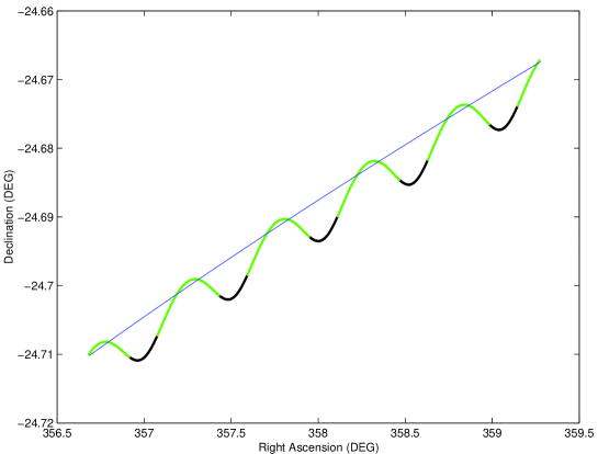
Figure 2: The path in the sky of an approaching NEO. This example is (101955) 1999 RQ₃₆ as it would have been seen in July 2005 if an observatory on Mauna Kea had been observing continously. The curve resembling a parabola gives simulated observations from the geocenter.

Figure 2 shows the simulated path of an approaching NEO as seen from an observing station (in this example in Hawaii). The darker portions of the curve indicate possible observations that have an altitude $>15^{\circ}$. The overall apparent motion of the asteroid from night to night cannot be approximated using parabolic motion segments fitted to a single night. For the geocentric path the parabolic approximation to $\hat{\bm{\rho}}(t)$, used by Laplace, would be applicable.

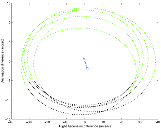
Figure 3: The same data as in the previous figure after removing the best fitting linear functions of time in both coordinates. In this case the curves represent the content of information beyond the attributable. The larger loop is from Mauna Kea while the small curl near $(0,0)$ is for a geocentric observer. Coordinates are differences in RA and DEC in radians.

Figure 3 shows graphically that topocentric observations contain information beyond what is contained in the average angles and proper motion (the attributable, see Section 5). Thus, to reduce the observations to the geocenter by removing the topocentric correction is not a good strategy.

Poincaré suggests computing what we call $\Lambda_{n}$ by using a value of $\ddot{\mathbf{P}}$ obtained by interpolating the values $\mathbf{P}(t_{i})$ at the times $t_{i}$ of the observations which are not limited to 3 (one of the advantages of Laplace’s method). We have implemented Poincaré’s suggestion to improve Laplace’s method in our software system OrbFit but we still need to test it properly.

When the observations are performed from an artificial satellite (such as the Space Telescope or, in the future, from Gaia) the acceleration $\ddot{\mathbf{P}}\simeq 900\;cm\;s^{-2}$ and the $\Lambda_{n}$ and $\Lambda_{v}$ coefficients can be up to $\simeq 1,500$. A few hours of observations extending to several orbits can produce multiple kinks as in [Marchi et al. 2004, Figure 1] containing important orbital information.

4 Qualitative Theory, Topocentric

In rectangular heliocentric coordinates $(x,y)$ where the $x$ axis is along $\hat{\mathbf{q}}_{2}$ (from the Sun to the observer) we have $\rho_{2}=\sqrt{q_{2}^{2}+x^{2}+y^{2}-2xq_{2}}$ and $r_{2}=\sqrt{x^{2}+y^{2}}$, thus we can consider the function

$$C_{0}(x,y)=\frac{q_{2}}{\sqrt{q_{2}^{2}+x^{2}+y^{2}-2xq_{2}}}\left[h_{0}-\frac{q_{2}^{3}}{(x^{2}+y^{2})^{3/2}}\right]\ .$$

The dynamical equation eq. (21) can be seen as describing the level lines $C_{0}=const$ in a bipolar coordinate system $(r_{2},\rho_{2})$. Note that $C_{0}=0$ is the zero circle $r=r_{0}=q/\sqrt[3]{h_{0}}$ for $h_{0}>0$ and is otherwise empty. A simple computation of the partial derivatives of $C_{0}$ shows that the only stationary points of $C_{0}$ are the pairs $(x,y)$ with $y=0$ and $x$ a solution of the equation $(h_{0}|x|^{3}-q_{2}^{3})x=3q_{2}^{3}(x-q_{2})$. For $h_{0}\leq 0$ it has only one solution, $x_{1}$, with $0<x_{1}<q_{2}$. For $h_{0}>0$ there is always at least one solution $\bar{x}<-r_{0}<0$. If $0<h_{0}<1$ there are two additional solutions, $x_{1}$ and $x_{2}$ such that $0<x_{1}<q_{2}<r_{0}<x_{2}$. For $h_{0}>1$ there are no positive solutions.

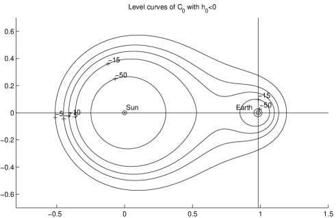
Figure 4: Level curves of $C_{0}(x,y)$ for $h_{0}=-0.5$. Note there is no zero circle.

The function $C_{0}(x,y)$ has a pole of order 3 at $(x,y)=(0,0)$, with $\lim_{r_{2}\to 0}C_{0}=-\infty$, and a pole of order 1 at $(q_{2},0)$ with $\lim_{r_{2}\to 0}C_{0}=+\infty$ for $h_{0}>1$ and $=-\infty$ for $h_{0}<1$. For $h_{0}=1$ there is at $(q_{2},0)$ a more complicated singularity: as shown by Figure 1 there is no unique limit value for $\rho_{2}\to 0$.

4.1 Topology of the level curves of $C_{0}(x,y)$

The qualitative behavior of the level lines of $C_{0}(x,y)$ is different in the three cases $h_{0}\leq 0$ (Figure 4), $0<h_{0}<1$ (Figure 5) and $h_{0}>1$ (Figure 6).

The number of solutions of the dynamical equation (i.e. along a fixed topocentric direction) can be understood by evaluating the degree 8 polynomial (22) on the zero circle

$$P(r_{0})=C_{0}^{2}\;\frac{q^{8}}{h_{0}^{8/3}}\;\left(1-h_{0}^{2/3}\right)\ .$$

Table 1: The number of preliminary orbit solutions, the columns give: [1] the number of preliminary orbit solutions (for a given $C$ and $\epsilon$), [2] the number of positive roots of the polynomial equation (22), [3] the number of spurious roots.

		[1]	[2]	[3]
$h_{0}\leq 0$	${\cal C}<0$	1 or 3	1 or 3	0
	${\cal C}>0$	0	1 or 3	1 or 3
$0<h_{0}<1$	${\cal C}<0$	1 or 3	1 or 3	0 or 2
	${\cal C}>0$	0 or 2	1 or 3	1 or 3
$h_{0}=1$	${\cal C}<0$	0 or 1 or 2	1 or 3	1 or 2 or 3
	${\cal C}>0$	0 or 1 or 2	1 or 3	1 or 2 or 3
$h_{0}>1$	${\cal C}<0$	0 or 2	1 or 3	1 or 3
	${\cal C}>0$	1 or 3	1 or 3	0 or 2

We summarize the possible numbers of solutions, for a given direction of observation $\epsilon$, in the different cases, depending upon the value of $h_{0}$ and the sign of $C$, in Table 1. Note that in the Table we are not making the assumption of Charlier, that some solutions must exist, for the reasons given in Section 2.2. By spurious we mean a root of the polynomial (22) corresponding to $\rho\leq 0$ in eq. (21). This is not a complete qualitative theory replacing Charlier’s for $h_{0}=1$, but already shows that the number of solutions can be quite different from the classical case e.g. , 2 solutions near opposition and up to 3 at low elongation. For a fully generalized qualitative theory see [Gronchi 2007].

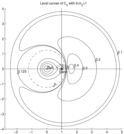
Figure 5: Level curves of $C_{0}(x,y)$ for $h_{0}=0.5$, including the zero circle (dashed).

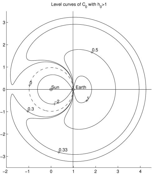
Figure 6: Level curves of $C_{0}(x,y)$ for $h_{0}=1.1$, including the zero circle (dashed).

4.2 Examples

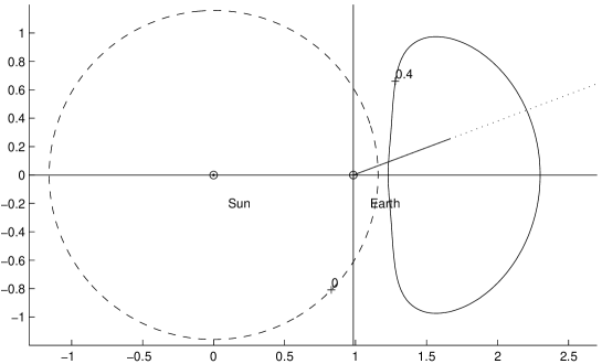
Figure 7: An example with two solutions near opposition: for $h_{0}=0.613$ the direction of observation (dotted) has two intersections with the level curve $C_{0}(x,y)=0.4$ (continuous); the zero circle is dashed. The positions in the observation direction with a bounded orbit are drawn as a continuous line.

We would like to find examples in which the additional solutions with respect to the classical theory by Charlier are useful. That is, cases in which the additional solutions provide a preliminary orbit closer to the true orbit and therefore more suitable as a first guess for the differential corrections procedure.

An example in which there are two solutions while observing in a direction close to the opposition is shown in Figure 7. Of the two intersections of the observing half line with the relevant level curve of $C_{0}$, the one leading to a useful preliminary orbit is the nearer one which has $\rho_{2}=0$ as counterpart in the classical theory. The farther one leads to a preliminary orbit with $e\simeq 10$. We have used the formulae of [Milani et al. 2004] to compute the maximum possible $\rho_{2}$ along the observation direction compatible with $e\leq 1$.

Another interesting feature of this example is that the preliminary orbit using the nearer solution has residuals of the 6 observations with RMS $=66$ arcsec while the one using the farther solution has RMS $=2.5$ arcsec. This implies that if only one preliminary solution were passed to the next processing step by selecting the one with lowest RMS the good solution would be discarded.

Figure 8: For the preliminary orbit of 2002 AA₂₉ the relevant level curve ($C_{0}=1.653$) is shown (continuous) in the same plane of Figure 1; the zero circle (dashed) and the observation direction (dotted) are also shown. Left: using the actual value $h_{0}=1.025$. Right: using a value of $h_{0}=1$ that does not account for the topocentric correction.

To find a significant example with 3 solutions is not easy because in many cases the third solution, the nearest to the observer, has $\rho_{2}$ too small for the heliocentric 2-body approximation to be applicable. A value $\rho_{2}\leq 0.01$ AU corresponds to the sphere of influence of the Earth, i.e., the region where the “perturbation” from the Earth is actually more important that the attraction from the Sun. Thus, a solution with such a small $\rho_{2}$ must be discarded, because the approximation used in Gauss’ and Laplace’s method is not valid.

To show how our arguments on the number of solutions applies to a real case (as opposed to a simulation as in the example above) we have selected the asteroid 2002 AA₂₉ and used observations from the first three nights (9, 11 and 12 January 2002). With the values $C_{0}=1.653\;,\;h_{0}=1.025$ we obtain from the observations and an elongation $\simeq 111^{\circ}$ there is only one solution with $\rho_{2}=0.0045$ (see Figure 8, left), which easily leads to a full least squares solution with $\rho_{2}=0.044$. Although the value of $h_{0}$ is not very far from 1 the existence of the solution depends critically on $h_{0}-1\neq 0$. If the value of $h_{0}$ had been set to 1 we would find no solution (see Figure 8, right).

4.3 Implementation issues

We need to implement the algorithms discussed in this paper for the computation of preliminary orbits in a way which is suitable for a large observation data set; we need to satisfy three requirements.

The first requirement is to obtain the solutions to the polynomial equations such as (22) in a way which is fast and reliable in providing the number of distinct real solutions. In this way we can fully exploit the understanding on the number of solutions (with topocentric correction) which we have achieved in this section. This is made possible by the algorithms computing the set of roots of a polynomial equation at once (as a complex vector) and with rigorous upper bounds for the errors including the ones generated by roundoff. We use the algorithm by [Bini 1996] and the corresponding public domain software.

The second requirement is to improve the preliminary orbit as obtained from the solutions of the degree 8 polynomial equations in such a way that it is as close as possible to the “true” solution to be later obtained by differential corrections. There is such an immense literature on this topic that in this paper it is not even appropriate to discuss the references. Conceptually, as shown by [Celletti and Pinzari 2005], each step in the iterative procedures used in differential corrections can be shown to increase the order in $\Delta t$ of the approximation to the exact solutions of the 2-body equations of motion. However, [Celletti and Pinzari 2006] have also shown that an iterative Gauss map can diverge when the solution of the degree 8 equation is far from the fixed point of the iterative procedure, outside of its convergence domain.

We have implemented one of the available iterative improvement algorithms for Gauss’ method and have found that it provides in most cases a preliminary orbit much closer to the least squares solution and therefore a more reliable first guess for the least squares algorithms. We have also found that the Gauss map diverges in a small fraction of the test cases but still often enough to significantly decrease the efficiency of the algorithm. In some cases the number of orbits for which the Gauss map converges is less than the number of solutions of the degree 8 equations. It can happen that one of the lost degree 8 solutions was the one closest to the “true” orbit and the only one which can be used to obtain the best least squares solutions. One method to obtain the highest efficiency without an inordinate increase in the computational cost is to run two iterations, one with and one without the Gauss map.

The third requirement is to use modified differential corrections iterative algorithms with larger convergence domains in such a way that even when the geodetic curvature (contained in the coefficients $C$ and $C_{0}$ of the two methods) is poorly constrained by the available observations (because the arc length on the celestial sphere is too short) the very rough preliminary orbit solution can lead to a least squares solution. This is discussed in the next section.

5 Weak preliminary orbits

An essential difference between the classical works on preliminary orbits and the modern approach to the same problem is that the effects of the astrometric errors cannot be neglected, especially in the operating condition of modern surveys: they use shorter observed arcs, thus the deviations of the observed path on the celestial sphere from a great circle may not be significant.

5.1 Uncertainty of Curvature

The explicit computation of the two components of curvature of interest for orbit determination, geodesic curvature $\kappa$ and along track acceleration $\dot{\eta}$, can be performed by using the properties of the orthonormal frame (1) by straightforward computation using the Riemannian structure of the unit sphere [Milani et al. 2006b, Section 6.4]. The results are

$$\kappa = \frac{1}{\eta^{3}}\;\left\{(\ddot{\delta}\;\dot{\alpha}-\ddot{\alpha}\;\dot{\delta})\;\cos\delta+\dot{\alpha}\;\left[\eta^{2}+(\dot{\delta})^{2}\right]\;\sin\delta\right\}=\kappa(\alpha,\delta,\dot{\alpha},\dot{\delta},\ddot{\alpha},\ddot{\delta})\ \ \$$ (30)

$$\dot{\eta} = \frac{1}{\eta}\;\left[\ddot{\alpha}\;\dot{\alpha}\;\cos^{2}\delta+\ddot{\delta}\;\dot{\delta}-(\dot{\alpha})^{2}\;\dot{\delta}\;\cos\delta\;\sin\delta\right]=\dot{\eta}(\alpha,\delta,\dot{\alpha},\dot{\delta},\ddot{\alpha},\ddot{\delta})\ .$$ (31)

Given these explicit formulae it is possible to compute the covariance matrix of the quantities $(\kappa,\dot{\eta})$ by propagation of the covariance matrix of the angles and their derivatives with the matrix of partial derivatives for $\kappa$ and $\dot{\eta}$

$$\Gamma_{\kappa,\dot{\eta}}=\frac{\partial(\kappa,\dot{\eta})}{\partial(\alpha,\delta,\dot{\alpha},\dot{\delta},\ddot{\alpha},\ddot{\delta})}\;\Gamma_{\alpha,\delta}\;\left[\frac{\partial(\kappa,\dot{\eta})}{\partial(\alpha,\delta,\dot{\alpha},\dot{\delta},\ddot{\alpha},\ddot{\delta})}\right]^{T}\ .$$ (32)

The covariance matrix $\Gamma_{\alpha,\delta}$ for the angles and their first and second derivatives is obtained by the procedure of least squares fit of the individual observations to a quadratic function of time. The partials of $\kappa$ and $\dot{\eta}$ are given below (note that the partials with respect to $\alpha$ are zero).

$$\frac{\partial\kappa}{\partial\delta} = -\frac{1}{\eta^{5}}\Bigl{[}-2\,{{\it\dot{\alpha}}}^{3}\cos^{2}\delta\;\sin\delta\;{\it\ddot{\delta}}+\sin\delta\;\ddot{\delta}\,\dot{\alpha}\,{\dot{\delta}}^{2}+2\,{\dot{\alpha}}^{2}\cos^{2}\delta\;\sin\delta\;{\ddot{\alpha}}\,\dot{\delta}-$$

$$- \sin\delta\;{\it\ddot{\alpha}}\,{{\it\dot{\delta}}}^{3}-{{\it\dot{\alpha}}}^{5}\cos^{3}\delta\;-4\,{{\it\dot{\alpha}}}^{3}\cos\delta\;{{\it\dot{\delta}}}^{2}+{{\it\dot{\alpha}}}^{3}\cos^{3}\delta\;{\dot{\delta}}^{2}-2\,{\it\dot{\alpha}}\,\cos\delta\;{\dot{\delta}}^{4}\Bigr{]}$$

$$\frac{\partial\dot{\eta}}{\partial\delta}=-\frac{\dot{\alpha}}{2\;\eta^{3}}\Bigl{[}\sin(2\delta)\,\left({\dot{\alpha}}^{2}\;\ddot{\alpha}\;\cos^{2}\delta+2\;{\dot{\delta}}^{2}\;\ddot{\alpha}-\dot{\alpha}\;\dot{\delta}\;\ddot{\delta}\right)+2\,\dot{\alpha}\;{\dot{\delta}}^{3}\,\cos(2\delta)+2\,{\dot{\alpha}}^{3}\dot{\delta}\;\cos^{4}\delta\Bigr{]}$$

$$\frac{\partial\kappa}{\partial\dot{\alpha}}=\frac{1}{\eta^{5}}\left[-\dot{\alpha}\;\cos^{3}\delta\,\left(2\,\dot{\alpha}\;\ddot{\delta}-3\,\dot{\delta}\;\ddot{\alpha}\right)+{\dot{\delta}}^{2}\,\left(\ddot{\delta}\,\cos\delta-{\dot{\alpha}}^{2}\cos^{2}\delta\;\sin\delta+2\,{\dot{\delta}}^{2}\;\sin\delta\right)\right]$$

$$\frac{\partial\dot{\eta}}{\partial\dot{\alpha}}=-\frac{\cos\delta\;\;\dot{\delta}}{\eta^{3}}\;\left[\,-\cos\delta\;{\;\ddot{\alpha}}\,\dot{\delta}+{\dot{\alpha}}^{3}\sin\delta\;\cos^{2}\delta\;+2\,{\dot{\alpha}}\,\sin\delta\;{\dot{\delta}}^{2}+\cos\delta\;{\ddot{\delta}}\,\dot{\alpha}\right]$$

$$\frac{\partial\kappa}{\partial\dot{\delta}}=-\frac{1}{\eta^{5}}\left[\cos\delta\,\left({\dot{\alpha}}^{2}\,\ddot{\alpha}\,\cos^{2}\delta-2\,{\dot{\delta}}^{2}\;\ddot{\alpha}+3\,\dot{\alpha}\;\dot{\delta}\;\ddot{\delta}\right)-\dot{\alpha}\;\dot{\delta}\;\sin\delta\,\left({\dot{\alpha}}^{2}\,\cos^{2}\delta-2\,{\dot{\delta}}^{2}\right)\right]$$

$$\frac{\partial\dot{\eta}}{\partial\dot{\delta}}=-\frac{\dot{\alpha}\,\cos^{2}\delta}{\eta^{3}}\;\left[-\ddot{\delta}\,\dot{\alpha}+{\dot{\alpha}}^{3}\cos\delta\;\sin\delta\;+\ddot{\alpha}\,\dot{\delta}\right]$$

$$\frac{\partial\kappa}{\partial\ddot{\alpha}}=-\frac{\dot{\delta}\,\cos\delta\;}{\eta^{3}}\hskip 14.22636pt,\hskip 14.22636pt\frac{\partial\kappa}{\partial\ddot{\delta}}=\frac{\dot{\alpha}\,\cos\delta\;}{\eta^{3}}$$

$$\frac{\partial\dot{\eta}}{\partial\ddot{\alpha}}={\frac{{\it\dot{\alpha}}\,\cos^{2}\delta\;}{\eta}}\hskip 14.22636pt,\hskip 14.22636pt\frac{\partial\dot{\eta}}{\partial\ddot{\delta}}={\frac{{\it\dot{\delta}}}{\eta}}\ .$$

Note that the last four of the partials above, the $2\times 2$ matrix $\partial(\kappa,\dot{\eta})/\partial(\ddot{\alpha},\ddot{\delta})$, contribute to the principal part of the covariance of $(\kappa,\dot{\eta})$ for short arcs as discussed in the next subsection.

We use a full computation of the covariance matrix without approximations to assess the significance of curvature by using the formula from [Milani et al. 2006b]

$$\chi^{2}=\left[\begin{array}[]{c}{\kappa}\\ {\dot{\eta}}\end{array}\right]^{T}\;\Gamma_{\kappa,\dot{\eta}}^{-1}\;\left[\begin{array}[]{c}{\kappa}\\ {\dot{\eta}}\end{array}\right]$$ (33)

and we assume that the curvature is significant if $\chi^{2}>\chi^{2}_{min}=9$.

5.2 The Infinite Distance Limit

The problem of low values of $C$ can occur in two ways: near the zero circle and for large values of both $\rho$ and $r$. On the other hand, the uncertainty in the estimates of the deviations from a great circle will depend upon the length of the observed arc (both in time $\Delta t$ and in arc length $\sim\eta\,\Delta t$). For short observed arcs it may be the case that the curvature is not significant. Then the preliminary orbit algorithms will yield inaccurate preliminary orbits which may fail as starting guesses for differential corrections.

We will now focus on the case of distant objects. We would like to estimate the order of magnitude of the uncertainty in the computed orbit with respect to the small parameters $\nu,\tau,b$ where $\nu$ is the astrometric accuracy of the individual observations (in radians) and $\tau=n_{\oplus}\Delta t$, $b=\frac{q_{\oplus}}{\rho}$ are small for short observed arcs and for distant objects, respectively. Note that the proper motion $\eta$ for $b\to 0$ has principal part $n_{\oplus}\,b$ – the effect of the motion of the Earth. The uncertainty in the angles $(\alpha,\delta)$ and their derivatives can be estimated as follows

$$\Gamma_{\alpha,\delta}={\cal O}(\nu)\hskip 14.22636pt,\hskip 14.22636pt\Gamma_{\dot{\alpha},\dot{\delta}}={\cal O}(\nu\tau^{-1})\hskip 14.22636pt,\hskip 14.22636pt\Gamma_{\ddot{\alpha},\ddot{\delta}}={\cal O}(\nu\tau^{-2})\ .$$

The uncertainty of the curvature components $(\kappa,\dot{\eta})$ should be estimated by the propagation formula (32) but it can be shown that the uncertainty of $(\delta,\dot{\alpha},\dot{\delta})$ contributes with lower order terms. Thus we use the estimates

$$\frac{\partial(\kappa,\dot{\eta})}{\partial(\ddot{\alpha},\ddot{\delta})}=\left[\begin{array}[]{cc}{{\cal O}(b^{-2})\;n_{\oplus}^{-2}}&{{\cal O}(b^{-2})\;n_{\oplus}^{-2}}\\ {{\cal O}(1)}&{{\cal O}(1)}\end{array}\right]$$

and obtain

$$\Gamma_{\kappa,\dot{\eta}}=\nu\;\left[\begin{array}[]{cc}{{\cal O}(b^{-4}\tau^{-2})}&{{\cal O}(b^{-2}\tau^{-2})n_{\oplus}^{2}}\\ {{\cal O}(b^{-2}\tau^{-2})n_{\oplus}^{2}}&{{\cal O}(\tau^{-2})n_{\oplus}^{4}}\end{array}\right]\ .$$

To propagate the covariance to the variables $(\rho,\dot{\rho})$ we use the equation, obtained by eliminating $r$ between eq. (7) and (21), an implicit equation connecting $C$ and $\rho$

$$F(C,\rho)=C\ \frac{\rho}{q_{\oplus}}\ +\frac{q_{\oplus}^{3}}{(q_{\oplus}^{2}+\rho^{2}+2q_{\oplus}\rho\cos\varepsilon)^{3/2}}\ -1+\Lambda_{n}=0\ .$$ (34)

For $b\rightarrow 0$ we have $C\;b^{-1}\rightarrow 1$ and thus $C\rightarrow 0$ and is of the same order as the small parameter $b$. Although $C$ depends upon all the variables $(\alpha,\delta,\dot{\alpha},\dot{\delta},\ddot{\alpha},\ddot{\delta})$, its uncertainty mostly depends upon the uncertainty of $\kappa$ and thus, ultimately, upon the difficulty in estimating the second derivatives of the angles. Next, we compute the dependence of the uncertainty of $(\rho,\dot{\rho})$ upon the uncertainty of $(\kappa,\dot{\eta})$. From the derivatives of the implicit function $\rho(\kappa)$, assuming $\cos\varepsilon,\eta,\hat{\mathbf{n}}$ to be constant and keeping only the term of lowest order in $q/\rho$,

$$\frac{\partial\rho}{\partial\kappa}=-\frac{\eta^{2}\;q^{4}}{\mu\;\hat{\mathbf{q}_{\oplus}}\cdot\hat{\mathbf{n}}}\ \frac{\rho}{q_{\oplus}\;C}+{\cal O}\left(\frac{q^{3}}{\rho^{3}}\right)=q_{\oplus}\;{\cal O}(1)\ .$$

In the same way from (29) we deduce $\dot{\eta}=n_{\oplus}^{2}\,{\cal O}(b)$ and the estimates for the partial derivatives

$$\frac{\partial\dot{\rho}}{\partial\kappa}=n_{\oplus}\;q_{\oplus}\;{\cal O}(1)\hskip 14.22636pt,\hskip 14.22636pt\frac{\partial\dot{\rho}}{\partial\dot{\eta}}=\frac{q_{\oplus}}{n_{\oplus}}\;{\cal O}(b^{-2})\ .$$

For the covariance matrix

$$\Gamma_{\rho,\dot{\rho}}=\frac{\partial(\rho,\dot{\rho})}{\partial(\kappa,\dot{\eta})}\;\Gamma_{\kappa,\dot{\eta}}\;\left[\frac{\partial(\rho,\dot{\rho})}{\partial(\kappa,\dot{\eta})}\right]^{T}$$

we compute the main terms of highest order in $b^{-1},\tau^{-1}$ as

$$\Gamma_{\rho,\dot{\rho}}=\nu\;b^{-3}\;\tau^{-2}\;\left[\begin{array}[]{cc}{q_{\oplus}^{2}\;{\cal O}(1)}&{q_{\oplus}^{2}\;n_{\oplus}\;{\cal O}(1)}\\ {q_{\oplus}^{2}\;n_{\oplus}\;{\cal O}(1)}&{q_{\oplus}^{2}\;n_{\oplus}^{2}\;{\cal O}(1)}\end{array}\right]\ .$$ (35)

In conclusion, if the variables $(\rho,\dot{\rho})$ are measured in the appropriate units (AU for $\rho$ and $n_{\oplus}$ AU for $\dot{\rho}$) the uncertainties are of the same order and there is no reason to suppose that one of the two will be better determined than the other.

This conclusion is different from the one of [Bernstein and Khushalani 2000]. We are making no assumption about the orbit, just on the distance of the observed object, e.g. the proper motion may not be well aligned with the ecliptic as is the case for a low eccentricity, low inclination “classical TNO”. This is due to the fact that our main concern is reliability. We do not want to use an orbit computation method which might preferentially fail on unusual orbits, e.g. for a long period (even hyperbolic) comet discovered at large distance. We do agree with [Bernstein and Khushalani 2000] on the fact that for a TNO observed only over an arc shorter than one month there is very often an approximate degeneracy that forces the use of a constrained orbit (with only 5 free parameters). We only claim that the weak direction, which is essentially in the $(\rho,\dot{\rho})$ plane, may vary and is generally not along the $\dot{\rho}$ axis [Milani et al. 2005b, Figures 3-6]. In Section 6.1 we confirm this argument by a numerical test on TNOs.

5.3 From Preliminary Orbits to Least Square Solutions

The procedure to compute an orbit given an observed arc with $\geq 3$ nights of data (believed to belong to the same object) begins with the solution of the degree 8 equation (22) and ends with the differential corrections iterations to achieve a full least squares orbit (with 6 solved parameters). However, for algorithms more efficient than the classical ones there are up to four intermediate steps.

We need the definition of Attributable [Milani et al. 2001]: the set of 4 variables $(\alpha,\delta,\dot{\alpha},\dot{\delta})$ estimated at some reference time, e.g. $t_{2}$, by a fit to the observations. It is possible to complete an attributable to a set of orbital elements by adding the values of range and range rate $(\rho_{2},\dot{\rho}_{2})$ at the same time. For each attributable we can determine an Admissible Region which is a compact set in the $(\rho_{2},\dot{\rho}_{2})$ plane compatible with Solar System orbits [Milani et al. 2004].

The optional intermediate steps are

1. an iterative Gauss map to improve the solution of the degree 8 equation;

2. adding to the preliminary orbit(s) another one obtained from the Attributable and a value for $(\rho_{2},\dot{\rho}_{2})$ selected inside the Admissible region (see details below);

3. a fit of the available observations to a 4-parameter attributable at time $t_{2}$; the values of $\rho_{2}$ and $\dot{\rho}_{2}$ are kept fixed at the previous values;

4. a fit of the available observations constrained to the Line Of Variations (LOV), a smooth line defined by minimization on hyperplanes orthogonal to the weak direction of the normal matrix.

Intermediate step 1 has been discussed in Section 4.3.

For intermediate step 2 we need to distinguish two cases depending upon the topology of the Admissible Region [Milani et al. 2004]. If it has two connected components (this occurs for distant objects observed near opposition) we select the point which is the center of symmetry of the connected component farthest from the observer. This corresponds to an orbit with $e<1$ although it is not, in general, a circular orbit which may be incompatible with the Attributable.

If the Admissible Region is connected then we select the point along the symmetry line $\dot{\rho}_{2}=const$ at $0.8$ times the maximum distance $\rho_{2}$ compatible with $e\leq 1$. This case always occurs near quadrature; if the object is indeed distant, thus has a low proper motion $\eta$, the selected point is also far.

In any case, the selected point $(\rho_{2},\dot{\rho}_{2})$ in the admissible region completed with the Attributable provides an orbit which is compatible with the given Attributable and belongs to the Solar System; this is called a Virtual Asteroid VA) [Milani 2005]. The VA method provides an additional preliminary orbit. This does not matter when there are already good preliminary orbits computed with Gauss’ method (with significant curvature). We shall see in Section 6.1 that for TNOs this additional preliminary orbit is required in many cases, the majority of cases near quadrature, because the curvature is hardly significant.

Intermediate Step 3 is essentially the method proposed by D. Tholen and also available in his public domain software KNOBS. It has already been tested in the context of a simulation of a next generation survey in [Milani et al. 2006a].

Intermediate step 4 is described in full in [Milani et al. 2005a]. Our preferred options are to use either Cartesian Coordinates or Attributable Elements scaled as described in [Milani et al. 2005a, Table 1].

The steps listed above are all optional and indeed it is possible to compute good orbits in many cases without some of them. However, if the goal is a very reliable algorithm it is necessary to use them with a smart connecting logic. As an example, Step 1 is used in a first iteration, can be omitted in a second one. Step 2 is essential for distant objects. Step 3 is used whenever the curvature is not significant i.e. when the observed arc is of type 1 [Milani et al. 2006b] which can be tested e.g. by eq. (33). Step 4 is important for weakly determined orbits, otherwise the differential corrections may diverge when starting from an initial guess with comparatively large residuals. Even then, Step 4 may fail and, in turn, diverge under differential corrections. In this case the differential corrections restart from the outcome of the previous step. This connecting logic is an extension of the one presented in [Milani et al. 2005a, Figure 5].

6 Tests

The tests we are using are obtained by running a simulation based upon a Solar System Model - a catalog of orbits of synthetic objects as described in [Milani et al. 2006a]. Given an assumed observation scheduling and instrument performance we compute the detections of the catalog objects above a threshold signal to noise ratio and record the corresponding simulated astrometric observation including astrometric error. In the simulations used here we have not included false detections (not corresponding to any synthetic object).

Then we assemble into tracklets the detections (from the same observing night) which could belong to the same object. The tracklets are assembled in tracks from several distinct nights (in this context, at least three nights are required). For these simulations we have used the algorithms of [Kubica et al. 2007] to assemble both tracklets and tracks.

When the number density of detections per unit area is low both tracklets and tracks are (almost always) true i.e. they contain only detections of one and the same synthetic object. When the number density is large, as expected from the next generation surveys, both tracklets and tracks can be false (containing detections belonging to different objects). This is why a track needs to be confirmed by computing an orbit: first a preliminary orbit, then by differential corrections another orbit which fits all the observations in the least squares sense. The structure containing the track and the derived orbit with the accessory data necessary for quality control (covariance matrix, weights, residuals, statistical tests) is called an identification [Milani et al. 2007].

The purpose of the tests is to measure the performance of the algorithms described in this paper, according to the following criteria:

• Efficiency E: the fraction of true tracks for which good preliminary/least squares orbits were calculated.

• Accuracy A: the fraction of returned orbits that correspond to true tracks. I.e., the orbit computation should fail on false tracks (either no preliminary orbit or no least squares orbit or residuals too large) .

• Speed S: Reciprocal of the CPU processing time.

• Goodness G: the fraction of least squares orbit close enough to the ground truth orbit of the object to allow later recovery (e.g. in another lunation).

The Speed criterion is less important than the others for the reasons explained in Section 1. Nevertheless, we need to check that the very large data sets expected from the next generation surveys can be processed with reasonable computational resources.

Note that these tests should not be confused with tests of the performance of next generation surveys like Pan-STARRS or LSST. The purpose is to show that whatever the rate at which new objects are observed their discoveries will not be lost because of inefficiency in the orbit determination procedure.

6.1 Small targeted test

Since the orbits of MBA and Jupiter Trojans are easier to compute than NEOs and more distant objects [Milani et al. 2006a], to assess the Efficiency of these algorithms we have prepared four targeted simulations: two containing only observations of NEOs and two with TNOs only. In both cases, one simulation uses a surveying region near opposition and the other surveys the so called sweet spots at solar elongations between $60^{\circ}$ and $90^{\circ}$. The metrics being measured by these tests are Efficiency and Goodness: Speed is irrelevant for such small data sets and Accuracy is not a serious issue because the number density per unit area is small (indeed, Accuracy is $100\%$ in all tests of this Subsection).

Table 2: For each of the NEO simulations, separately for objects observed on a different number of nights, the columns give: [1] Total number of objects, [2] Number of Complete Identifications (containing all the tracklets belonging to the object), [3] Efficiency (defined as [2]/[1], in $\%$), [4] Number of incomplete Identifications, [5] Fraction [4]/[1] in $\%$ of incomplete Identifications, [6] Number of objects lost (no confirmed Identification), [7] Fraction [6]/[1] in $\%$ lost.

	[1]	[2]	[3]	[4]	[5]	[6]	[7]
Observed					Inc.		Lost
Arc	Total	Compl.	Effic.	Inc.	Fraction	Lost	Fraction
Opposition
3-nighters	1123	1119	99.6%	0	0.0%	4	0.4%
4-nighters	2	1	50.0%	1	50.0%	0	0.0%
6-nighters	123	0	0.0%	123	100.0%	0	0.0%
Sweet Spots
3-nighters	397	389	98.0%	0	0.0%	8	2.0%
6-nighters	63	0	0.0%	63	100.0%	0	0.0%

The first part of Table 2 refers to the simulation including only NEO around opposition. Note that the Incomplete Identifications are due to the fact that the algorithm used to assemble the tracks operates on observations belonging to the same lunation while the simulation included two lunations. The separate orbits obtained in the two lunations for the same object can be joined later with other algorithms, e.g., the ones of [Milani et al. 2001]. Thus there are only 4 “failures”, true tracks which have not been confirmed by the orbit computation. The lower part of Table 2 refers to the simulation including only NEOs at the sweet spots. There are only 8 3-nighters without an orbit.

In conclusion, in both NEO simulations the Efficiency is very high but not perfect, especially at the sweet spots. Note that in such small tests it is always possible to increase the Efficiency to $100\%$ by running additional iterations with increased computational intensity. However, this would not provide useful indications on what should be done with a much larger data set (e.g., we could increase Efficiency at the expense of Accuracy). Nevertheless, it is useful to examine the few failure cases in order to learn about either the limitations of our theory or defects in our implementation. None of the cases in which an orbit was not computed, although a true track was proposed, result from the failure of the differential corrections. They all resulted from a failure of the preliminary orbit in the sense discussed in Section 5.3, in most cases because the degree 8 equation has only invalid roots (either spurious, i.e. $\rho\leq 0$, or $\rho$ positive but small, resulting in a poor 2-body approximation); the VA method was not of any help, as expected since it is intended for low curvature cases. In other cases some preliminary orbit could be found but the RMS of the fit was comparatively large, in the range between $200$ and $300$ arcsec.

Table 3: For each of the TNO simulations the same data as in Table 2.

	[1]	[2]	[3]	[4]	[5]	[6]	[7]
Observed					Inc.		Lost
Arc	Total	Compl.	Effic.	Inc.	Fraction	Lost	Fraction
Opposition
3-nighters	2005	2001	99.8%	3	0.15%	1	0.05%
4-nighters	18	18	100.0%	0	0.00%	0	0.00%
5-nighters	3	3	100.0%	0	0.00%	0	0.00%
6-nighters	670	0	0.0%	670	100.0%	0	0.00%
7-nighters	13	0	0.0%	13	100.0%	0	0.00%
8-nighters	1	0	0.0%	1	100.0%	0	0.00%
9-nighters	6	0	0.0%	6	100.0%	0	0.00%
Sweet Spots
3-nighters	2493	2491	99.9%	0	0.00%	2	0.08%

The upper part of Table 3 refers to the simulation with TNOs around opposition. The Incomplete identifications for 3-nighters are cases in which more than one tracklet was available on some night. For the cases for $\geq 6$ nights the track was not proposed for the same reasons discussed in the NEO case above. Thus the orbit determination has failed only in one case. Moreover, this single failure is not due to the preliminary orbits. The differential corrections stage computed a nominal least square orbit that was then refused by the quality control stage not because of small residuals (RMS $0.084$ arcsec) but due to systematic trends (e.g., a slope) with a signal to noise $\simeq 2.5$.

The lower part of Table 3 refers to the simulation including only TNOs in the sweet spot regions. Here the simulated scheduling included only 3 nights and there are only two cases in which an orbit was not computed. As in the opposition simulations these failures are due to tight quality control thresholds because of systematic trends with signal to noise between $3$ and $5.5$.

Table 4: Fraction of objects lost 3-nighters using different algorithms.

Simulation	Best	1 Pre	1st It.	No VA	No 4fit	No LOV	LSQ
NEO Opp.	0.40%	0.50%	3.2%	0.4%	0.4%	0.4%	0.4%
NEO Sw.	2.00%	13.4%	18.1%	2.3%	2.3%	2.8%	2.8%
TNO Opp.	0.05%	0.05%	0.05%	38.3%	38.4%	45.7%	47.7%
TNO Sw.	0.10%	0.10%	0.10%	75.3%	75.3%	82.6%	82.8%

In conclusion, the preliminary orbit algorithms have not shown even one case of failure in the TNO simulations. However, we need to assess the proportion of this success due to the improved but classical method of Gauss rather than to the Virtual Asteroid method. The latter is expected to be especially effective for the low curvatures typical of TNOs. We have thus run again the simulations with a version of the software not containing the VA method. The difference of the results with the previous ones measures the contribution from the VA method as shown in Table 4 in the column labeled “No VA”. In the opposition simulations giving up the VA method resulted in $>1/3$ of the 3-night TNOs being lost due to a lack of orbit computation. In the sweet spot simulations the same situation occurred for $3/4$ of the 3-night TNOs. The reason for this difference is easily understood as near quadrature the TNO have an even smaller proper motion than at opposition and the curvature is very often not well measured. The conclusion is that the VA method is essential for TNOs while it is almost irrelevant for NEO (only a small contribution in the sweet spots).

For NEOs the most relevant question is the utility of all the care we have exercised in ensuring that no identification is lost because of double (or even triple) solutions of the preliminary orbit equations. For this we have run a simulation in which only one preliminary orbit was passed to differential corrections independent from the number of solutions to the degree 8 equation. The selected preliminary orbit was the one with lowest RMS of residuals. The results are in Table 4 in the column “1 Pre” which clearly show that to pass to differential corrections double (or possibly triple) solutions near quadrature is essential for top Efficiency for NEOs. At opposition it matters only in rare cases.

Another test has been to stop after the first of the two iterations (see Section 5.3), the one with a tighter control in the RMS of the residuals for the 2-body preliminary orbit (set at $10$ arcsec in these tests) and using the Gauss map. From the results (column “1st It.”) it is clear that the second iteration (with RMS of preliminary orbit up to $100$ arcsec and the solution of degree 8 equation directly passed to differential corrections) has no effect at all on TNOs but is relevant for NEOs especially in the sweet spots. This is because the NEOs observed over 3 well spaced nights are observed arcs of type 3 [Milani et al. 2006b]. i.e. the information contained in the observations is much more than just $(\kappa,\dot{\eta})$ of the entire arc which is used in the preliminary orbit. On the other hand, the planetary perturbations neglected in the preliminary orbit algorithms are large with respect to the observation accuracy (assumed to be $0.1$ arcsec).

Although this paper is mostly about preliminary orbit algorithms we need to also assess how much the improved differential corrections algorithms (discussed in Section 5.3) have contributed to the overall success of these simulations. Column “No 4fit” reports the results when the 4-parameter fit step was not used. The results are essentially identical to the ones of the “No VA” case indicating that the two algorithms must be used together for TNOs.

The column “No LOV” indicates that the step with the 5-parameter least squares fit to obtain a LOV solution has a very large effect for TNO: almost $1/2$ of the identifications in the Opposition case and $>4/5$ in the Sweet Spots case would not be confirmed by a least squares orbit without the LOV solution. Indeed, the LOV solution is the only one available for $53.8\%$ of the TNOs near opposition and $81.6\%$ of the TNOs in the sweet spots (as opposed to only $0.3\%$ of NEO at sweet spot and $0.1\%$ at opposition). This is not a surprise. Indeed, the 3-night TNOs are almost always observed arcs of type 2 (in some cases even type 1) which, according to the tests in [Milani et al. 2006b], are generally not suitable to obtain a well determined orbit. We have also used this test to confirm our statement that the weak direction of the LOV is not aligned in one special direction. In the opposition test the LOV has an angle (computed with the proper scaling as indicated by eq. (35)) between $-31^{\circ}$ and $+17^{\circ}$ with the $\rho$ axis. In the sweet spots test it has an angle between $-54^{\circ}$ and $+36^{\circ}$ with the $\dot{\rho}$ axis. In conclusion the weak direction depends upon the elongation. It is closer to one of the two axes but a different one in each of the two cases.

We get the worst results (column ’LSQ’) if neither the 4-fit algorithm or the LOV solutions are used and the output of the preliminary orbit is passed directly to a full 6-parameters differential corrections. The difference between this column and the one labeled “best” measures the progress between using only the classical algorithms and the best combination of algorithms we have found so far: for TNOs the difference is very important, with all the steps discussed in Section 5.3 essential to achieving the best results.

6.2 Large scale tests

The main purpose of a large scale test is to measure the Accuracy. Speed is not the limiting factor; besides, the orbit determinations algorithms can be easily adapted for parallel processing. Efficiency is not a problem for the overwhelming majority of objects, which are MBA. Accuracy can affect Efficency: when there are Discordant identifications (with some tracklets in common) if they cannot be merged (in an identification with all the tracklets of both) there is no way to choose which of the two is the true one. To keep the Accuracy high we then have to discard both, which means losing true identifications and decreasing Efficiency. On the other hand, we cannot afford low Accuracy since each false identification introduces permanent damage to the quality of the results

We have prepared simulations for one lunation of a next generation survey both near opposition and the sweet spots. The limiting magnitude was assumed to be V=24 and the Solar System model was used at full density including the overwhelming majority of MBAs and Trojans. Table 5 gives the size of the dataset. The focus of this paper is on the objects for which tracklets are available in three nights. Objects observed for a smaller number of nights are part of the problem in that their tracklets can be incorrectly identified: for such large number densities (per unit area on the celestial sphere) false identifications happen easily [Milani et al. 2006a, figure 3].

Table 5: Simulated data sets: [1] survey region, [2] number of tracklets, [3] of which false, [4] number of simulated objects with observed tracklets, [5] of which with tracklets in 3 different nights, [6] overhead (see text), [7] objects with tracklets in 2 different nights, [8] with tracklets in only 1 night.

[1]	[2]	[3]	[4]	[5]	[6]	[7]	[8]
Oppos.	654315	26006	253289	164333	222.8	41244	47712
Sweet sp.	695067	59253	283831	144903	501.3	62177	76751

The first problem concerning Accuracy occurs at the tracklet composition stage: some tracklets are false, that is, they mix detections belonging to different objects. The question is whether they are identified, thus decreasing Accuracy.

The second Accuracy problem occurs at the track composition stage. A track is just a hypothesis of identification to be checked by computing an orbit: at a high tracklet number density most of the tracks are false. The Overhead (column marked Overh.) is the ratio between the total number of proposed tracks and true ones: it was large, at the sweet spots even above what was found in previous simulations [Kubica et al. 2007, Table 3].

The question is whether the orbit determination stage can produce the true orbits with good Efficiency and still reject almost all the false tracks. To achieve this, the residuals of the best fit orbits need to be submitted to a rigorous statistical quality control. Our residuals quality control algorithm uses the following 10 metrics (control values in square brackets)

• RMS of astrometric residuals divided by the assumed RMS of the observation errors (=$0.1$ arcsec in these simulations) [$1.0$]

• RMS of photometric residuals in magnitudes [$0.5$]

• bias of the residuals in RA and in DEC [$1.5$]

• first derivative of the residuals in RA and in DEC [$1.5$]

• second derivative of the residuals in RA and in DEC [$1.5$]

• third derivative of the residuals in RA and in DEC [$1.5$]

To compute the bias and derivatives of the residuals we fit them to a polynomial of degree 3 and divide the coefficients by their standard deviation as obtained from the covariance matrix of the fit.

Table 6: Accuracy Results: before and after normalization, total number of false identifications accepted, percentage (with respect to the total number of identifications), number of identifications containing false tracklets.

Region	All Identifications			Normalized
	False	%	F.Tr.	False	%	F.Tr.
Oppos.	7093	4.31	4	80	0.05	1
Sweet sp.	1869	1.30	10	29	0.02	0

The results are summarized in Tables 6 and 7. As expected, the main problem is in Accuracy. Notwithstanding the tight statistical quality controls on residuals, while processing tens of millions of proposed tracks a few thousands false tracks are found to fit well all their tracklets (columns marked False). The numbers are very small with respect to the total number of tracks but they are not negligible with respect to the number of true tracks (columns marked %). This happens by combining tracklets from 2 (or 3) distinct simulated objects. A much smaller number of false tracks contain some false tracklets (columns marked F.Tr.). Thus, even the presence of a significant fraction of false tracklets does affect neither Efficiency nor Accuracy.

Given cases like these, with a fit passing all the quality controls, we cannot a priori discard any of them since only by consulting the ground truth can we know they are false. By further tightening the quality control parameters we may remove many false true but some true identifications as well. The values of the controls used are already the result of adjustment suggested by experiments to find a good trade off between Accuracy and Efficiency.

The most effective method to remove false tracks is obtained by not considering each identification by itself but globally. We have previously defined the normalization of lists of identifications in [Milani et al. 2005b, Section 7] and [Milani et al. 2006a, Section 6]. It removes duplications and inferior identifications but also rejects all the Discordant identifications. This is not because they are all presumed false, indeed very often one true and one false identification are Discordant, but we do not know which is which. Thus, according to our philosophy giving paramount importance to the reliability of the results we remove both and sacrifice Efficiency for Accuracy. We have refined the normalization procedure by checking, for Discordant identification, whether one of the two is significantly superior to the other, by comparing the normalized RMS of the astrometric residuals: if the difference is more than $0.25$ we keep the best. The results of this normalization procedure are shown on the right hand side of table 6. It is clear that the number of false tracks can be reduced to negligible values in this way.

Table 7: Efficiency Results

Obj.Type	Opposition			Sweet Spots
	Total	Eff.%	Eff.No.%	Total	Eff.%	Eff.No.%
All	161146	97.3	95.9	144903	98.0	97.4
MBA	154700	97.3	95.8	135911	98.0	97.4
NEO	353	90.4	90.4	271	80.1	80.1
Tro				6894	97.9	97.8
Com	665	98.6	97.6	253	98.0	97.6
TNO	5428	97.7	97.7	1574	98.7	98.7

However, the Efficiency also changes as a result of the normalization. In Table 7 the rows indicate how the results differ according to the orbital class of the simulated objects. The row marked Com includes Centaurs, long period and short period comets. Note that the sweet spots simulation does not detect any Jupiter Trojans because the Trojan swarms were not in these directions at the time of the synthetic observations. The columns marked Eff.% show the Efficiency before and after Eff.No.% normalization. As a rule of thumb, on average a little more than 1 true identification is lost for each false rejected.

Table 7 refers to the objects observed with 3 tracklets in 3 nights. A minor additional problem occurs in the opposition simulation. For the $3,187$ objects observed with $>3$ tracklets in 3 nights the proposed tracks may be true but incomplete, e.g., have only 3 tracklets when the corresponding object has more. In fact, for $13.5\%$ of these objects one or more tracklets fail to be included in the identification. Although their number is not large these incomplete identifications are difficult to be fixed at some later processing stage. The solution is to run an algorithm of attribution [Milani et al. 2001] to add the omitted tracklets. We have tested this method and found it to be $99.8\%$ efficient.

The question then is: are the results of Tables 6 and 7 satisfactory and, if not, what else can be done? Note that the Efficiency for NEOs and TNOs is not affected by normalization (because the number densities are much lower). It might be argued that loosing a few percent of MBAs is not important. Nevertheless, we claim that even this problem can be solved together with the other, possibly more important, of tens of NEOs and comets lost for other reasons.

By separately analyzing the Efficiency of the three steps of the procedure (track composition, orbit computation, normalization) we have established that the algorithm to generate tracks has been $97.6\%$ efficient at opposition and $98.7\%$ at the sweet spots. The efficiency of the orbit computation procedure on the proposed true tracks has been $99.8\%$ efficient at opposition and $99.3\%$ at the sweet spots. The normalization procedure has been $98.6\%$ efficient at opposition and $99.4\%$ at the sweet spots. It follows that the different steps are well balanced in their performances and there is not much room for improvement. Thus the solution is to use a two iteration procedure.

The normalization procedure generates two outputs: the new list of identifications and the list of leftover tracklets which have not been used in the confirmed identifications. Note that when two tracklets are Discordant (have detections in common) if one of the two is included in one confirmed identification then the other can be considered used. In this way the set of tracklets is reduced and many false tracklets are discarded. In the opposition simulation there are $168,122$ leftover tracklets of which $5,363$ are false: a reduction by $74.3\%$ of the original dataset and a reduction by $79.4\%$ in the number of false tracklets. At the sweet spots the corresponding numbers are $232,101$ leftover tracklets of which $17,033$ are false: a reduction by $66.6\%$ and $71.2\%$ respectively.

The leftover tracklets can be used as input to another iteration which could use the same algorithms as the first one (maybe with different controls and options) or could use very different methods; because of the reduced number density of tracklets, Accuracy should be less of a problem. One possibility is to iterate the same procedure: generate tracks starting from the leftover tracklets with the same algorithm [Kubica et al. 2007] but using different options; then run again the orbit determination, possibly with different options, and the normalization. Another possibility is to use for a second iteration a completely independent algorithm to find identifications. Such an algorithm has already been proposed and tested on large simulations [Milani et al. 2005b] and on small real data sets [Boattini et al. 2007].

A full discussion of the iteration strategies to be used for the next generation surveys is beyond the scope of this paper. However, to show that the normalized Efficiency values shown in Table 7 are not to be considered a problem, we have run an improved version of the recursive attribution algorithms of [Milani et al. 2005b] on the leftover tracklets. The results for the opposition simulation are as follows: we have been able to recover $75.4\%$ of the lost objects ($85.3\%$ of the lost NEOs), thus bringing the overall Efficiency to $99.0\%$ ($97.1\%$ for NEOs); for the sweet spots the values are $75.0\%$ recovery ($85.2\%$ for NEOs) and $99.4\%$ overall Efficiency ($97.1\%$ for NEOs). The false identifications remain very few even including the second iteration results: only 86 ($0.06\%$) at opposition and only 29 ($0.02\%$) at the sweet spots. The same procedure allows also to compute normalized identifications for 2-nighters, with Efficiency $83.4\%$ and only $2.1\%$ false identifications at opposition. The corresponding values in the sweet spots are $89.2\%$ Efficiency and $1.3\%$ false identifications.

The best way to assess Goodness of the results is to try to perform a simulation mimicking as much as possible the way in which the results from one lunation would be used in the next one. Thus we have made two complete simulations at opposition for two consecutive lunations. Having obtained 3-nighter identifications for the first month we have attempted to attribute to each one of them some tracklets in the other month. Using the same quality controls as for orbit determination within the same lunation this procedure was $99.6\%$ efficient for objects with 1 tracklet in the second lunation, $99.7\%$ efficient for objects with 2 tracklets and $99.9\%$ efficient for objects with 3 tracklets. There were no NEOs among the few cases of either failed or incomplete attribution.

7 Conclusions and Future Work

The purpose of this paper was to identify efficient algorithms to compute preliminary and least squares orbits given a track (or proposed identification).

We have found suitable algorithms by revising the classical preliminary orbit methods. The most important improvements are provisions to keep alternate solutions under control. The existence of double solutions was known since long time and we have shown that even triple solutions can occur. Still there is no reason this should impair the performance of the orbit determination algorithms, provided these cases are handled with due care.

For the differential corrections stage, leading from preliminary orbits to least squares ones, we have adopted algorithms innovative with respect to the classical ones but already available from our previous work. If properly combined with a good control logic they significantly improve the efficiency of differential corrections even when the preliminary orbits are not close to the nominal solution (e.g., because of low curvature).

The third stage of orbit determination is the quality control of the results imposed by applying statistical criteria to the residuals of the least squares fit. When there is just one object (or only a small number) under consideration at a time this stage may appear unnecessary. However, with the high sky-plane detection density to be expected with the next generation surveys this stage turns out to be the most critical one. When the number density of observations (per unit area on the sky) is large tracklets belonging to different objects may be incorrectly identified. To clean up the output from these false identifications is not easy. We have found the method of normalization to be very effective in removing false identifications, but unavoidably some true identifications are sacrificed to remove the discordant false ones. The critical point is to select options and details of the algorithms in such a way that the number of false identifications is kept to a very low value but few true ones are lost.

Although our mathematically rigorous theoretical results do not need confirmation it has been useful to test their practical performance on simulations of the next generation surveys. In this way we have shown that orbits can be computed even for the most difficult classes of orbits. We have also shown, with full density simulations including an overwhelming majority of MBA, that the large number of objects observed does not result in a “false identification catastrophe”. On the contrary, a large number density is compatible with a low number of lost objects provided the quality control on the residuals is tight enough and the sequence of algorithms is suitably chosen.

The performance of a procedure for identification and orbit determination critically depends upon the performance of the individual algorithms and upon the pipeline design - the sequence of algorithms operating one upon the output of another. We have used the algorithms from [Kubica et al. 2007] as the first step, followed by the algorithms of this paper as the second step. We have mentioned the possibility of using the algorithms of [Milani et al. 2005b] as the third step. Even more complicated pipelines can be conceived and may be superior in performance. However, a detailed discussion of pipeline design is beyond the scope of this paper and will be the subject of future work.

Another subject of future work is the definition of the procedure to combine the results from different lunations of a large survey. We have done a small test with a second lunation by using the attribution algorithm of [Milani et al. 2001]. Under other conditions, when a survey has been operating for more than one year, other algorithms such as the ones of [Milani et al. 2000] and a variant of the methods of [Kubica et al. 2007] may become necessary.

In the three papers [Milani et al. 2005b], [Kubica et al. 2007] and the present one we have defined a number of algorithms to be used to process astrometric data of Solar System objects when the number density will be much larger than that currently observed. This will very soon be the case with the next generation surveys including Pan-STARRS and LSST. Such algorithm definition work is a necessary step to exploit their superior survey performance and provide identifications and orbits for most observed objects. In the near future we will need to handle real data which, of course, will contain unpredicted problems and present a new, formidable challenge.

References

- [Bernstein and Khushalani 2000] Bernstein, G. and Khushalani, B. 2000, Orbit Fitting and uncertainties for Kuiper belt objects, AJ, 120, 3323–3332.
- [Bini 1996] Bini, D.A. 1996, Numerical Computation of Polynomial Zeros by Means of Aberth’s Method, Numerical Algorithms, 13, 179–200.
- [Boattini et al. 2007] Boattini, A., Milani, A., Gronchi, G.F., Spahr, T, and Valsecchi, G.B. 2007, Low solar elongation searches for NEOs: a deep sky test and its implications for survey strategies, in Near Earth Objects, our Celestial Neighbors: Opportunity and Risk, A. Milani, G.B. Valsecchi and D. Vokrouhlický eds., Cambridge University Press, pp. 291–300.
- [Carpino et al., 2003] Carpino, M., Milani, A., Chesley, S. R., 2003. Error Statistics of Asteroid Optical Astrometric Observations. Icarus 166, 248–270.
- [Celletti and Pinzari 2005] Celletti, A. and Pinzari, 2005: Four Classical Methods for Determining Planetary Elliptic Elements: A Comparison, CMDA, 93, 1–52.
- [Celletti and Pinzari 2006] Celletti, A. and Pinzari, 2006: Dependence on the observational time intervals and domain of convergence of orbital determination methods, CMDA, 95, 327–344.
- [Charlier 1910] C. V. L. Charlier: 1910. ‘On Multiple Solutions in the Determination of Orbits from three Observation’, MNRAS 71, 120–124
- [Charlier 1911] C. V. L. Charlier: 1911. ‘Second Note on Multiple Solutions in the Determination of Orbits from three Observation’, MNRAS 71, 454–459
- [Danby 1962] J. M. A. Danby: 1962, Fundamentals of Celestial Mechanics, The Macmillan Company, New York
- [Gauss 1809] C. F. Gauss: 1809, Theory of the Motion of the Heavenly Bodies Moving about the Sun in Conic Sections, reprinted by Dover publications, 1963
- [Gronchi 2007] Gronchi, G. F.: 2007, Multiple solutions in preliminary orbit determination, SCICADE 07, in press.
- [Herrick 1971] S. Herrick: 1971, Astrodynamics, Volume 1, van Nostrand Reinhold Co., London.
- [Ivezić et al. 2007] Ivezić, Ž., J. A. Tyson, M. Jurić, J. Kubica, A. Connolly, F. Pierfederici, A. W. Harris, E. Bowell, and the LSST Collaboration: 2007, LSST: Comprehensive NEO Detection, Characterization, and Orbits, in Near Earth Objects, our Celestial Neighbors: Opportunity and Risk, A. Milani, G.B. Valsecchi and D. Vokrouhlický eds., Cambridge University Press, pp. 353–362.
- [Jedicke et al. 2007] Jedicke, R. E.A. Magnier, N. Kaiser and K. C. Chambers: 2007, The next decade of Solar System discovery with Pan-STARRS, in Near Earth Objects, our Celestial Neighbors: Opportunity and Risk, A. Milani, G.B. Valsecchi and D. Vokrouhlický eds., Cambridge University Press, pp.341–352.
- [Kubica et al. 2007] Kubica, J., L. Denneau, T. Grav, J. Heasley, R. Jedicke, J. Masiero, A. Milani, A. Moore, D. Tholen, R.J. Wainscoat, 2007. Efficient intra- and inter-night linking of asteroid detections using kd-trees. Icarus, in press.
- [Laplace 1780] Laplace, P.S, 1780, Mém. Acad. R. Sci. Paris, in Laplace’s collected works, 10, 93–146.
- [Marchi et al. 2004] S. Marchi, Y. Momany, L.R. Bedin: 2004, ‘Trails of solar system minor bodies on WFC/ACS images’, New Astronomy, 9, 679–685
- [Marsden 1985] B. G. Marsden, 1985, ‘Initial orbit determination: the pragmatist’s point of view’, Astron. J. 90, 1541–1547.
- [Milani 2005] Milani, A. 2005, Virtual asteroids and virtual impactors, in Dynamics of Populations of Planetary Systems, Knežević, Z. and Milani, A. eds., Cambridge University Press, 219–228.
- [Milani et al. 2000] Milani, A., La Spina, A., Sansaturio, M. E., Chesley, S. R., 2000. The Asteroid Identification Problem III. Proposing identifications. Icarus 144, 39–53.
- [Milani et al. 2001] Milani, A., Sansaturio, M.E. and Chesley, S.R.: 2001, ‘The Asteroid Identification Problem IV: Attributions’, Icarus 151, 150–159.
- [Milani et al. 2004] Milani, A., Gronchi, G. F., de’ Michieli Vitturi, M., Knežević, Z., 2004. Orbit Determination with Very Short Arcs. I Admissible Regions. CMDA 90, 59–87.
- [Milani et al. 2005a] Milani, A., Sansaturio, M.E., Tommei, G., Arratia, O. and Chesley, S.R. 2005a, Multiple solutions for asteroid orbits: computational procedure and applications, Astron. Astrophys. 431, 729–746.
- [Milani et al. 2005b] Milani, A., Gronchi, G.F., Knežević, Z., Sansaturio, M.E. and Arratia, O. 2005, Orbit Determination with Very Short Arcs. II Identifications, Icarus, 79, 350–374.
- [Milani et al. 2006a] Milani A., G. F. Gronchi, Z. Knežević, M. E. Sansaturio, O. Arratia, L. Denneau, T. Grav, J. Heasley, R. Jedicke and J. Kubica 2006, Unbiased orbit determination for the next generation asteroid/comet surveys, in Asteroids Comets Meteors 2005, D. Lazzaro et al., eds., Cambridge University Press, pp. 367–380.
- [Milani et al. 2006b] Milani, A., Gronchi, G.F. and Knežević, Z. 2007, New Definition of Discovery for Solar System Objects EMP, 100, 83–116.
- [Milani et al. 2007] Milani, A., Denneau, L., Pierfederici, F. and Jedicke, R. 2007, Data Exchange Standard for solar system object detections and orbits, version 2.0, Pan-STARRS project, Honolulu.
- [Plummer 1918] H. C. Plummer: 1918, ‘An introductory treatise on Dynamical Astronomy’, Cambridge University press, reprinted by Dover publications, New York., 1960
- [Poincaré 1906] H. Poincaré: 1906, ‘Sur la détermination des orbites par la méthode de Laplace’, Bulletin astronomique 23, 161–187
- [Väisalä 1941] Väisalä, Y, 1939: Ann. Acad. Sci. Fenn. A 52, 2; Astron.-Optika Inst. Univ. Turku Informo no.1.