Star Unfolding Convex Polyhedra
via
Quasigeodesic Loops111
A preliminary version of this work appeared
in [IOV07a, IOV07b].
Abstract
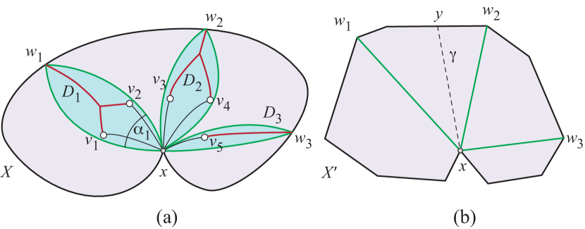
We extend the notion of star unfolding to be based on a quasigeodesic loop rather than on a point. This gives a new general method to unfold the surface of any convex polyhedron to a simple (non-overlapping), planar polygon: cut along one shortest path from each vertex of to , and cut all but one segment of .
1 Introduction
There are two general methods known to unfold the surface of any convex polyhedron to a simple (non-overlapping) polygon in the plane: the source unfolding and the star unfolding. Both unfoldings are with respect to a point . Here we define a third general method: the star unfolding with respect to a simple closed “quasigeodesic loop” on . In a companion paper [IOV09], we extend the analysis to the source unfolding with respect to a wider class of curves .
The point source unfolding cuts the cut locus of the point : the closure of the set of all those points to which there is more than one shortest path on from . The notion of cut locus was introduced by Poincaré [Poi05] in 1905, and since then has gained an important place in global Riemannian geometry; see, e.g., [Kob67] or [Sak96]. The point source unfolding has been studied for polyhedral convex surfaces since [SS86] (where the cut locus is called the “ridge tree”).
The point star unfolding cuts the shortest paths from to every vertex of . The idea goes back to Alexandrov [Ale50, p. 181];222 It is called the “Alexandrov unfolding” in [MP08]. that it unfolds to a simple (non-overlapping) polygon was established in [AO92].
In this paper we extend the star unfolding to be based on a simple closed polygonal curve with particular properties, rather than on a single point. This unfolds any convex polyhedron to a simple polygon, answering a question raised in [DO07, p. 307].
The curves for which our star unfolding works are quasigeodesic loops, which we now define.
Geodesics & Quasigeodesics.
Let be any directed curve on a convex surface , and be any point in the relative interior of , i.e., not an endpoint. Let be the total surface angle incident to the left side of , and the angle to the right side. is a geodesic if . A quasigeodesic loosens this condition to and , again for all interior to [AZ67, p. 16] [Pog73, p. 28]. So a quasigeodesic has total face angle incident to each side at all nonvertex points (just like a geodesic), and has at most angle to each side where passes through a polyhedron vertex. A simple closed geodesic is non-self-intersecting (simple) closed curve that is a geodesic, and a simple closed quasigeodesic is a simple closed curve on that is quasigeodesic throughout its length. As all curves we consider must be simple, we will henceforth drop that prefix.
A geodesic loop is a closed curve that is geodesic everywhere except possibly at one point, and similarly a quasigeodesic loop is quasigeodesic except possibly at one point , the loop point, at which the angle conditions on and may be violated—one may be larger than . Quasigeodesic loops encompass closed geodesics and quasigeodesics, as well as geodesic loops.
Pogorelov showed that any convex polyhedron has at least three closed quasigeodesics [Pog49], extending the celebrated earlier result of Lyusternik-Schnirelmann showing the same for differentiable convex surfaces. However, there is no algorithm known that will find a simple closed quasigeodesic in polynomial time: Open Problem 24.2 [DO07, p. 374].
Fortunately it is in general easy to find quasigeodesic loops on a given : start at any nonvertex point , and extend a geodesic from in opposite directions, following each branch until a self-intersection point is found, either between branches or within one branch. If no vertices are encountered, we have a geodesic loop; if vertices are encountered, at each vertex continue in an arbitrary direction that maintains quasigeodesicity, to obtain a quasigeodesic loop. An exception to this ease of finding a quasigeodesic loop could occur on an isosceles tetrahedron: a tetrahedron whose four faces are congruent triangles, or, equivalently, one at which the total face angle incident to each vertex is . It is proved in [IV08b] that a convex surface possesses a simple quasigeodesic line—a non-self-intersecting quasigeodesic infinite in both directions—if and only if the surface is an isosceles tetrahedron.
Discrete Curvature.
The discrete curvature at any point is the angle deficit or gap: minus the sum of the face angles incident to . The curvature is only nonzero at vertices of ; at each vertex it is positive because is convex. By the Gauss-Bonnet theorem, a closed geodesic partitions the curvature into in each “hemisphere” of . For quasigeodesics that pass through vertices, the curvature in each half is at most . The curvature in each half defined by a quasigeodesic loop depends on the angle at the loop point.
Some Notation.
For a quasigeodesic loop on , separates into two “halves” and . As our main focus is usually on one such half, to ease notation we sometimes use without a subscript to represent either of or when the distinction between them does not matter. Unless otherwise stated, vertices of are labeled in arbitrary order. We will use to denote a shortest path on between and . Other notation will be introduced as needed.
2 Examples and Algorithm
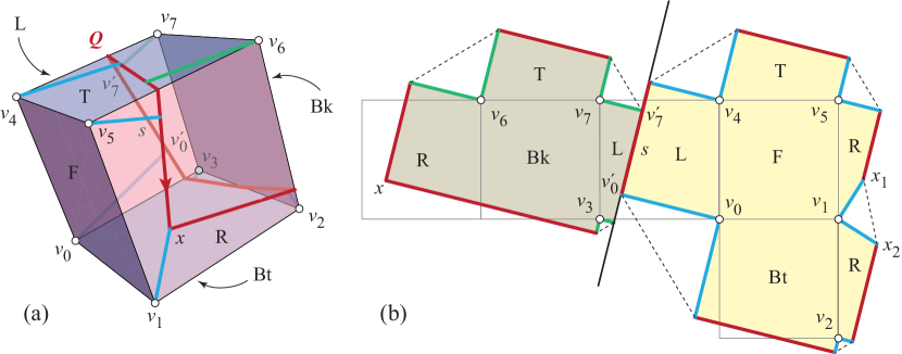
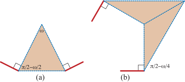
We start with an example. Figure 1(a) shows a geodesic loop on the surface of a cube. at every point of except at , where and . Note that three cube vertices, are to the left of , and the other five to the right. This is consistent with the Gauss-Bonnet theorem, because has a total turn of , so turn plus enclosed curvature is .
For each vertex , we select a shortest path to : a geodesic from to a point whose length is minimal among all geodesics to . In general there could be several shortest paths from to ; we use to represent an arbitrarily selected one. The point is called a projection of onto . In this example, for each there is a unique shortest path , which is the generic situation.
Algorithm.
If we view the star unfolding as an algorithm with inputs and , it consists of three main steps:
-
1.
Select shortest paths from each to .
-
2.
Cut along all and flatten each half.
-
3.
Cut along , joining the two halves at an uncut segment .
After cutting along , we conceptually insert an isosceles triangle with apex angle at each , which flattens each resulting half. One half (in our example, the left half), is convex, while the other resulting half may have several points of nonconvexity, at the images of . (In our example, only the image is nonconvex, when the inserted “curvature triangles” are included.) In the third and final step of the procedure, we select a segment of whose interior contains neither a vertex nor any vertex projection , such that the extension of is a supporting line of each half, and cut all of except for . In our first example, we choose (many choices for work in this example), which leads to non-overlap of the two halves.
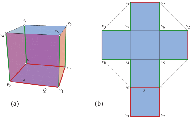
We illustrate with one more example before proceeding. Again is a cube, but now is the closed quasigeodesic composed of the edges bounding one square face, the bottom face in Figure 2(a). Cutting four shortest paths from the other vertices orthogonal to , and cutting all but one edge of , results in the standard Latin-cross unfolding of the cube shown in (b).
We now proceed to detail the three steps of the procedure, this time with proofs. Because the proofs for quasigeodesics are straightforward in comparison to the proofs for quasigeodesic loops, we separate the two in the exposition.
3 Quasigeodesics
3.1 Shortest Path Cuts for Quasigeodesics
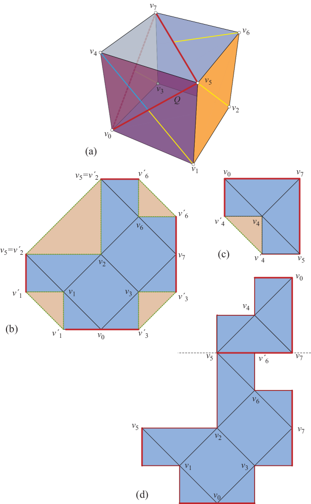
We again use a cube as an illustrative example, but this time with a closed quasigeodesic , not a loop: ; see Figure 3(a). There is angle incident to the right at , and incident to the left; and similarly at and . At all other points , . Thus is indeed a quasigeodesic. We will call the right half (including ) , and the left half (including ) . In Figure 3(a), the paths from are uniquely shortest. From there are three paths tied for shortest, and from also three are tied.
A central fact that enables our construction is this key lemma from [IIV07, Cor. 1], slightly modified for our circumstances:
Lemma 1
Let be a simple closed polygonal curve on a convex surface , and let be any point of one (closed) half-surface bounded by , but not on . Let be one of the points of closest to . Then for any choice of , the angle made by with at is at least . In particular, if is not a corner of then and the path is unique as shortest between and , and occurs only at corners where the angle of toward is larger than .
A second fact we need concerning the shortest paths is that they are disjoint.
Lemma 2
Any two shortest paths and are disjoint, for distinct vertices .
Proof: Suppose for contradiction that at least one point is shared: . We consider four cases: one shortest path is a subset of the other, the shortest paths cross, the shortest paths touch at an interior point but do not cross, or their endpoints coincide.
-
1.
. Then contains a vertex in its interior, which violates a property of shortest paths [SS86, Lem. 4.1].
-
2.
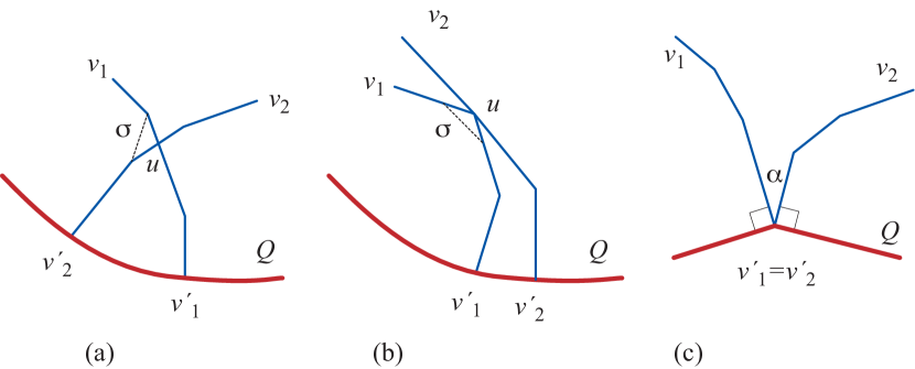
and cross properly at . It must be that , otherwise both paths would follow whichever tail is shorter. But now it is possible to shortcut the path in the vicinity of via as shown in Figure 4(a), and the path is shorter than .
-
3.
and touch at but do not cross properly there. Then there is a shortcut to one side (the side with angle less than ), as shown in Figure 4(b).
-
4.
. From Lemma 1 we know the two paths are orthogonal to the quasigeodesic at hence, since they cannot be in the situation of Case 1, there is an angle separating the paths in a neighborhood of the common endpoint; see Figure 4(c). Then has more than angle to one side at this point, violating the definition of a quasigeodesic.
This lemma ensures that the cuttings along do not interfere with one another.
3.2 Flattening the Halves for Quasigeodesics
The next step is to flatten each chosen half and (independently) by suturing in “curvature triangles” along each path. Let be one of or . The basic idea goes back to Alexandrov [Ale05, p. 241, Fig. 103], and was used also in [IV08a]. Let be the length of a shortest path , and let be the curvature at . We glue into the isosceles curvature triangle with apex angle gluing to , and incident sides of length gluing along the cut . This is illustrated in Figure 3(b,c). We display this in the plane for convenience of presentation; the triangle insertion should be viewed as operations on the manifolds and , each independently.
This procedure only works if , for becomes the apex of the inserted triangle . If , we glue in two triangles of apex angle , both with their apexes at .333 One can view this as having two vertices with half the curvature collocated at . Slightly abusing notation, we use to represent these two triangles together. In fact we must have for any vertex (else there would be no face angle at ), so and this insertion is indeed well defined.
We should remark that an alternative method of handling would be to simply not glue in anything to the vertex with , in which case we still obtain the lemma below leading to the exact same unfolding.
Now, because is the curvature (angle deficit) at , gluing in there flattens to have total incident angle . Thus is no longer a vertex of (and two new vertices are created along the bounding curve).
Let be the new manifold with boundary obtained after insertion of all curvature triangles into . We claim that a planar development of does not overlap; i.e., is isometric to a simple planar polygonal domain.
In the proof we use two results of Alexandrov. The first is his celebrated theorem [Ale05, Thm. 1, p. 100] that gluing polygons to form a topological sphere in such a way that at most angle is glued at any point, results in a unique convex polyhedron.
The second is a tool that relies on this theorem:
Lemma 3
Let be a polyhedral manifold with convex boundary, i.e., the angle towards of the left and right tangent directions to is at most at every point. Then the closed manifold obtained by gluing two copies of along is isometric to a unique polyhedron, with a plane of symmetry containing , which is a convex polygon in .
Proof: That is a convex polyhedron follows from Alexandrov’s gluing theorem. Because has intrinsic symmetry, a lemma of Alexandrov [Ale05, p. 214] applies to show that the polyhedron has a symmetry plane containing the polygon .
Now we apply these lemmas to :
Lemma 4
For each half of , is a planar convex polygon, and therefore simple (non-overlapping).
Proof: is clearly a topological disk: is, and the insertions of ’s maintains it a disk. At every interior point of , the curvature is zero by construction. So the interior is flat.
Next we show that the boundary is convex. This follows from the orthogonality of guaranteed by Lemma 1, as the base angle of the inserted triangle(s) is for , or for (see Figure 5; ), so the new angle is smaller than by or .
Now we know that is homeomorphic to a disk, and it has a convex boundary . We next prove it is isometric to a planar convex polygon by applying Lemma 3. Let be the result of gluing two copies of back-to-back along . The lemma says that has a symmetry plane containing . As all the vertices of are on , itself must be planar (and doubly covered). Therefore is a planar convex polygon, and therefore simple.
Note that, when the total curvature in is then the straight development of is turned by the insertions, as in Figure 3(b). When the total curvature in is less than , the development of is not straight, but the insertions turn it exactly the additional amount needed to close it to , as in (c) of the same figure.
3.3 Joining the Halves for Quasigeodesics
The third and final step of the unfolding procedure selects a supporting segment whose relative interior does not contain a projection of a vertex. All of will be cut except for . When is a closed quasigeodesic, any choice for generates a supporting line to a planar development of , , because is a convex domain. Then joining planar developments of and along places them on opposite sides of the line through , thus guaranteeing non-overlap. See Figure 3(d), where .
4 Quasigeodesic Loops
We now turn to the case when is a closed quasigeodesic loop with loop point , at which the angle toward is . See Figure 1, where .
4.1 Shortest Path Cuts for Quasigeodesic Loops
Lemma 1, claiming that the shortest path is unique and orthogonal to at , needs no modification. For , the shortest path makes a non-acute () angle with on both sides. Lemma 2, claiming disjointness of the shortest paths for distinct vertices , need only be modified by observing that more than one shortest path can project to , but the paths do not intersect other than at . The proof is identical.
The significant differences between quasigeodesics and quasigeodesic loops are concentrated largely in the proof for flattening, and in the proof for joining the halves. We should emphasize that the three algorithm steps detailed earlier are the same; it is only the justification that becomes more complicated.
4.2 Flattening the Halves for Quasigeodesic Loops
We aim to prove the analog of Lemma 4 for quasigeodesic loops: is (isometric to) a simple, planar polygon. Obviously that lemma establishes this for the convex half of . Let be the nonconvex half, in which the angle at exceeds .
The argument will be different (and easier) if no vertices project to .
4.2.1 No Vertex Projects to
Lemma 5
If no vertex of projects to , then is a simple, planar polygon.
Proof: Let be a geodesic on bisecting the angle at , and meeting at ; see Figure 6.
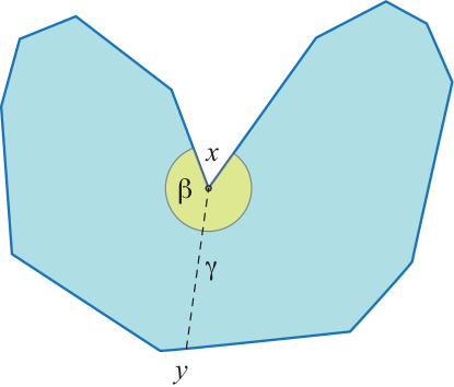
Because is flat, does in fact meet the boundary of , i.e., it does not self-cross before reaching the boundary. Cut along into two manifolds. Because , the angle at in each manifold is less than . Therefore, we have obtained exactly the situation in Lemma 4: each is a flat manifold homeomorphic to a disk, with a convex boundary. Each is therefore isometric to a planar convex polygon, with a supporting line through . Therefore they may rejoin along to form a planar simple polygon, with one reflex (concave) vertex at .
4.2.2 Vertices project to
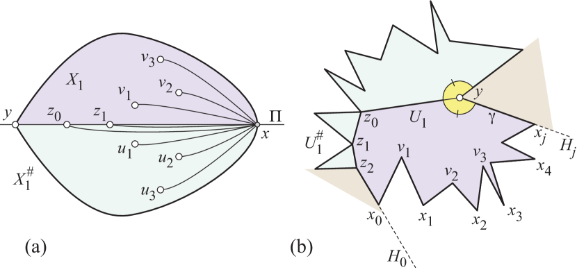
Now we consider the more difficult case, when vertices in a set project to . Rather than construct directly as above, we proceed in two stages: first we insert curvature triangles for all those vertices of that project to , forming a (nonflat) manifold , and then argue that unfolds without overlap. We will not insert curvature triangles for the vertices in , but rather argue directly for non-overlap of a flattening of . The boundary of will consist of two portions: a convex chain deriving from and the insertion of the curvature triangles, and a nonconvex chain deriving from and the vertices . Much as in Figure 6, we will cut by a geodesic and later glue the two unfolding pieces back along . We will see that the chain is formed of subchains of particular star unfoldings with respect to .
Preliminaries.
We need several ingredients for this proof. First, we will need the cut locus of on the manifold-with-boundary , which may be defined as in Section 1: is the closure of the set of all points of joined to the source point by at least two shortest paths on .
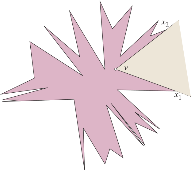
Second, we need two extensions to the theorem established in [AO92, Thm. 9.1] that the star unfolding of a polyhedron does not overlap. That paper assumed the source point was generic in the sense that it had a unique path to every vertex. We extend the result to the case when has two or more distinct shortest paths to a vertex : then simply cutting one of the paths to again leads to non-overlap. The second extension is more substantive. For any three points in the plane, forming the counterclockwise angle at , define the wedge determined by these points to be the set of points such that the segment falls within the angle : counterclockwise of and clockwise of . So the wedge is an angle apexed at when , and the complement of an angle when .
Lemma 6
Let be a vertex of the star unfolding of a polyhedral convex surface with respect to , and and the images of resulting from cutting a shortest path . Then is disjoint from the open wedge determined by , or, equivalently, is enclosed in the closed wedge determined by .
See Figure 7.
We will also need this fact:
Lemma 7
Let be a convex polyhedron obtained by doubling as in Lemma 3. Then a shortest path from a vertex on the symmetry plane , to a vertex not on , lies completely in the half containing .
Proof: Let be in the bottom half. Suppose for contradiction that a shortest path includes a section that enters the top half at and exits back to the bottom half at . Then we can reflect through to place it on the bottom half, without changing its length. Because shortest paths on convex surfaces do not branch, we obtain a contradiction.
The flattening proof consists of two parts: first, a procedure is used to find the splitting geodesic , or to determine no such geodesic exists. The second part then has two cases for reaching the final unfolding.
Part I: Excising Digons.
We now describe a process to flatten a subset of by cutting out regions containing all its interior vertices. The flattened version will then be used in further steps of the proof.
Recall we defined as the manifold obtained by inserting curvature triangles into for all shortest paths incident to , but leaving unaltered. So is not flat, but its boundary is the simple closed convex curve .
Let be the cut locus of on . In general is a forest of trees, each of which meets in a single point, and whose leaves are the vertices in . This follows from the proof of Theorem A in [ST96], but may also be seen intuitively as follows. A remark of Alexandrov [Ale05, p. 236] shows that may be extended to a convex polyhedral surface . The cut locus of on is a tree, which gets clipped by to a forest on . Another way to see this is to observe that, at every vertex interior to , a geodesic edge of emanates, and when two such edges meet interior to , they join to start a third edge of .
Let be the points of . Each is joined to by at least two shortest paths, and the union of two of these bounds a digon that includes the tree component of incident to .
Cut out from all ’s, and glue back their boundary segments in to get a new surface . Because the vertices of have been excised with the digons, is flat. And is convex except (possibly) at . Therefore, the argument of Lemma 5 applies to , showing that it is the join of two planar convex polygons.
We illustrate this construction before proceeding with the proof, first with a real example, second with an abstract example. Figure 8(a) illustrates for the geodesic loop on a cube from Figure 1; only projects to . is in this case the single segment . After excising the digon bound by the two shortest paths, the planar polygon shown in (b) is attained.
A more generic situation is illustrated in Figure 9.
Part II: Partitioning , Case 1.
The next step of the proof is to partition the manifold into pieces each of which has a convex boundary. The partition will be into either two or three pieces. We start with the two-piece Case 1. Let be the digon angle of at on . Then the angle at on is reduced by on . Case 1 holds when there is a segment on from to some point such that the corresponding geodesic on splits the angle at into two parts, each of which is at most . (It is not possible to simply select the bisector of on for , because that bisector might fall inside the of one of the digons, and so not be realized in .) Assuming for Case 1 that such a exists, we partition by cutting along , resulting in two (nonflat) manifolds and . Note that each such manifold has a convex boundary: is convex at every point excepting , the angle at is less than , and we have conveniently split the angle at . Therefore, we may apply the “doubling” Lemma 3 to each half. Henceforth we fix our attention to .
According to that lemma, we have a convex polyhedron with lying in the symmetry plane . We’ll call the portion above and below the upper and lower halves respectively. The upper half includes (a subset of) vertices of , say , and the lower half includes equivalent copies, call them . There are a number of vertices on deriving from , including , ; call them , with adjacent to .
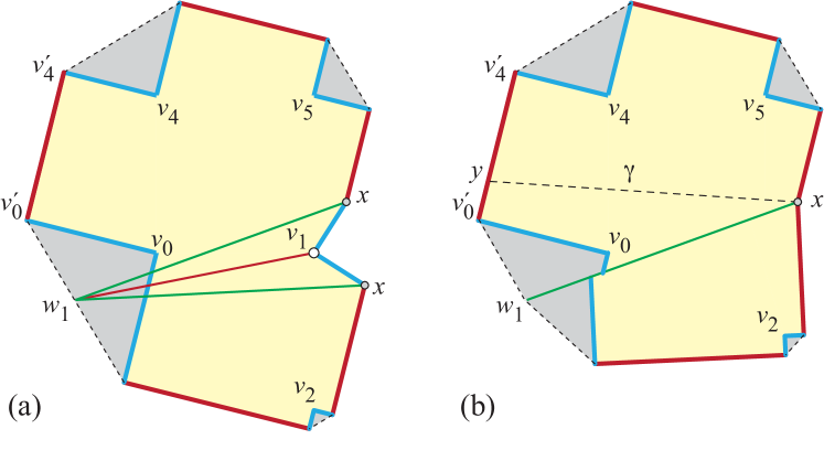
Now the plan is to construct the star unfolding of with respect to the point . By Lemma 7, the shortest paths from to the vertices of in lie wholly in one half or the other. For a vertex on , either the shortest path lies in , or there are pairs of equal-length shortest paths, one in the upper and one in the lower half. By our extension of the star unfolding theorem, we may choose which shortest path to cut in the case of ties, and still obtain a non-overlapping unfolding. We choose to select all shortest paths to the vertices on in the lower half (or along if that is where they lie). See Figure 10(a). Note that will necessarily lie in , and it is also necessarily a shortest path from to (because it is an edge of the polyhedron, and every edge of a polyhedron is a shortest path between its endpoints). So we cut as well. The result is a planar, non-overlapping unfolding . Now, identify within the portion corresponding to the upper half. Also note that is one edge of . Let and be the images of adjacent to . See Figure 10(b). Note that is a subchain of the nonconvex chain mentioned earlier, and its complementary chain in is a subchain of the convex chain .
Next we perform the exact same procedure for , resulting in containing . Now glue to along their boundary edges deriving from . Applying Lemma 6 at the point in each unfolding shows that they join without overlap, as follows.

Let be the angle at in , and the angle in . If coincides with a vertex of , then , hence joining the closed wedges enclosing and leaves at an empty open wedge of measure . If is not a vertex of , then , hence the closed wedges enclosing and are complementary; see Figure 11. Thus, in either case, the contained and do not overlap one another. And so we have established that is a planar simple polygon.
Part II: Partitioning , Case 2.
Case 1 relies on the existence of a segment on such that the corresponding geodesic on splits the angle at into two parts, each of which is at most . Now we consider the possibility that there is no such . We illustrate this possibility with an example before handling this case.
In Figure 12, is a tetrahedron with three right angles incident to . The geodesic loop shown has at an angle in the lower half, and two vertices and , included in the same digon, projecting to . In this example, the sole digon constitutes the majority of ,
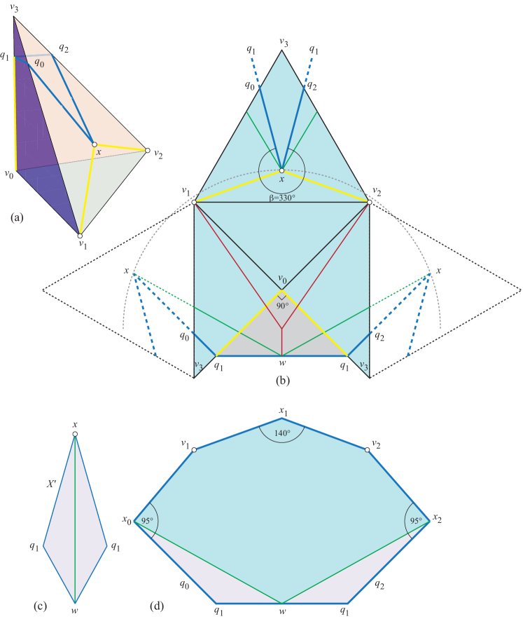
and its removal leaves ((c) of the figure) so narrow as to not admit a with the desired angle-splitting properties.
In this case, we have a “fat” digon (possibly ) whose angle at covers all the possible splitting segments . Let to ease notation, and let and be the two boundary edges (shortest paths) of connecting to . Let and be the vertices adjacent to on . The angle from to , and the angle from to , are both less than . Now we define three (topologically) closed submanifolds of : , the portion bounded by and containing vertex , , the portion bounded by and containing vertex , and the digon in between. and have convex boundaries, just as the manifolds in Case 1, and we go through the identical process:
The digon might not be convex at ; in Figure 12(a) the angle at is . So we cannot use the doubling lemma. Instead we glue (“zip”) to , which produces a convex polyhedron containing the vertices of inside , and vertices at and at . Now we produce the star unfolding of with respect to . Note that is a shortest path on , so that gets cut as part of the star unfolding. Call this unfolding . By Lemma 6, is contained within the closed wedge at , with wedge rays along and .
Finally, we join to along , and to along , nonoverlapping by the wedge properties, and conclude that the contained is a planar simple polygon. See Figure 12(d).
Finally, removing the inserted curvature triangles from establishes the analog of Lemma 4:
Lemma 8
For a quasigeodesic loop, the star unfolding of the nonconvex half of is a planar, simple polygon.
4.3 Joining the Halves for Quasigeodesic Loops
Let be the edge of the unfolding on which lies (in Case 1) or on which lies (in Case 2). If or is at a vertex of , then let be either incident edge. We claim that the line containing is a supporting line to . We establish this by identifying a larger class of supporting lines, which includes . We make the argument for Part II, Case 1 above (when exists), as Case 2 is very similar.
Returning to Figure 10(b), consider the two empty wedges exterior to , incident to the vertex adjacent to that is not ( in that figure), and the vertex adjacent to that is not , i.e., . Let and be the halflines on those wedge boundaries that include and respectively. The empty wedges imply that is included in the convex region of the plane delimited by , , and the convex boundary : the nonconvex boundary portion can cross neither nor . Let be the point , which might be “at infinity” if those halflines diverge. Similarly, is included in a region delimited by and , which meet at or not at all if those halflines diverge. Let be the line containing , which contains , and and when those exist. We consider three cases.
-
1.
Both and exist. See Figure 13(a). Then there are two supporting lines parallel to , and every edge between them along is supporting to and so to .
-
2.
exists, but does not. See Figure 13(b). We have the one line parallel to supporting . Let be the point on on the opposite side of from that maximizes the chain of visible from . Then again every edge between the two supporting lines is supporting to and so to .
-
3.
Neither nor exist. See Figure 13(c). Then again let be the point on on the opposite side of that maximizes the visibility of . Then all the edges between the tangency points extend to supporting line.
In particular, we see that the line(s) extending edge(s) incident to are among the supporting lines, as claimed.

One issue remains. It could be that the segment identified above is the base of a curvature triangle, rather than a segment of , in which case it cannot be used for joining the halves. Returning to Figure 5, there are two cases: (a) , and (b) . In case (a), is the base of a curvature triangle, with the angle at either endpoint of the base larger than . Note that edges adjacent to must be edges of . Regardless of the angle at which intersects , one of these two adjacent edges must include supporting portion of , for example, visible from in Figure 13(b,c). In case (b), two curvature triangles are inserted, but as we noted earlier, neither is truly needed, for the boundary of ( in Lemma 4) is already convex at the apexes of the two curvature triangles. So, simply not inserting them leaves an edge of crossed by that can serve as . So, in all situations, we obtain a supporting segment.
5 Conclusion
We have established our main theorem:
Theorem 1
Let be a quasigeodesic loop on a convex polyhedral surface . Cutting shortest paths from every vertex to , and cutting all but a supporting segment of as designated above, unfolds to a simple planar polygon.
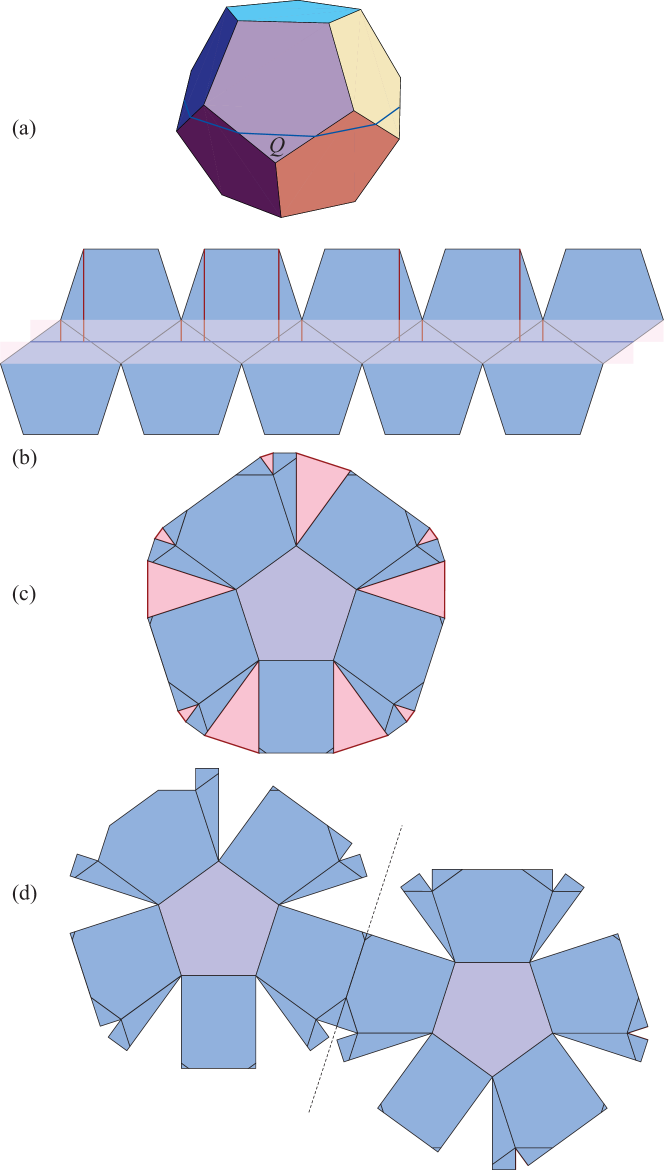
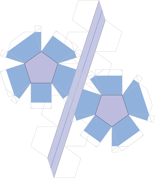
Figure 14 shows another example, a closed geodesic on a dodecahedron, this time a pure geodesic. The unfolding following the above construction is shown in Figure 14(c,d). In this case when is a pure, closed geodesic, there is additional structure that can be used for an alternative unfolding. For now lives on a region isometric to a right circular cylinder. Figure 14(b) illustrates that the upper and lower rims of the cylinder are loops parallel to through the vertices of at minimum distance to (at least one vertex on each side.) In the figure, these shortest distances to the upper rim are the short vertical paths from to the five pentagon vertices. Those rim loops are themselves closed quasigeodesics. An alternative unfolding keeps the cylinder between the rim loops intact and attaches the two reduced halves to either side. See Figure 15.
5.1 Future Work
We have focused on establishing Theorem 1 rather than the algorithmic aspects. Here we sketch preliminary thoughts on computational complexity. Let be the number of vertices of , and let be the number of faces crossed by the geodesic loop . In general cannot be bound as a function of . Let be the total combinatorial complexity of the “input” to the algorithm. Constructing from a given point and direction will take time. Identifying a supporting segment , and laying out the final unfolding, is proportional to . The most interesting algorithmic challenge is to find the shortest paths from each vertex to . The recent linear-time algorithm in [SS08] leads us to expect the computation can be accomplished efficiently.
We do not believe that quasigeodesic loops constitutes the widest class of curves for which the star unfolding leads to non-overlap. Extending Theorem 1 to quasigeodesics with two exceptional points, one with angle larger than to one side, and the other with angle larger than to the other side, is a natural next step, not yet completed.
If one fixes a nonvertex point and a surface direction at , a quasigeodesic loop can be generated to have direction at . It might be interesting to study the continuum of star unfoldings generated by spinning around .
Acknowledgments.
We thank Boris Aronov for many observations and suggestions which improved the paper.
References
- [Ale50] Aleksandr Danilovich Alexandrov. Vupyklue Mnogogranniki. Gosydarstvennoe Izdatelstvo Tehno-Teoreticheskoi Literaturu, 1950. In Russian. See [Ale58] for German translation, and [Ale05] for English translation.
- [Ale58] Aleksandr D. Alexandrov. Konvexe Polyeder. Akademie Verlag, Berlin, 1958. Math. Lehrbucher und Monographien. Translation of the 1950 Russian edition.
- [Ale05] Aleksandr D. Alexandrov. Convex Polyhedra. Springer-Verlag, Berlin, 2005. Monographs in Mathematics. Translation of the 1950 Russian edition by N. S. Dairbekov, S. S. Kutateladze, and A. B. Sossinsky.
- [AO92] Boris Aronov and Joseph O’Rourke. Nonoverlap of the star unfolding. Discrete Comput. Geom., 8:219–250, 1992.
- [AZ67] Aleksandr D. Alexandrov and Victor A. Zalgaller. Intrinsic Geometry of Surfaces. American Mathematical Society, Providence, RI, 1967.
- [DO07] Erik D. Demaine and Joseph O’Rourke. Geometric Folding Algorithms: Linkages, Origami, Polyhedra. Cambridge University Press, July 2007. http://www.gfalop.org.
- [IIV07] Kouki Ieiri, Jin-ichi Itoh, and Costin Vîlcu. Quasigeodesics and farthest points on convex surfaces. Submitted, 2007.
- [IOV07a] Jin-ichi Itoh, Joseph O’Rourke, and Costin Vîlcu. Unfolding convex polyhedra via quasigeodesics. Technical Report 085, Smith College, July 2007. arXiv:0707.4258v2 [cs.CG].
- [IOV07b] Jin-ichi Itoh, Joseph O’Rourke, and Costin Vîlcu. Unfolding convex polyhedra via quasigeodesics: Abstract. In Proc. 17th Annu. Fall Workshop Comput. Comb. Geom., November 2007.
- [IOV09] Jin-ichi Itoh, Joseph O’Rourke, and Costin Vîlcu. Source unfoldings of convex polyhedra with respect to certain closed polygonal curves. In Proc. 25th European Workshop Comput. Geom., pages 61–64. EuroCG, March 2009.
- [IV08a] Jin-ichi Itoh and Costin Vîlcu. Criteria for farthest points on convex surfaces. Mathematische Nachrichten, to appear, 2008.
- [IV08b] Jin-ichi Itoh and Costin Vîlcu. Geodesic characterizations of isosceles tetrahedra. Preprint, 2008.
- [Kob67] Shoschichi Kobayashi. On conjugate and cut loci. In S. S. Chern, editor, Studies in Global Geometry and Analysis, pages 96–122. Mathematical Association of America, 1967.
- [MP08] Ezra Miller and Igor Pak. Metric combinatorics of convex polyhedra: Cut loci and nonoverlapping unfoldings. Discrete Comput. Geom., 39:339–388, 2008.
- [OV09] Joseph O’Rourke and Costin Vîlcu. A new proof for star unfoldings of convex polyhedra. Manuscript in preparation, 2009.
- [Pog49] Aleksei V. Pogorelov. Quasi-geodesic lines on a convex surface. Mat. Sb., 25(62):275–306, 1949. English transl., Amer. Math. Soc. Transl. 74, 1952.
- [Pog73] Aleksei V. Pogorelov. Extrinsic Geometry of Convex Surfaces, volume 35 of Translations of Mathematical Monographs. American Mathematical Society, Providence, RI, 1973.
- [Poi05] Henri Poincaré. Sur les lignes géodésiques des surfaces convexes. Trans. Amer. Math. Soc., 6:237–274, 1905.
- [Sak96] Takashi Sakai. Riemannian Geometry. Translation of Mathematical Monographs 149. Amer. Math. Soc., 1996.
- [SS86] Micha Sharir and Amir Schorr. On shortest paths in polyhedral spaces. SIAM J. Comput., 15:193–215, 1986.
- [SS08] Yevgeny Schreiber and Micha Sharir. An optimal-time algorithm for shortest paths on a convex polytope in three dimensions. Discrete & Comput. Geom., 39:500–579, 2008.
- [ST96] Katsuhiro Shiohama and Minoru Tanaka. Cut loci and distance spheres on alexandrov surfaces. Séminaires & Congrès, 1:531–559, 1996. Actes de la Table Ronde de Géométrie Différentielle (Luminy, 1992).