Distinguishing cancerous from non-cancerous
cells through analysis of electrical noise

Abstract

Since 1984, electric cell-substrate impedance sensing (ECIS) has been used to monitor cell behavior in tissue culture and has proven sensitive to cell morphological changes and cell motility. We have taken ECIS measurements on several cultures of non-cancerous (HOSE) and cancerous (SKOV) human ovarian surface epithelial cells. By analyzing the noise in real and imaginary electrical impedance, we demonstrate that it is possible to distinguish the two cell types purely from signatures of their electrical noise. Our measures include power-spectral exponents, Hurst and detrended fluctuation analysis, and estimates of correlation time; principal-component analysis combines all the measures. The noise from both cancerous and non-cancerous cultures shows correlations on many time scales, but these correlations are stronger for the non-cancerous cells.

I INTRODUCTION

Electrical cell-substrate impedance sensing (ECIS) has been in use since 1984 Giaever and Keese (1984) to monitor changes in cell cultures due to spreading or in response to chemical stimuli, infection, or flow. Applications include studies of cell migration, barrier function, toxicology, angiogenesis, and apoptosis. Several papers have noted that impedance fluctuations are associated with cellular micromotion Luong (2003). However, we are not aware of any previous work applying statistical techniques to these fluctuations in order to distinguish two different cell types. Here, we demonstrate that measures of the electrical noise from cultures of cancerous and non-cancerous human ovarian surface epithelial cells distinguish them. We find that the noise in both cancerous and non-cancerous cultures shows correlations on many time scales, but by all measures, these correlations are weaker or of shorter range in the cancerous cultures.

II Experimental Methods

We used the ECIS system to collect micro-motion time-series data, the fluctuations in which are caused by the movements in a confluent layer of live cells. The system can be modeled as an RC circuit Giaever and Keese (1989, 1991); Lo et al. (1993, 1995). The cells are cultured on a small gold electrode $(5\times 10^{-4}\,{\rm cm}^{2})$, which is connected in series to a 1-Megaohm resister, an AC signal generator operating at 1 volt and 4000 Hz, and finally to a large gold counter-electrode $(0.15\,{\rm cm}^{2})$. This network is connected in parallel to a lock-in amplifier, and the in-phase and out-of-phase voltages are collected once a second, from which we extract time series of resistance and capacitive reactance (Figure 1a). In ECIS experiments, the fluctuations in complex impedance come primarily from changes in intercellular gaps and in the narrow spaces between the cells and the small gold electrode Giaever and Keese (1991); Lo et al. (1995, 1993). A current of about one microamp is driven through the sample, and the resulting voltage drop of a few millivolts across the cell layer has no physiological effect: this is a noninvasive, in vitro-technique. An ovarian cancer line (SKOV3) and a normal human ovarian surface epithelial (HOSE) cell line (HOSE15) were provided by Dr. Samuel Mok at Harvard Medical School. These cells were grown in M199 and MCDB 105 (1:1) (Sigma, St. Louis, MO) supplemented with 10% fetal calf serum (Sigma), 2mM L-glutamine, 100 units/ml penicillin, and 100 microgram/ml streptomycin under 5% CO₂, and a 37${}^{\circ}\,$C, high-humidity atmosphere. For ECIS micro-motion measurements, cells were taken from slightly sub-confluent cultures 48 hours after passage, and a mono-disperse cell suspension was prepared using standard tissue-culture techniques with trypsin/EDTA. These suspensions were equilibrated at incubator conditions before addition to the ECIS electrode wells. Confluent layers were formed 24 hours after inoculation, resulting in a density of $10^{5}{\rm cell}/{\rm cm}^{2}$.

Figure 1: Scheme of data extraction from noise. (a) Time series of resistance for one of the experimental runs. Taking the discrete time derivative and normalizing to zero mean and unit variance gives the noise, (b). The power spectrum of noise is shown in (c), using overlapping windows of 256 points in order to reduce scatter. Fits to the first hundred and last hundred frequencies estimate low- and high-frequency power-laws, $f^{-\alpha}$. White noise would have appeared frequency-independent ($\alpha=0$). The Fourier transform of the power spectrum gives the autocorrelation, (d), which we fit to a shifted power-law decay and extract the measure $\beta_{0}$. As explained in the text, subtle differences in the univariate noise distribution (e) (smoothed) discriminate between cancerous and non-cancerous micromotion.

Figure 1a shows a representative 4096-second run (just over one hour) measuring the real part of impedance as a function of time; the example shows a HOSE culture, but to the eye, SKOV cultures do not appear very different. While the example shows increasing resistance with time, others show a decrease; at this time scale, there is no evidence for an overall trend. We collected, under similar conditions, 18 time series for HOSE cultures, of which 16 went for 8192 seconds and two for 4096 seconds. Each 8192-second run was split in two halves, so that effectively we had thirty-four 4096-second runs; however, where appropriate in the analysis below, we discard the second halves of the longer runs in order to avoid inadvertently introducing correlations. Similarly, for SKOV cultures we took data in eight 8192-second runs and ten 4096-second runs, yielding effectively twenty-six 4096-second runs. We numerically differentiated the resistance and capacitance time series to obtain noise time series for each, which we normalized to zero mean and unit variance (Figure 1b).

III Statistical Measures of Noise

We seek information from the normalized noise series. The first question to pose is whether the noise can distinguish cancerous from non-cancerous cultures, but more generally the measures we extract may be used to test models of cell micromotion. Broadly, such models may be characterized by short-term and long-term correlation, so we look at several measures for each.

First, the power spectral density (Figure 1c) looks very much more like “pink noise” than “white noise;” that is, it shows signs of long-time correlations. A log-log plot of spectral density against frequency, $f$, suggests an intensity going as $f^{-\alpha}$ in the low-frequency limit. (We discuss below the extent to which a true white-noise process may mimic pink noise due to the finite time of a run.) For each run, we split the 4096 noise amplitudes into overlapping bins of 256 seconds, multiplied by a Hann window, Fourier transformed, and squared, averaging the resulting spectra in order to reduce scatter Press et al. (1994).

As in the example of the figure, some runs show a crossover between low- and high-frequency values for $\alpha$, which we estimated with least-squares straight-line fits of power at the first 100 (excluding zero frequency and the very lowest frequency) and last 100 frequencies. In many runs, low- and high-frequency alpha estimates were equal, within fitting errors. Table 1 summarizes the results, giving in the columns labeled “ave” the means over all HOSE runs or all SKOV runs for the given measures. The differences between alphas for HOSE and SKOV, both low- and high-frequency, exceed several standard errors (or standard deviations of the mean, std$/\sqrt{N}$, where $N$ is the number of runs). Moreover, the Student-$t$-test and Kolmogorov-Smirnov test show that the HOSE and SKOV populations differ . The low-frequency exponents are more significant. The fact that these measures are larger for HOSE than for SKOV suggests a difference in long-time correlations in micromotion and is consistent with the hypothesis that non-cancerous HOSE cells move in a more orderly manner than cancerous SKOV.

A non-zero $\alpha_{\rm low}$ is indicative of long-time, “fractal” Bassingthwaighte et al. (1994), correlation, but as Rangarajan and Ding Rangarajan and Ding (2000) point out, relying on power-law behavior alone can lead to incorrect identification of such correlations when none exist. Two related measures are the Hurst exponent and the exponent of detrended fluctuation analysis Mandelbrot and Wallis (1969); Bassingthwaighte et al. (1994); Feder (1988); Peng et al. (1994, 1995); Mietus et al. (2003); both methods split the time series of noise into bins of duration $T$, then determine how a measure scales with $T$. For Hurst, one subtracts the mean from all the data in a bin and characterizes that bin by its standard deviation, $S$. The series is integrated, and the minimum value subtracted from the maximum, yielding the range, $R$. For each bin, one records the ratio $R/S$ and averages over bins of the same size. The procedure is repeated for successively larger bins ($T$). A straight-line fit to a log-log plot of $R/S$ against bin size $T$ reveals a power law, $R/S\sim T^{H}$, where $H$ is the Hurst exponent. Detrended fluctuation analysis runs along similar lines, but within each bin one subtracts a best-fit line, thus detrending the data. The data in the bin are then characterized by standard deviation $S\sim T^{D}$, where $D$ is the DFA exponent. Table 2 shows the results; again, with high confidence (based particularly on Student’s $t$-test) we can conclude that HOSE and SKOV noise come from different distributions. However, since the means are separated by less than a population standard deviation, many runs (of 4096 seconds) would be necessary to determine the provenance of one particular culture.

Table 1: Power-spectral measures of HOSE (non-cancerous) and SKOV (cancerous) resistive and capacitive noise series. Shown are estimates for $1/f^{\alpha}$ behavior at high and low frequencies. The means of the alphas differ by many standard errors (std/$\sqrt{N}$), allowing us to distinguish the populations composed of $N$ runs, although not by enough to distinguish reliably a single HOSE run from a single SKOV. The $F$-test and $t$-test give the probabilities that the variances and means of the distributions of values of $\alpha$ would differ by as much as or more than they do if the two populations had come from the same Gaussian distribution. KS gives the probability under the Kolmogorov-Smirnov test that the two populations’ cumulative distributions could differ as much as they do. Small probabilities indicate that the populations differ; a probability of $0.$ means $<10^{-6}$. $N=34$ for HOSE, $N=26$ for SKOV. In all cases, we apply the approximate $t$-test for distributions with unequal variances Press et al. (1994).

	HOSE			SKOV			prob. from same distribution
measure	ave	std	std$/\sqrt{N}$	ave	std	std$/\sqrt{N}$	$F$-test	$t$-test	KS-test
resistance
$\alpha_{\rm low}$	$0.991$	$0.132$	$0.02$	$0.800$	$0.148$	$0.03$	$0.54$	$4.\times 10^{-6}$	$4.2\times 10^{-4}\hbox{\vphantom{$10^{8}$}}$
$\alpha_{\rm high}$	$1.58$	$0.558$	$0.10$	$1.09$	$0.648$	$0.13$	$0.42$	$4.\times 10^{-3}$	$0.024$
capacitance
$\alpha_{\rm low}$	$0.909$	$0.0988$	$0.02$	$0.734$	$0.131$	$0.03$	$0.13$	$0.$	$9.\times 10^{-6}\hbox{\vphantom{$10^{8}$}}$
$\alpha_{\rm high}$	$1.133$	$0.446$	$0.08$	$0.980$	$0.357$	$0.07$	$0.25$	$0.15$	$0.37$

Table 2: Additional measures of long-time correlation in the noise time series, Hurst and detrended-fluctuation exponents. See Table-1 caption for column descriptions.

	HOSE			SKOV			prob. from same distribution
measure	ave	std	std$/\sqrt{N}$	ave	std	std$/\sqrt{N}$	$F$-test	$t$-test	KS-test
resistance
Hurst $H$	$0.770$	$0.0442$	$0.008$	$0.744$	$0.0876$	$0.017$	$3.\times 10^{-4}$	$0.17$	$0.099\hbox{\vphantom{$10^{8}$}}$
DFA $D$	$0.854$	$0.0473$	$0.008$	$0.806$	$0.0793$	$0.016$	$0.006$	$9.8\times 10^{-3}$	$0.057$
capacitance
Hurst $H$	$0.792$	$0.0474$	$0.008$	$0.731$	$0.0886$	$0.017$	$9.\times 10^{-4}$	$3.1\times 10^{-3}$	$0.012\hbox{\vphantom{$10^{8}$}}$
DFA $D$	$0.843$	$0.0479$	$0.008$	$0.788$	$0.0748$	$0.015$	$0.017$	$2.5\times 10^{-3}$	$3.4\times 10^{-3}$

Table 3: Measures of short-time correlation in the noise time series: the lag at which normalized autocorrelation (see Figure 1d) falls to $1/e$, the first zero-crossing of autocorrelation, and the exponent $\beta_{0}$ from fitting the first few lags with a shifted power law. See the Table-1 caption for the statistical labels. Of these measures, the $1/e$ crossing (in resistance) and the zero crossing (in capacitance) have the greatest significance in distinguishing the populations; $\beta_{0}$ is significant only in the sense that the scatter is very much greater for cancerous SKOV than for non-cancerous HOSE.

	HOSE			SKOV			prob. from same distribution
measure	ave	std	std$/\sqrt{N}$	ave	std	std$/\sqrt{N}$	$F$-test	$t$-test	KS-test
resistance
$1/e$	$6.35$	$1.76$	$0.30$	$4.91$	$2.62$	$0.51$	$0.032$	$0.020$	$9.1\times 10^{-3}\hbox{\vphantom{$10^{8}$}}$
zero	$132.$	$88.0$	$15$	$111.$	$115.$	$23.$	$0.14$	$0.44$	$0.068$
$\beta_{0}$	$1.18$	$0.565$	$0.10$	$5.11$	$12.8$	$2.50$	$0.$	$0.13$	$0.48$
capacitance
$1/e$	$5.77$	$1.40$	$0.24$	$4.40$	$3.96$	$0.78$	$0.$	$0.10$	$6.0\times 10^{-5}\hbox{\vphantom{$10^{8}$}}$
zero	$194.$	$136.$	$23.$	$97.5$	$111.$	$22.$	$0.29$	$3.7\times 10^{-3}$	$8.6\times 10^{-3}$
$\beta_{0}$	$1.17$	$1.16$	$0.20$	$1.93$	$3.35$	$0.66$	$0.$	$0.28$	$0.71$

While $\alpha_{\rm low}$, $H$, and $D$ were designed to estimate correlations at diverging time scales, short-time correlation is conveniently determined from autocorrelation, Figure 1d, normalized to unity at zero lag. The lag of first zero crossing provides one natural measure of when correlation is lost, but since autocorrelation curves may sometimes reach very small, yet positive, plateaus before crossing zero, we also measured the lag at which the autocorrelation first crosses $1/e$. In a model with only short-time correlation, the $1/e$ time estimates the exponential decay time. However, as we discuss below, we observed significant deviations from exponential decay, finding better fits to a shifted power-law decay,

$${\rm autocorrelation}=\left({{t+t_{1}}\over{t_{1}}}\right)^{-\beta_{0}}\hbox to0.0pt{\quad.\hss}$$ (1)

We fit autocorrelation, for lags in the heuristic interval $t=1$ to $t=20$ seconds, using Levenberg-Marquardt least-squares minimization to this form to find $\beta_{0}$. Table 3 summarizes results for the two crossings and $\beta_{0}$; the last distinguishes the populations of HOSE and SKOV runs only in that (cancerous) SKOV shows much greater scatter in $\beta_{0}$, as measured by the $F$-test. Both crossings vary greatly from run to run, but the $1/e$ crossing in resistance and zero crossing in capacitance distinguish the populations of HOSE and SKOV experiments at better than the 95% confidence level as measured by Student’s $t$-test and the Kolmogorov-Smirnov test. In particular, the averaged measures show shorter crossing times and steeper descents ($\beta_{0}$) for SKOV than for HOSE, again consistent with the hypothesis that the micromotion of cancerous cultures is less correlated than that of non-cancerous cultures.

With the fourteen measures summarized in Tables 1–3, each run of 4096 seconds can be thought of as a point in a fourteen-dimensional space. In such problems, the populations might separate into two distinct, compact clusters (Lewicki, 1998, §4.2); while the identification of clusters in high-dimensional spaces remains an open problem in statistical research, it is common to use the variance-maximizing principal-component analysis introduced by Hotelling to project onto optimal subspaces, usually taken to be two-dimensional Hotelling (1933). Figure 2 plots the first two principal components. While the plot shows a clear difference between the two populations consisting of all runs of HOSE and all runs of SKOV, overlap between the two clusters makes it difficult to apply the technique diagnostically. We found this problem to be generic: an exhaustive examination of pairs of principal components (beyond the first two) produced similar plots, with the two populations usually less distinct in higher-order components, while adding or subtracting several measures to the list of fourteen measures did not improve clustering.

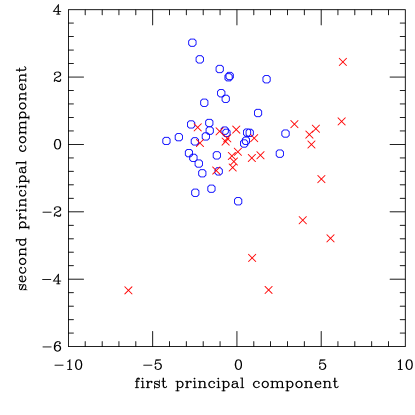
Figure 2: (Color on-line.) Projection along the first two principal components of the fourteen-dimensional space determined by Tables 1–3. Blue open symbols mark the 34 HOSE runs, red crosses the 26 SKOV experiments. As populations, these two sets are distinct, but the overlap of clusters makes it difficult to distinguish individual runs in this type of projection.

Thus far, the noise measures considered have shown that electrical noise from HOSE and SKOV experiments have, on average, different correlations, but they do not provide a reliable way to determine whether the cells in a single run of 4096 seconds are HOSE or SKOV. However, from the normalized (zero-mean, unit-variance) noise time series of Figure 1b, we can extract a probability distribution of noise amplitudes, as in Figure 1e. Not surprisingly, the distribution is approximately Gaussian; however, subtle deviations from normal form do distinguish HOSE from SKOV, even in a single run, if we apply the Kolmogorov-Smirnov test directly to the noise. This test looks only at distributions of noise amplitudes, rather than correlations.

To this end, we concatenate the first nine 4096-second HOSE resistance runs (discarding, for this purpose, the second halves of the 8192-second runs) to create a HOSE resistance reference distribution. Similarly, we create a SKOV resistance reference by concatenating the first nine 4096-second SKOV runs. Each of the remaining runs is tested against the two resistance reference sets. The same procedure is applied with capacitance data. In many cases, Kolmogorov-Smirnov does not show a match with either distribution with high probability, but we can compare the two probabilities: one typical HOSE run matches the HOSE reference with probability 0.02 and SKOV with probability $4.7\times 10^{-8}$, so we (correctly) identify this run as HOSE based on the ratio of probabilities. Of 56 tested data sets (none of which went into the construction of the reference sets), 42 (75%) matched the correct reference set by this criterion, an outcome that would happen by chance with probability approximately $1.2\times 10^{-4}$. We repeated the procedure using a second collection of four reference sets (HOSE/SKOV, resistance/capacitance) constructed from nine runs not used in making the first reference sets. Of 64 trials (none used in the new reference sets), 53 (83%) were identified correctly, with corresponding probability $5\times 10^{-8}$. The results from the two sets of trials are added and summarized in Table 4. We can reduce percentages of incorrect identifications by insisting on agreement between resistance and capacitance time series; this lowers the overall incorrect identification rate to 11.7%, with a correct rate of 70.0% and a “not-sure” rate of 18.3%.

Deviations from normality in the noise-amplitude distributions are characterized in part by kurtosis Keeping (1962), which is larger for HOSE than for SKOV: see Table 5. A possible explanation is that kurtosis here is a proxy for correlation time: since convergence under the central-limit theorem is non-uniform, with a distribution approaching a Gaussian slowly in the tails as the number of samples increases, a smaller population will tend to have a larger kurtosis than a larger one. All of our runs have the same number of time steps, but as we have seen, SKOV correlation times are shorter than HOSE correlation times; thus, a SKOV run could be said to have more independent time steps than a HOSE run of the same length and might be expected then to have a smaller kurtosis. However, this cannot explain the whole effect: as we argue in Appendix A, both kurtosis and Kolmogorov-Smirnov appear to be better discriminants than a direct measure, the $1/e$ crossing. This suggests that the univariate noise distribution is more than just a proxy for correlation time.

Table 4: Percentages of correct identifications. The Kolmogorov-Smirnov test is applied to distributions of noise amplitudes against HOSE and SKOV reference sets. Two non-overlapping choices of reference sets are used; in neither case did any trial run figure in a reference set against which it was tested. The “average” column gives percentages weighted by numbers of trials (16 HOSE and 12 SKOV in the first set, 18 HOSE and 14 SKOV in the second).

	first set	second set	average
HOSE capacitance	$62.5\hbox to0.0pt{\%\hss}$	$72.2\hbox to0.0pt{\%\hss}$	$67.6\hbox to0.0pt{\%\hss}$
HOSE resistance	$87.5$	$66.7$	$76.5$
SKOV capacitance	$83.3$	$100.$	$92.3$
SKOV resistance	$66.7$	$100.$	$84.6$
all resistance	$78.6$	$81.3$	$80.0$
all capacitance	$71.4$	$84.4$	$78.3$
all HOSE	$75.0$	$69.4$	$72.1$
all SKOV	$75.0$	$100.$	$88.5$
all	$75.0$	$82.8$	$79.2$

Table 5: Kurtosis averaged over all runs, standard deviation of kurtoses, and standard deviation of the means.

	average	std.	std./$\sqrt{N}$
HOSE resistance	$74.4$	$173.1$	$29.7$
SKOV resistance	$3.00$	$9.57$	$1.9$
HOSE capacitance	$17.6$	$32.2$	$5.5$
SKOV capacitance	$0.94$	$1.80$	$0.35$

IV TWO SIMPLE MODELS

Having motivated and interpreted our measures of noise in terms of short- and long-time correlations, we now compare our data to the simplest possible discrete-time models, the binary random walk with persistence Fürth (1920), displaying only short-time correlation, and a discrete fractional Brownian motion Mandelbrot and van Ness (1968); Rangarajan and Ding (2000), which has correlations on all time scales. For present purposes, it suffices to consider only the increments rather than the walks themselves; that is, we compare to Figure 1b, not Figure 1a.

First, consider the increments of a discrete random walk with persistence. Let the increment at time $j\Delta t$, where $\Delta t$ is the time step, be $x_{j}$, drawn from $\{+1,-1\}$. Then $x_{j+1}=x_{j}$ with probability $a$ and $x_{j+1}=-x_{j}$ with probability $1-a$; one recovers the usual discrete binary random walk for $a=1/2$. Since we think of this process as approximating a continuous one, and there is no natural way to take the limit $\Delta t\rightarrow 0$ for anticorrelated increments, we restrict $1/2\leq a\leq 1$. For convenience, we set $\Delta t=1$. A simple inductive argument shows that

$$\langle x_{0}x_{n}\rangle=(2a-1)^{n}=\exp(-n/\tau)\hbox to0.0pt{\quad,\hss}$$ (2)

where the correlation time $\tau=-1/\ln(2a-1)$. For times much larger than $\tau$, this Markov process looks like an ordinary binary random walk with a rescaled time, and by the usual arguments Reichl (1998), the power spectrum approaches white noise, i.e., it is independent of frequency. However, for a finite run, the power spectrum may mimic correlated (pink) noise even, surprisingly, for a $\tau$ as short as $4$ in a run as long as $4096$, as in Figure 3a. However, the random noise levels off noticeably at low frequencies, while the experimental data (Figure 3b) appear to follow a $1/f^{\alpha}$ power law to the lowest frequencies . This supports the presence of correlations at all time scales. The shortness of the low-frequency plateau in Figure 3a is misleading. To see more of the flat part of the spectrum, finer frequency resolution is necessary. Taking larger windows, we can (at least for a run longer than 4096) extend the graph many decades to the left and verify that the spectrum remains flat (white), but at the cost of greater scatter. Parts (c) and (d) of the figure show autocorrelation for random noise and experimental data with fits to exponential decay (dotted) and the shifted power law (1) (solid). The two fits fall on top of one another for the process satisfying (2). That exponential decay does not approximate the experimental data as well as the power law corroborates the hypothesis of longer-than-short-time correlations.

Figure 3: The increments of a finite random walk with persistence (left) may mimic certain aspects of the experimental data (right), but with notable differences. The random process has $a=0.8894$, so an exponential decay time $\tau=4.00$. The experiment is a typical capacitance noise time series of HOSE, with a measured $1/e$ crossing of $5.7$. (a) and (b) show the best-fit lines to the first 100 points (excluding zero and the lowest frequency) of the power spectrum; both give slopes $\approx-1.0$, but the random data level off noticeably at low frequencies, as would be expected of white noise. Autocorrelation curves (c) and (d) show fits to exponential (dotted line) and shifted power-law (1) (solid) decays. For the random noise, the two fits fall on top of one another, but for the experimental data, a power law fits better than exponential decay.

Mandelbrot and van Ness Mandelbrot and van Ness (1968) introduce the notion of fractional Brownian motion with correlations between increments separated by arbitrary time differences and with a $1/f^{\alpha}$ power spectrum. Rangarajan and Ding Rangarajan and Ding (2000) describe a particularly simple way of generating a time series of increments with such properties: start with a Gaussian-distributed uncorrelated time series $\{x_{j}\}$, Fourier-transform, multiply by $f^{-\alpha/2}$, and Fourier-transform back. The resulting process has a Hurst exponent given by

$$H=(1+\alpha)/2\hbox to0.0pt{\quad.\hss}$$ (3)

Determination of exponents $\alpha$ and $H$ is subject to the usual numerical vicissitudes, but Rangarajan and Ding argue that true long-ranged processes should satisfy (3) at least approximately.

Figure 4 plots fractional discrepancies between (3) and measured Hurst exponents as functions of measured spectral exponents $\alpha$. At the bottom are plotted artificially-generated long-time-correlated data following the prescription of Rangarajan and Ding (plotting symbols $+$); the measured exponents $\alpha$ are always close to the known values, so the measurement errors occur in estimating $H$. We note a systematic trend toward larger errors away from $\alpha\approx 0.5$, but generally the errors stay small. At the top of the graph (plotting symbols $\diamond$) are artificially-generated random walk increments with persistence times ranging from $2$ at the left to $7$ at the right. Measured values of $\alpha$ follow the same prescription as used above, although as noted earlier (Figure 3), the fits fail for low frequencies; indeed, every $\alpha$ should be zero. Hurst estimates range from 0.45 to 0.67; the true value in every case should be $1/2$. As discussed by Rangarajan and Ding, the discrepancies between measured Hurst and Hurst estimated from measured $\alpha$ are large. In the middle and at the bottom are plotted our experimental data (HOSE $\circ$, SKOV $\times$). Agreement between the exponents $H$ and $\alpha$ is generally not as good as for the long-range-correlated processes but not so poor as for the short-time-correlated random walk. On average, the experimental points lie closer to the former than to the latter. We interpret this result as supporting the existence of correlations on, at the very least, many different time scales. A model of cell motion will need to explain both the short-time and long-time correlations we have observed.

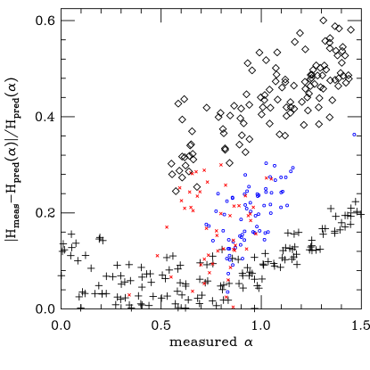
Figure 4: (Color on-line.) Fractional discrepancies between $H_{\rm pred}$ given by (3) and measured Hurst exponent as functions of measured spectral exponent $\alpha$. Near the bottom, plotted with large $+$ symbols, are artificially-generated data with known long-time correlations. At top are generated data (large $\diamond$) from random-walk increments with persistence times ranging from $2$ (smaller values of $\alpha$) to $7$ (larger values). In the middle are experimental results for HOSE (blue $\circ$) and SKOV (red $\times$). Most of the experimental data look more like the correlated data than the uncorrelated, but a few overlap with uncorrelated noise; all of these are SKOV.

V APPLICATIONS

We have demonstrated that electrical-noise measurements on human ovarian surface epithelial cells can distinguish cancerous and non-cancerous cultures. This is not intended as a diagnostic tool; for one thing, it is easier to distinguish them under a microscope. We find it is also possible to distinguish HOSE from SKOV based purely on average electrical resistance or capacitance. Our main focus has rather been on developing statistical tools with which to test more sophisticated statistical-mechanical models and in developing a database of characteristics of many different cell types, for which a single measurement (e.g., average electrical resistance) will surely be inadequate.

One characteristic of malignant cancerous cells is their ability to invade tissue in disregard of clues from their neighbors Hanahan and Weinberg (2000); our observation of shorter correlation times in cancerous cultures is consistent with the picture of cancerous cells moving in a less regulated manner. Now that it has been established that different cell types generate distinguishable noise patterns, future research in this area will focus on the development of realistic models of cellular motility for healthy and malignant cells.

Appendix A Comparing discriminators

We claim no originality to the following elementary application of statistics but could not find a textbook discussion of quite this point. Given two distributions, $A$ and $B$ (for instance, the kurtoses of HOSE data sets and those of SKOV), assumed to be Gaussian and characterized by means $\mu_{A}<\mu_{B}$ and standard deviations $\sigma_{A}$, $\sigma_{B}$, there are several choices of where to place a dividing point $x_{0}$ so as to identify all $x<x_{0}$ as belonging to population $1$ and all $x>x_{0}$ to population $2$. One natural choice is to pick $x_{0}$ so that the expected rates of correct identification of the two populations will be the same, i.e., that $x_{0}-\mu_{A}$ should be the same multiple of $\sigma_{A}$ as $\mu_{B}-x_{0}$ is of $\sigma_{B}$, or

$$x_{0}={{\mu_{A}\sigma_{B}+\mu_{B}\sigma_{A}}\over{\sigma_{A}+\sigma_{B}}}\hbox to0.0pt{\quad.\hss}$$ (4)

Any other choice will decrease the expected rate of incorrect identification of one population at the cost of increasing the other. A second plausible choice is to seek to maximize the sum of the expected correct identification rates,

$${\rm C}_{A} ={1\over 2}+{1\over 2}{\rm erf}\left({{x_{0}-\mu_{A}}\over{\sigma_{A}\sqrt{2}}}\right)$$ (5)

$${\rm C}_{B} ={1\over 2}+{1\over 2}{\rm erf}\left({{\mu_{B}-x_{0}}\over{\sigma_{B}\sqrt{2}}}\right)\hbox to0.0pt{\quad;\hss}$$

it is easy to show that the separatrix $x_{0}$ is then

$$\textstyle x_{0}\!=\!{{\mu_{B}\sigma_{A}^{2}-\sigma_{B}\left(\mu_{A}\sigma_{B}\pm\sigma_{A}\sqrt{(\mu_{A}-\mu_{B})^{2}+2(\sigma_{A}^{2}-\sigma_{B}^{2})\ln(\sigma_{A}/\sigma_{B})}\,\right)}\over{\sigma_{A}^{2}-\sigma_{B}^{2}}}\hbox to0.0pt{\quad.\hss}$$ (6)

(One root maximizes ${\rm C}_{A}+{\rm C}_{B}$. Note that (6) reduces to $(\mu_{A}+\mu_{B})/2$ when $\sigma_{A}=\sigma_{B}$.) A third natural choice, maximizing the product ${\rm C}_{A}\,{\rm C}_{B}$, requires numerical solution. Of course, a more complicated risk function could apply, for instance in medical diagnosis, where a false negative is much worse than a false positive.

To compare the predictive values of three of the statistical measures developed in the text, $1/e$ crossing from Table 3, kurtosis from Table 5, and the Kolmogorov-Smirnov test of Table 4, we apply the simplest separatrix, (4) to the means and standard deviations estimated for the first two. (This choice is motivated by the similar correct-identification percentages for HOSE and SKOV in Table 4, but as an alternative to (5), using the actual data sets gives comparable answers). Then the expected correct-identification rate (5) for $1/e$ as a discriminant is 62% and that for kurtosis 67%. These rates are both lower than the 79% (Table 4) for the Kolmogorov-Smirnov test applied to the noise distribution, undermining the idea that the deviation of this distribution from normal form is strictly a proxy for correlation time.

References

- Giaever and Keese (1984) I. Giaever and C. R. Keese, Proc. Natl. Acad. Sci. USA 81, 3761 (1984).
- Luong (2003) J. H. T. Luong, Analytical Letters 36, 3147 (2003).
- Giaever and Keese (1989) I. Giaever and C. R. Keese, Physica D 38, 128 (1989).
- Giaever and Keese (1991) I. Giaever and C. R. Keese, Proc. Natl. Acad. Sci. USA 88, 7896 (1991).
- Lo et al. (1993) C.-M. Lo, C. R. Keese, and I. Giaever, Experimental Cell Research 204, 102 (1993).
- Lo et al. (1995) C.-M. Lo, C. R. Keese, and I. Giaever, Biophysical Journal 69, 2800 (1995).
- Press et al. (1994) W. H. Press, S. A. Teukolsky, W. T. Vetterling, and B. P. Flannery, Numerical Recipes in C: the Art of Scientific Computing (Cambridge University Press, 1994), second, corrected ed.
- Bassingthwaighte et al. (1994) J. B. Bassingthwaighte, L. S. Liebovitch, and B. J. West, Fractal Physiology (Oxford University Press, New York, 1994).
- Rangarajan and Ding (2000) G. Rangarajan and M. Ding, Phys. Rev. E 61, 4991 (2000).
- Mandelbrot and Wallis (1969) B. Mandelbrot and J. Wallis, Water Resour. Res. 5, 321 (1969).
- Feder (1988) J. Feder, Fractals (Oxford University Press, New York, 1988).
- Peng et al. (1994) C.-K. Peng, S. V. Buldyrev, S. Havlin, M. Simons, H. E. Stanley, and A. L. Goldberger, Phys. Rev. E 49, 1685 (1994).
- Peng et al. (1995) C.-K. Peng, S. Havlin, H. E. Stanley, and A. L. Goldberger, Chaos 5, 82 (1995).
- Mietus et al. (2003) J. Mietus, C.-K. Peng, and G. Moody, Physio Toolkit: dfa, http://www.physionet.org/physiotools/dfa/dfa-1.htm (2003).
- Lewicki (1998) M. Lewicki, Network: Comput. Neural Syst. 9, R53 (1998).
- Hotelling (1933) H. Hotelling, J. Educ. Psych. 24, 417 (1933).
- Keeping (1962) E. Keeping, Introduction to Statistical Inference (van Nostrand (republished Dover 1995), Princeton, 1962).
- Fürth (1920) R. Fürth, Z. f. Physik 2, 244 (1920).