On the Interaction of Jupiter’s Great Red Spot and Zonal Jet Streams

Abstract

In this paper, Jupiter’s Great Red Spot (GRS) is used to determine properties of the Jovian atmosphere that cannot otherwise be found. These properties include the potential vorticity of the GRS and its neighboring jet streams, the shear imposed on the GRS by the jet streams, and the vertical entropy gradient (i.e., Rossby deformation radius). The cloud cover of the GRS, which is often used to define the GRS’s area and aspect ratio, is found to differ significantly from the region of the GRS’s potential vorticity anomaly. The westward-going jet stream to the north of the GRS and the eastward-going jet stream to its south are each found to have a large potential vorticity “jump”. The jumps have opposite sign and as a consequence of their interaction with the GRS, the shear imposed on the GRS is reduced. The east-west to north-south aspect ratio of the GRS’s potential vorticity anomaly depends on the ratio of the imposed shear to the strength of the anomaly. The aspect ratio is found to be $\approx$2:1, but without the opposing jumps it would be much greater. The GRS’s high-speed collar and quiescent interior require that the potential vorticity in the interior be approximately half that in the collar. No other persistent geophysical vortex has a significant minimum of potential vorticity in its interior and laboratory vortices with such a minimum are unstable.

Sushil Shetty, 6116 Etcheverry Hall, University of California, Berkeley, CA 94720
E-mail: sushil@newton.berkeley.edu

1 Introduction

Only a relatively thin ($\sim$10 km) outer layer of Jupiter’s atmosphere containing the visible clouds and vortices is accessible by direct observation. Most of the details of the underlying layers, such as the vertical stratification, must therefore be determined indirectly. In this paper, we present one such indirect method. In particular, we use the observed velocity field of a persistent Jovian vortex to determine quantities relevant to both outer and underlying layers. These quantities are the potential vorticity of the vortex, the potential vorticity of the neighboring jet streams, the flow in the underlying layers, and the Rossby deformation radius $L_{r}$, which is a measure of the vertical stratification. We demonstrate the method using Voyager 1 observations of the Great Red Spot (GRS).

We are not the first to use the GRS velocity field as a probe of the Jovian atmosphere (Dowling and Ingersoll, 1988, 1989; Cho et al., 2001). However, our approach differs from previous ones in several significant respects. First, the GRS velocity field is sufficiently noisy that we do not, unlike in previous analyses, take spatial derivatives of the velocity to compute potential vorticity. Instead, we solve the inverse problem: We identify several “traits” of the GRS velocity field, where a trait is a feature of the velocity field that is unambiguously quantifiable from the noisy data. We then construct a model for the flow and determine “best-fit” values for the model parameters such that the model velocity field reproduces the observed traits. Furthermore, for a given set of parameter values, we construct the model velocity field so that it is an exact steady solution of the equations that govern the flow. For the Voyager 1 data, we find that a best-fit model (i.e., a trait-reproducing steady solution) determined in this manner agrees with the entire GRS velocity field to within the observational uncertainties.

A second way in which our study differs from previous ones is that we explicitly compute the interaction between the GRS and its neighboring jet streams. We show that the interaction controls the aspect ratio of the GRS’s potential vorticity anomaly, which is relevant to recent observations that show the aspect ratio of the GRS’s cloud cover to be a function of time (Simon-Miller et al., 2002). The changing cloud cover, if symptomatic of changes in the GRS’s potential vorticity anomaly, would be indicative of a change in the interaction and a corresponding change in the best-fit values of the parameters that govern the interaction. Finally, in this study, we quantify the relationship between individual traits and individual parameters. When a trait is nearly independent of all parameters except for one or two, a clear physical understanding is obtained between “cause” (a model parameter) and ”effect” (a GRS trait).

Our philosophy is to use a model with the fewest free parameters that is an exact steady solution to the least complex governing equation, yet can still reproduce the observed velocity to within its uncertainties. The danger of more complex models is that they have larger degrees of freedom. By varying parameters they can fit the observed velocity but misidentify the relevant physics. For the Voyager 1 data considered here, we use the 1.5–layer reduced gravity quasigeostrophic (QG) equations and a model with nine free parameters. The Voyager 1 data can be reproduced with this model and does not warrant models with more free parameters or governing equations with more complexity.

The rest of the paper is organized as follows. In $\S$2 we determine the GRS velocity field from Voyager 1 observations and then identify traits of the velocity. In $\S$3 we review the governing equations and describe a decomposition of the flow around the GRS into a near-field, a far-field, and an interaction-field. In $\S$4 we define the model and list its free parameters. In $\S$5 we determine best-fit parameter values, i.e., parameter values for which the model reproduces the traits. In $\S$6 we discuss the physical implications of the best-fit model, and in $\S$7 conclude with an outline for future work.

2 GRS velocity field

2.1 Determination of GRS velocity

In Mitchell et al. (1981), Voyager 1 images were used to determine the GRS velocity field by dividing the displacement of a cloud feature in a pair of images by the time interval between the images (typically one Jovian day or $\approx$10 hours). The cloud features were identified by hand rather than by an automated approach such as Correlation-Image-Velocimetry (CIV: Fincham and Spedding 1997), and may therefore contain spurious velocities on account of misidentifications. Furthermore, dividing cloud displacement by time does not account for the curvature of a cloud trajectory, since in ten hours, a cloud feature in the high-speed collar travels almost a third of the way across the GRS. However, due to the unavailability of the original navigated images, we use the Mitchell velocities, but remove some of the errors by a procedure described in appendix A. The procedure leads to the removal of 220 of the original 1100 measured cloud displacements and the addition of 7100 synthetic measurements. The net result is that the uncertainty in the velocity field is reduced from $\approx 9$ m s^-1 to $\approx 7$ m s^-1. Fig. 1 shows the processed GRS velocity field. Consistent with previous analyses, the velocity field shows a quiescent core and high-speed collar. The inner part of the collar has anticyclonic vorticity, and the outer part has cyclonic vorticity. The peak velocities in the collar are $140\pm 7$ m s^-1 and the peak velocities in the core are $7\pm 7$ m s^-1.

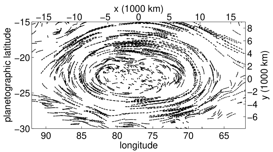
Figure 1: Velocity vectors of the GRS with respect to System III as determined from Voyager 1 images. The velocities were determined by dividing the displacement of a cloud feature in a pair of images by the time between the two images (Mitchell et al., 1981), and then correcting for the fact that cloud trajectories over typical image separation times are not straight lines (see $\S$2a). The $23^{\circ}$S latitude is defined to be the principal east-west (E–W) axis, and the $77^{\circ}$W longitude is defined to be the principal north-south (N–S) axis.

The GRS is embedded in a zonal (east-west) flow. The zonal mean of this flow, averaged over 142 Jovian days, was computed from Voyager 2 images (Limaye, 1986), and is shown in Fig. 2. Between $15^{\circ}$S and $30^{\circ}$S, the profile is characterized by a westward-going jet stream that peaks at $\approx 19.5^{\circ}$S, and an eastward-going jet stream that peaks at $\approx 26.5^{\circ}$S. The uncertainty in the profile is 7 m s^-1. (Note that most likely due to navigational errors (Limaye, 1986), the published profile must be shifted north by $0.5^{\circ}$ so as to be consistent with the navigated latitudes of Voyager 1 in Fig. 1.) The GRS was observed to drift westward at a rate of 3–4 m s^-1 with respect to System III during the Voyager epoch (Dowling and Ingersoll, 1988).

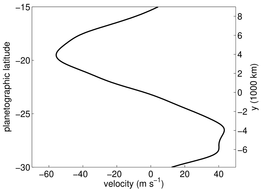
Figure 2: Averaged zonal velocity ${\bf v}^{\infty}$ in System III (Limaye, 1986).

2.2 Pitfalls to be avoided when analyzing GRS velocity

We do not compute quantities by taking spatial derivatives of the velocity data, as this tends to amplify small length scale noise. For example, in the high-speed collar, we found that the uncertainty in vorticity obtained by differentiating the velocity is $\approx 35\%$ of the maximum vorticity. If vorticities must be found, it is usually better to integrate the velocity to obtain a circulation and then divide by an area to obtain a local average vorticity. We also do not average the velocity locally, which is a standard way of reducing noise. For example, if the GRS velocity is averaged over length scales greater than $2^{\circ}$, the peak velocities and vorticities are severely diminished. This is due to the fact that an averaging length of $2^{\circ}$ is too large; it corresponds to $\approx 2500$ km, which is the length scale over which the velocity changes by order unity (cf. the width of the high-speed collar). Finally, we do not obtain a quantity by adding two numbers of similar magnitude but opposite sign, so that the resulting sum is of order or smaller than the uncertainty in each of the numbers being summed. For example, if the velocity is assumed to be divergence-free, the vertical derivative of the vertical velocity $\partial v_{z}/\partial z$ can be obtained by computing the negative of the horizontal divergence $\partial v_{x}/\partial x+\partial v_{y}/\partial y$ . However, a simple scaling argument shows that the horizontal divergence is smaller than each partial derivative term separately, and in particular, is of the same order as the uncertainty in each term (which is relatively large because the terms are derivatives of noisy data). Thus $\partial v_{z}/\partial z$ computed in this fashion would have order unity uncertainties.

2.3 Traits of GRS velocity

The traits that we consider are derived from the north-south (N–S) velocity along the principal east-west (E–W) axis and from the east-west (E–W) velocity along the principal north-south (N–S) axis. The E–W and N–S principal axes are defined to be the $23^{\circ}$S latitude and the 77^∘W longitude respectively. The point of intersection of the principal axes is roughly the centroid of the GRS as inferred from its clouds. The velocity profiles along the axes are shown in Fig. 3. To better understand the pitfalls of local averaging, Figs. 3a and 3c show the velocities from Fig. 1 for points that lie within $\pm 0.7^{\circ}$ of the axes, while Figs. 3b and 3d show the velocities that lie within $\pm 1.4^{\circ}$ of the axes. The axes labels $x$ and $y$ in the figure denote local E–W and N–S cartesian coordinates. Based on the figure, we define the following to be traits of the velocity field: (1) the northward-going jet and southward-going jet in Figs. 3(a)–(b) that peak at $x=\pm 9750\pm 500$ km respectively and have peak magnitude $V^{NS}_{\rm max}=95\pm 7$ m s^-1, (2) the small magnitude N–S velocity in $|x|\leq 6000$ km, (3) the eastward-going jet and westward-going jet in Figs. 3(c)–(d) that peak at $y=-3500\pm 500$ km and $y=5500\pm 500$ km respectively, and have peak magnitude $140\pm 7$ m s^-1, (4) the small magnitude E–W velocity in $|y|\leq 2000$ km. Traits (2) and (4) illustrate the quiescent interior of the GRS. Traits (1) and (3) illustrate the high-speed collar. The uncertainties in peak velocities are from the global estimate in $\S 2$a. The uncertainties in peak locations are not rigorous. They are from an estimate of the spatial scatter of points near the peak location. Henceforth, traits (1) and (2) will be referred to as the N–S velocity traits, and traits (3) and (4) as the E–W velocity traits.

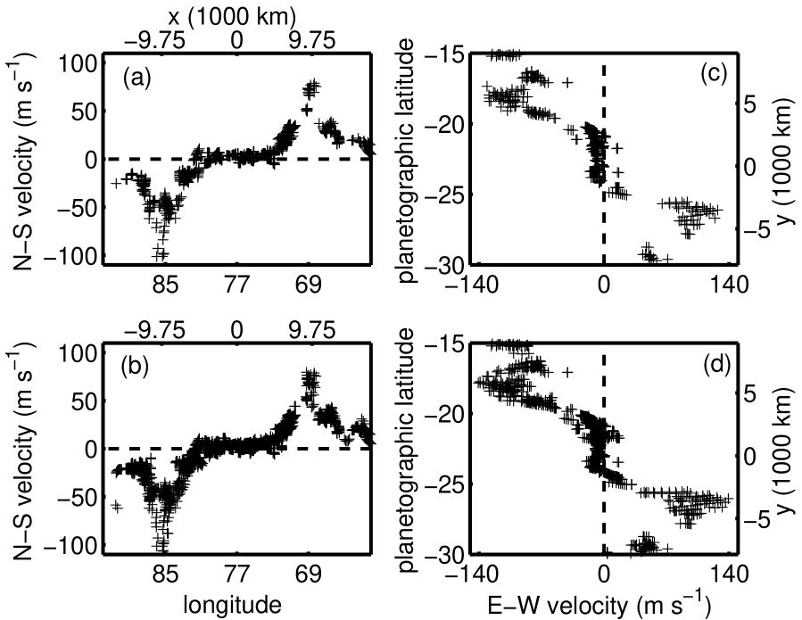
Figure 3: Parts (a) and (b) show the north-south component of the velocity from Fig. 1, for points that lie within $0.7^{\circ}$ and $1.4^{\circ}$ respectively, of the principal east-west axis. Parts (c) and (d) show the east-west component of the velocity for points that lie within $0.7^{\circ}$ and $1.4^{\circ}$ respectively, of the principal north-south axis. Parts (a), (b), (c), and (d) contain 903, 1992, 586, and 1163 points respectively.

3 Governing equations

3.1 1.5–layer reduced gravity QG approximation

We do not model the whole sphere, but only a domain that extends from $15^{\circ}$S to $30^{\circ}$S. For the flow in this domain, we adopt the 1.5–layer reduced gravity QG equations on a beta-plane (Ingersoll and Cuong, 1981). A derivation of the equations and the justification for their use can be found in Dowling (1995). Briefly, the layers correspond to an upper layer (also called “weather” layer) of constant density $\rho_{1}$ and a much deeper lower layer of constant density $\rho_{2}>\rho_{1}$. The upper layer contains the visible clouds and vortices while the lower layer contains a steady zonal flow. The two layers are dynamically equivalent to a single layer with rigid bottom topography $h_{b}$ and effective gravity $g\equiv g_{J}(\rho_{2}-\rho_{1})/\rho_{2}$, where $g_{J}$ is the true gravity in the weather layer, and the bottom topography is a parametrization of the flow in the lower layer. The governing equation for the system advectively conserves a potential vorticity $q$:

$$\frac{Dq}{Dt}\equiv\left(\frac{\partial}{\partial t}+\mbox{${\mathbf{v}}$}\cdot\nabla\right)q=0,$$ (1)

$$q(x,y,t)\equiv\nabla^{2}\psi-\frac{\psi}{L_{r}^{2}}+\frac{gh_{b}(y)}{L_{r}^{2}f_{0}}+\beta y.$$ (2)

Here $x$ and $y$ are the local E–W and N–S coordinates, $\psi$ is the streamfunction, $\mbox{${\mathbf{v}}$}\equiv{\bf\hat{z}}\times{\bf\nabla}\psi$ is the weather layer velocity, ${\bf\hat{z}}$ is the local vertical unit vector, $\beta$ is the local gradient of the Coriolis parameter $f(y)$, $f_{0}$ is the local value of $f(y)$, and $L_{r}$ is the local Rossby deformation radius. Since $g$ appears only in combination with $h_{b}$, we shall refer to $gh_{b}$ as the bottom topography. Restricting $gh_{b}$ to be a function of $y$ alone restricts the flow in the lower layer to be steady and zonal with no vortices. The case $gh_{b}=0$, or “flat” bottom topography, corresponds to the lower layer being at rest in the rotating frame.

3.2 The near-field

We assume that the GRS is a compact region (or patch) of anomalous potential vorticity. We denote the potential vorticity distribution of the GRS by $q^{GRS}(x,y)$, and for reasons that will become clear below, we refer to $q^{GRS}$ as the near-field. We define the streamfunction and velocity of the near-field to be:

$$q^{GRS}(x,y)\equiv\left(\nabla^{2}-1/L_{r}^{2}\right)\psi^{GRS}(x,y)$$ (3)

$$\mbox{${\mathbf{v}}$}^{GRS}\equiv{\bf\hat{z}}\times{\bf\nabla}\psi^{GRS}.$$ (4)

The velocity induced by a QG patch decays as exp($-r/L_{r}$), where $r$ is the distance from the patch boundary (Marcus, 1990, 1993). Due to the exponential decay of velocity, a region of fluid that contains the patch and whose average radius is a few $L_{r}$ greater than the patch radius will have a circulation (or integrated vorticity) that is approximately zero. It would therefore be incorrect under the QG approximation to refer to the vorticity of the GRS as anticyclonic since its net vorticity is zero. On the other hand, the potential vorticity of the GRS is anticyclonic, as is the vorticity of most of its quiescent interior and the inner portion of its high-speed collar, but the vorticity of the outer portion of its collar is cyclonic (which is easily verified by noting that the azimuthal velocity in that region falls off faster than $1/r$).

3.3 The far-field

The region of flow two or three deformation radii distant from the patch boundary, where the influence of the GRS is small, is defined to be the far-field. We assume the far-field flow to be zonal and independent of time and longitude. Eq. 2 then provides a relationship between the far-field velocity $\mbox{${\mathbf{v}^{\infty}}$}\equiv v_{x}^{\infty}(y){\bf\hat{x}}$, and the far-field potential vorticity $q^{\infty}(y)$:

$$q^{\infty}(y)=\left(\frac{d^{2}}{dy^{2}}-\frac{1}{L_{r}^{2}}\right)\psi^{\infty}(y)+\frac{gh_{b}(y)}{f_{0}L_{r}^{2}}+\beta y.$$ (5)

For all calculations in this paper, $v_{x}^{\infty}(y)$ is prescribed from Fig. 2 and the corresponding streamfunction $\psi^{\infty}$ from $-\int v^{\infty}_{x}\ dy$. At $22.5^{\circ}$S, which is the center of the domain, $\beta=4.6\times 10^{-12}$ m^-1 s^-1 and $f_{0}=-1.4\times 10^{-4}$ s^-1. Thus if $L_{r}$ were known, Eq. 5 shows that specifying $q^{\infty}$ is equivalent to specifying $gh_{b}$.

3.4 The interaction field

Let $q(x,y)$ be a steady solution of QG Eqs. 1–2 that consists of an anomalous patch of potential vorticity embedded in a far-field flow that is zonal and steady. We decompose $q$ into three components:

$$q(x,y)\equiv q^{\infty}(y)+q^{GRS}(x,y)+q^{INT}(x,y).$$ (6)

The superposition of $q^{GRS}$ and $q^{\infty}$ is not an exact solution because the far-field flow is deflected around the patch. We define the interaction potential vorticity $q^{INT}$ to represent the deflection of flow such that the total $q$ given by Eq. 6 is an exact solution of the QG equations. Note that by definition, $q^{INT}$ asymptotes to zero both far from and near the patch. We define the interaction streamfunction and velocity to be:

$$q^{INT}(x,y)\equiv\left(\nabla^{2}-1/L_{r}^{2}\right)\psi^{INT}(x,y)$$ (7)

$$\mbox{${\mathbf{v}}$}^{INT}\equiv{\bf\hat{z}}\times{\bf\nabla}\psi^{INT}.$$ (8)

With these definitions, the total velocity ${\mathbf{v}}$ and its streamfunction $\psi$ are superpositions of the near, interaction, and far-field components:

$$\psi=\psi^{\infty}+\psi^{GRS}+\psi^{INT}$$ (9)

$$\mbox{${\mathbf{v}}$}=\mbox{${\mathbf{v}}$}^{\infty}+\mbox{${\mathbf{v}}$}^{GRS}+\mbox{${\mathbf{v}}$}^{INT}.$$ (10)

Note that in the linear relationships between the potential vorticity and streamfunction given by Eqs. 5, 3, and 7, it is only the far-field component that contains the inhomogeneous bottom topography and $\beta$ terms.

4 Model definition

4.1 Model for far-field $q^{\infty}$

Laboratory experiments (Sommeria et al., 1989; Solomon et al., 1993) and numerical simulations (Cho and Polvani, 1996; Marcus et al., 2000) show that if the weather layer is stirred and allowed to come to equilibrium, the potential vorticity organizes itself into a system of east-west bands. The bands have approximately uniform $q$ and are separated by steep meridional gradients of $q$. The meridional gradients are all positive (i.e., have the sign as $\beta$) so that $q(y)$ monotonically increases from the south to the north pole like a “staircase”. The corresponding $\mbox{${\mathbf{v}}$}^{\infty}$ has alternating eastward-going and westward-going jet streams, with eastward-going jet streams occurring at every gradient or “jump”. Recent measurements (Read et al., 2006b) of the Jovian $q^{\infty}$ are not entirely consistent with this picture, for they show gradients near both eastward-going and westward-going jet streams. We therefore model $q^{\infty}$ between $30^{\circ}$S and $15^{\circ}$S by:

$$q^{\infty}(y)\equiv\sum_{i=1}^{2}\frac{\Delta Q_{i}}{2}\left(\tanh{\frac{y-y_{i}}{\delta_{i}}}+1\right).$$ (11)

The jumps for this model occur at $y_{i}$ and have strength $\Delta Q_{i}$, where $\Delta Q_{i}$ can be positive or negative. The strictly positive $\delta_{i}$ are a measure of the steepness of each jump. For all results in this paper, the jump locations were fixed at $y_{1}=26.0^{\circ}$S and $y_{2}=20.0^{\circ}$S, which are near the jet streams in Fig. 2. The free parameters for the model are $\Delta Q_{i}$ and $\delta_{i}$ for i=1,2. (Models with up-to four jumps near each jet stream were also tested, and the results were consistent with the ones presented here.)

4.2 Model for near-field $q^{GRS}$

We model the spatially compact $q^{GRS}$ as a piecewise-constant function obtained by the superposition of $M$ nested patches of uniform potential vorticity. The patches are labelled $i=1,2,\cdots,M$ from innermost to outermost patch. The principal E–W diameter of a patch is denoted by $(D_{x})_{i}$, and we define $q^{GRS}_{i}$ such that $q^{GRS}=q^{GRS}_{1}$ within the boundary of the innermost patch ($i=1$), $q^{GRS}=q^{GRS}_{2}$ between the boundary of the innermost patch ($i=1$) and the boundary of the next larger patch ($i=2$), and so on. The free parameters for the model are $M$, $q^{GRS}_{i}$, and $(D_{x})_{i}$ for $=1,2,\cdots,M$. Once the free parameters for $q^{GRS}$ and $q^{\infty}$ are specified, along with the value of $L_{r}$, the iterative method given in appendix B can be used to compute the interaction-field such that the total $q$ is a steady solution of the governing equations. Note that the shapes of patch boundaries are not free but are also computed by the iterative method.

5 Determination of best-fit parameter values

5.1 Decoupling of N–S velocity traits from far-field $q^{\infty}$

Here we show that the N–S velocity traits are insensitive to the far-field potential vorticity described by Eq. 11. Fig. 4 shows a model computed using the iterative method in appendix B for the parameter values given in Table 2. The middle column of Fig. 4 shows that for the E–W velocity along the N–S axis, all three velocity components, $\mbox{${\mathbf{v}}$}^{\infty}$, $\mbox{${\mathbf{v}}$}^{GRS}$, and $\mbox{${\mathbf{v}}$}^{INT}$, contribute significantly. However, the rightmost column shows that for the N–S velocity along the E–W axis, $\mbox{${\mathbf{v}}$}^{\infty}$ has no contribution (by definition), and the contribution of $\mbox{${\mathbf{v}}$}^{INT}$ is negligibly small. Only $\mbox{${\mathbf{v}}$}^{GRS}$ contributes significantly. We therefore conclude that the N–S traits depend primarily on parameters associated with $q^{GRS}$ and are insensitive to parameters associated with $q^{\infty}$. This decoupling leads to a logical order for determining the best-fit parameter values. The ordering is given in Table 1 and begins with the determination of $(D_{x})_{1}$ from the N–S traits. A more rigorous justification for the ordering is given in appendix C.

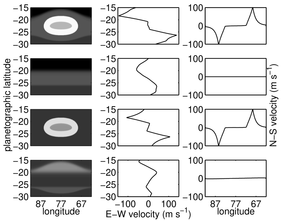
Figure 4: (left to right) Potential vorticity, E–W velocity along the N–S axis, and N–S velocity along the E–W axis. A gray-scale map is used for potential vorticity with black representing the most cyclonic fluid and white the most anticyclonic fluid. (top to bottom) The components due to the total $q$, the components due to $q^{\infty}$ alone, the components due to $q^{GRS}$ alone, and the components due to $q^{INT}$ alone. The total $q$ is a (uniformly translating) solution of the QG Equations. It was computed for the parameter values in Table 2 using the iterative method in appendix B. Note that the slivers of $q^{INT}$ (left column bottom row) are due to the displacement of the “jumps” or steep gradients in $q^{\infty}$ as they follow streamlines that deflect around the GRS.

Table 1: Relationship between an observable trait of the Great Red Spot and the model parameter that it determines. The ordering of the table, from top to bottom, is the order in which each model parameter is determined. A rigorous justification for the ordering is given in appendix C.

Observable trait	Model Parameter
Distance between peaks in N–S velocity along E–W axis	E–W diameter of GRS’s potential vorticity: $(D_{x})_{1}$
Magnitude of peak N–S velocity along E–W axis	Family of possible $q^{GRS}_{1}$ and $L_{r}$
N–S velocity along E–W axis for $|x|\geq(D_{x})_{1}/2$	Unique $q^{GRS}_{1}$ and $L_{r}$ from family
N–S velocity along E–W axis for $|x|\leq(D_{x})_{1}/2$	GRS’s interior potential vorticity: $q^{GRS}_{2}$, $(D_{x})_{2}$
E–W velocity along N–S axis	Far-field potential vorticity: $\Delta Q_{i}$, $\delta_{i}$

5.2 Determination of best-fit $L_{r}$ and $q^{GRS}$ from N–S velocity traits

Here we show that an $M=2$ model is sufficient to capture the N–S velocity traits to within the observational uncertainties. For brevity, the terms interior and exterior are used in reference to the regions $|x|<(D_{x})_{1}/2$ and $|x|>(D_{x})_{1}/2$ respectively.

For $M=1$, $q^{GRS}$ is a patch of uniform potential vorticity. Models were computed for different values of $(D_{x})_{1}$, $q^{GRS}_{1}$, and $L_{r}$. For each model, the peaks of the N–S velocity along the E–W axis were found to occur at $x=\pm(D_{x})_{1}/2$. The best-fit value of $(D_{x})_{1}=19500$ km was therefore inferred from trait 1 in $\S$2c. Next, the best-fit values of $q^{GRS}_{1}$ and $L_{r}$ were constrained using the observed peak magnitude $V^{NS}_{\rm max}$ of the N–S velocity along the E–W axis. In particular, for a given value of $L_{r}$, the value of $q^{GRS}_{1}$ was chosen so that the model reproduced the observed peak magnitude. By repeating this process for several values of $L_{r}$, a two–parameter family (i.e., a function of $L_{r}$ and $q^{GRS}_{1}$) of models that simultaneously capture the observed peak locations and peak magnitude was obtained. Some family members are shown in Fig 5. Note that the models do not capture the observed width of the northward and southward-going jets. In particular, for sufficiently small $L_{r}$ ($L_{r}=1300$ km), the model captures the rate of velocity fall-off in the interior but not in the exterior. For sufficiently large $L_{r}$ ($L_{r}=2400$ km) the opposite is true. For other values of $L_{r}$, the rate of fall-off is too fast or too slow in both regions. To overcome this shortcoming, models with $M=2$ were considered.

For $M=2$, $q^{GRS}$ is the superposition of two nested patches of uniform potential vorticity. Best-fit values of $L_{r}$, $q^{GRS}_{1}$, and $(D_{x})_{1}$ were taken from the $M=1$ model in Fig. 5 that captures the velocity profile in the exterior. As shown in Fig. 6, for $q^{GRS}_{2}=q^{GRS}_{1}$, the $M=2$ model does not capture the velocity profile in the interior. However, if $q^{GRS}_{2}$ is changed holding all other parameters fixed, only the interior flow changes (provided $(D_{x})_{1}-(D_{x})_{2}\geq 2L_{r}$). Thus with all other parameters fixed, a genetic algorithm (Zohdi, 2003) was used to determine values for $q^{GRS}_{2}$ and $(D_{x})_{2}$ that minimize the $L_{2}$-norm difference between the model N–S velocity along the E–W axis and the observed velocity in the interior. The parameter values obtained are listed in Table 2 and Fig. 7 shows that the N–S traits are captured for these parameter values. (Models with $M=3,4$ were also tested, and the results were consistent with the ones presented here.)

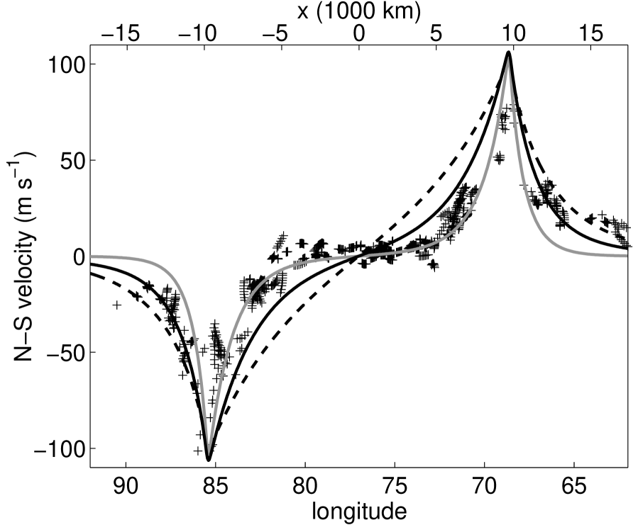
Figure 5: N–S velocity along the E–W axis for models with $M=1$. Crosses are Voyager 1 data from Fig. 3a. Solid black curve has $q^{GRS}_{1}=10.5\times 10^{-5}$ s^-1 and $L_{r}=2400$ km. Dashed curve has $q^{GRS}_{1}=6.5\times 10^{-5}$ s^-1 and $L_{r}=3800$ km. Solid gray curve has $q^{GRS}_{1}=19.5\times 10^{-5}$ s^-1 and $L_{r}=1300$ km. All models have the best-fit value of $(D_{x})_{1}=19500$ km and were computed using the iterative method in appendix B. The N–S velocity along the E–W axis is insensitive to parameters of the far-field because of decoupling as described in $\S$5a.

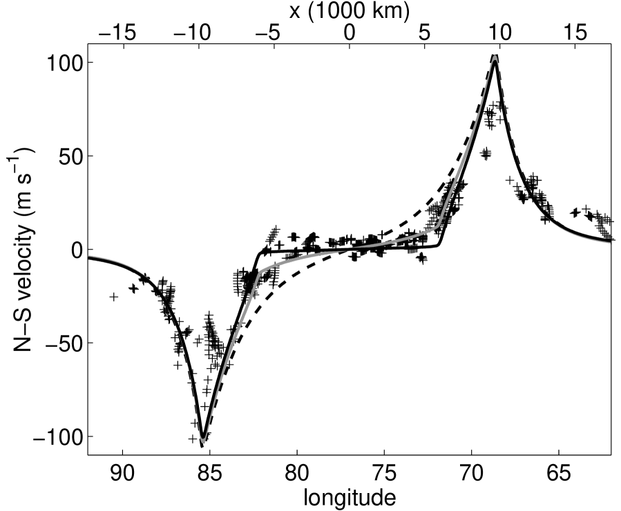
Figure 6: N–S velocity along the E–W axis for models with $M=2$. Each model has $L_{r}$, $(D_{x})_{1}$, $q^{GRS}_{1}$, and $(D_{x})_{2}$ set to the best-fit value in Table 2, but the values of $q^{GRS}_{2}$ for each model are different. The dashed curve has $q^{GRS}_{2}=q^{GRS}_{1}$, the solid gray curve has $q^{GRS}_{2}=0.8q^{GRS}_{1}$ and the solid black curve has the best-fit value of $q^{GRS}_{2}=0.57q^{GRS}_{1}$. Crosses are Voyager 1 data from Fig. 3a. The N–S velocity along the E–W axis is insensitive to parameters of the far-field because of decoupling as described in $\S$5a.

Table 2: Best-fit parameter values for $L_{r}$, $q^{GRS}$, and $q^{\infty}$.

Parameter	Best-fit value
$L_{r}$	2400 km
$M$	2
$q^{GRS}_{1}$	$10.5\times 10^{-5}$ s-1
$q^{GRS}_{2}$	$6.0\times 10^{-5}$ s-1
$(D_{x})_{1}$	19500 km
$(D_{x})_{2}$	12000 km
$\Delta Q_{1}$	$1.9\times 10^{-5}$ s-1
$\Delta Q_{2}$	$-5.6\times 10^{-5}$ s-1
$\delta_{1}$	300 km
$\delta_{2}$	1000 km

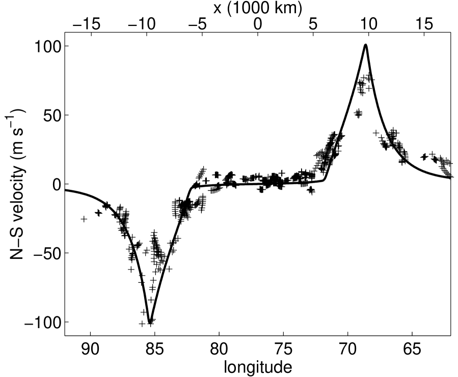
Figure 7: Solid line is the N–S velocity along the E–W axis for a model with best-fit parameter values given in Table 2. Crosses are Voyager 1 data from Fig. 3a.

5.3 Determination of best-fit $q^{\infty}$ from E–W velocity traits

The best-fit $q^{\infty}$ was determined from the E–W velocity traits. In particular, with the $q^{GRS}$ parameters fixed at their best-fit values from the preceding section, a genetic algorithm (Zohdi, 2003) was used to determine values for $\Delta Q_{i}$ and $\delta_{i}$ that minimize the $L_{2}$-norm difference between the model E–W velocity along the N–S axis and the corresponding observed velocity. The parameter values obtained are listed in Table 2. Fig. 8 shows that the E–W traits are captured for these parameter values. The corresponding $q^{\infty}$ is shown in Fig. 9. The velocities for this trait-capturing model were found to match the GRS velocities in Fig. 1 to within the observational uncertainties.

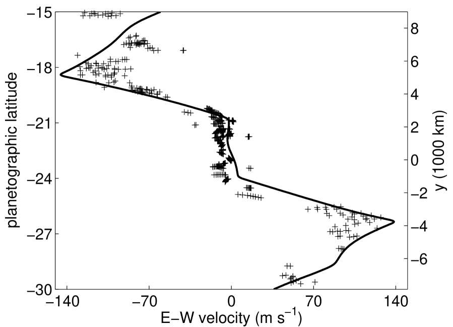
Figure 8: Solid line is the E–W velocity along the N–S axis for a model with best-fit parameter values given in Table 2. Crosses are Voyager 1 data from Fig. 3a.

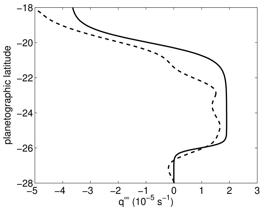
Figure 9: Solid line is far-field potential vorticity $q^{\infty}$ for model with best-fit parameters given in Table 2. Dashed line is $q^{\infty}$ determined in Dowling and Ingersoll (1989).

6 Physical implications of best-fit model

6.1 Cloud morphology and GRS’s potential vorticity anomaly

The models show that the peak north-south velocities along the principal east-west axis occur at $x=\pm(D_{x})_{1}/2$, where $(D_{x})_{1}$ is the principal east-west diameter of the GRS’s potential vorticity anomaly. Thus the best-fit value of $(D_{x})_{1}=19500$ km was inferred from trait 1 in $\S$2c. In fact, the models show that not just the east-west extremeties, but the entire boundary of the GRS’s potential vorticity anomaly is demarcated by the locations of peak velocity magnitude ($|{\bf v}|$). This implies that an estimate of the area and aspect ratio of the GRS’s potential vorticity anomaly can be made directly from the observed velocity field without first determining a best-fit model. Traditionally, the clouds associated with the GRS have been used to infer the area and aspect ratio of the vortex. The east-west diameter of the cloud cover associated with the GRS is $\approx$24000–26000 km in length, which is $\approx$25% longer than the east-west extent of the potential vorticity anomaly as determined by our best-fit model. The north-south diameter of the cloud cover is also $\approx$25% longer than that of the anomaly, so any estimate of the size of the GRS based on its cloud images rather than on its velocity overestimates the area of the potential vorticity anomaly by $\approx$50%.

6.2 Rossby deformation radius

The models show the rate of fall-off of the north-south velocity in the outer portion of the high-speed collar to be almost independent of all parameters with the exception of $L_{r}$. The models also show the magnitude of peak north-south velocity $V^{NS}_{\rm max}$ along the principal east-west axis to be approximately equal to the product of $L_{r}$, the potential vorticity $q^{GRS}_{1}$ in the collar, and a dimensionless number that depends weakly on $(D_{x})_{1}$/$L_{r}$ (see Table C1). Since $(D_{x})_{1}$ is known from the separation of the north-south peaks, and $V^{NS}_{\rm max}$ can be measured to within $\pm 7$ m s^-1, the best-fit values of $L_{r}=2400$ km and $q^{GRS}_{1}=10.5\times 10^{-5}$ s^-1 were determined simultaneously by demanding that the model reproduce the value of $V^{NS}_{\rm max}$ as well as the velocity fall-off in the outer portion of the collar.

6.3 Hollowness of GRS’s potential vorticity anomaly

The models show a uniform potential vorticity anomaly to be inconsistent with the north-south velocity along the east-west axis in the GRS’s high-speed collar. In particular, an anomaly with uniform potential vorticity cannot simultaneously capture the different rates at which the velocity falls-off in the inner and outer portion of the collar. However, a model with core potential vorticity $q^{GRS}_{2}\approx$60% of the collar’s potential vorticity $q^{GRS}_{1}$, is able to capture both fall-off rates to within the uncertainties. The “hollowness” of the GRS’s potential vorticity anomaly is surprising because other Jovian vortices such as the White Ovals, as well as other geophysical vortices such as the Antarctic Stratospheric Polar Vortex and Gulf Stream Rings, have uniform $|q|$ or a $|q|$ maximum in their cores. Furthermore, hollow vortices are sometimes unstable (Marcus, 1990). Initial-value simulations show that hollow vortices re-distribute their $q$ on an advective time scale so that the final $|q|$ is uniform or has a maximum in the core. This raises the question of how a hollow GRS is stabilized over time scales longer than an advective time scale.

6.4 Non-staircase far-field potential vorticity

The best-fit $q^{\infty}$ has a positive jump $\Delta Q_{1}$ of magnitude $1.9\times 10^{-5}$ s^-1 near the eastward-going jet stream and a larger, negative jump $\Delta Q_{2}$ of magnitude $5.6\times 10^{-5}$ s^-1 near the westward-going jet stream. Due to these opposing jumps, $q^{\infty}$ in this region does not monotonically increase with $y$. This is surprising because numerical and laboratory experiments (see $\S$4a) predict a monotonically increasing “staircase” profile, with jumps only at eastward-going jet streams. The best-fit profile determined here agrees qualitatively with a profile determined in Dowling and Ingersoll (1989) using an independent method.

6.5 Aspect ratio of GRS’s potential vorticity anomaly

The aspect ratio of the GRS’s potential vorticity anomaly is defined to be $(D_{x})_{1}/(D_{y})_{1}$, where $(D_{x})_{1}$ and $(D_{y})_{1}$ are the principal north-south and east-west diameters of the anomaly respectively. (Recall that the shape of the the GRS’s $q$ anomaly, and $(D_{y})_{1}$ in particular, are obtained as output from the iterative method in appendix B.) The aspect ratio of the anomaly depends on the ratio of $q^{GRS}_{1}$ to the shear of the ambient flow in which the GRS is embedded; a larger $q^{GRS}_{1}$ to ambient shear ratio implies a rounder vortex while a smaller ratio implies a more elongated vortex (Marcus, 1990). It should be emphasized that, in general, the ambient shear at the location of the GRS is not identical to the shear of the far-field flow $\mbox{${\mathbf{v}}$}^{\infty}$. Instead, as shown in Fig. 4, the ambient shear is determined by the interaction of the GRS with the far-field flow. In particular, the middle column of Fig. 4 shows that $\mbox{${\mathbf{v}}$}^{INT}$ is large and produces a shear with half the magnitude and opposite sign to the shear of $\mbox{${\mathbf{v}}$}^{\infty}$. Therefore, the effect of $\mbox{${\mathbf{v}}$}^{INT}$ is to greatly reduce the ambient shear at the location of the GRS. For the best-fit model, the aspect ratio of the anomaly is 2.18. If the mitigating effect of $\mbox{${\mathbf{v}}$}^{INT}$ on the shear is eliminated by setting $\Delta Q_{i}=0$, with all other parameters, in particular $(D_{x})_{1}$, unchanged from their best-fit values, then the GRS’s anomaly shrinks in the north-south direction (i.e., $(D_{y})_{1}$ decreases) so that its aspect ratio is increased by $\approx$28%.

The panel in the left column and bottom row of Fig. 4 explains the functional dependence of $\mbox{${\mathbf{v}}$}^{INT}$ on $y$ and why its shear is adverse to the local shear of $\mbox{${\mathbf{v}}$}^{\infty}$. The panel shows that the effect of deflecting the jet streams and associated isocontours of $q^{\infty}$ around the GRS is equivalent to placing nearly semi-circular patches of $q$ north and south of the GRS. When the isocontours of $q^{\infty}$ that are deflected south of the GRS have latitudinal gradient $dq^{\infty}/dy>0$, the semi-circular patch of $q$ south of the GRS produces anticyclonic shear at the latitude of the GRS. Similarly, if the isocontours that are deflected north of the GRS have $dq^{\infty}/dy>0$, the semi-circular patch of $q$ north of the GRS produces cyclonic shear at the latitude of the GRS. Thus if the eastward-going and westward-going jet streams of $\mbox{${\mathbf{v}}$}^{\infty}$, which are deflected respectively south and north of the GRS, both had $dq^{\infty}/dy>0$, then the two semi-circular patches of vorticity in Fig. 4 would have opposite sign and form a dipole. The dipole would create a large net westward flow at the latitude of the GRS, but would create little shear (none, if the patches had equal strength) there. However, for the best-fit model, the westward-going jet stream has $dq^{\infty}/dy<0$ and the eastward-going jet stream has $dq^{\infty}/dy>0$. Both semi-circular patches are anticyclonic and the result is a large shear that is adverse to the shear of $\mbox{${\mathbf{v}}$}^{\infty}$, as shown in Fig. 4.

7 Conclusions and Future Work

In this paper we have described a technique for determining quantities of dynamical significance from the observed velocity fields of a long-lived Jovian vortex and its neighboring jet streams. Our approach was to model the flow using the simplest governing equation and the fewest unknown parameters that would reproduce the observed velocity to within its observational uncertainties. For the Voyager 1 data, this is a nine-parameter model that is an exact steady solution to the 1.5–layer reduced gravity QG equations. The nine parameters are the local Rossby deformation radius, the $q$ in the GRS’s high-speed collar, the $q$ in the GRS’s core, the east-west diameter of the GRS’s $q$ anomaly, the east-west diameter of the GRS’s core, the size and steepness of two jumps in the far-field $q$, one located near the latitude of the eastward-going jet stream to the south of the GRS, and the other located near the westward-going jet-stream to its north. We determined “best-fit” values for the nine parameters by identifying several “traits” of the observed GRS velocity field and seeking a model that reproduced all those traits.

Perhaps the most surprising result of our study was that the simple model described above was able to reproduce the entire observed velocity field in Fig. 1 to within the uncertainties of 7% (that is, 7 m s^-1). The success of the model is due, in part, to the fact that the GRS must be well-described by the QG equations, and to the fact that the model is an exact steady solution of the governing equations. The success is also due to the fact that the chosen traits are robust and in some sense unique (e.g., hollowness) to the physics associated with the GRS. Finally, a part of the success of the model is due to the relatively large uncertainties (7%) of the Voyager 1 velocities compared to more recent data sets (see below).

Our most important result was to show that the interaction between the GRS and its neighboring jet streams determines the shape of the GRS’s $q$ anomaly. By explicitly computing the interaction, we showed that the effect of the GRS is to bend the jet steams (identified by their jumps in $q$) so that they pass around the GRS, and the effect of the bending of the jet streams is to reduce the zonal shear at the location of the GRS. A smaller zonal shear at the location of the GRS compared to the $q$ of the GRS implies a smaller east-west to north-south aspect ratio for the GRS’s $q$ anomaly. The best-fit model has a positive jump at the eastward-going jet stream and a larger, negative jump at the westward-going jet stream. The bending of these opposing jumps significantly reduces the zonal shear at the GRS, making the aspect ratio of the GRS’s $q$ anomaly $\approx$28% smaller (i.e., rounder) than it would be if there were no interaction with the jet streams. It is also interesting to note that due to the opposing jumps, the far-field $q$ does not monotonically increase from south to north, which is contrary to numerical and laboratory experiments that predict a monotonically increasing “staircase” profile.

The GRS’s potential vorticity anomaly was found to be “hollow” with core potential vorticity $\approx$60% that of the collar; this is curious because hollow vortices are generally unstable. The locations of peak velocity magnitude were found to be accurate markers of the boundary of the GRS’s $q$ anomaly, which implies that the area and aspect ratio of the anomaly can be inferred directly from the velocity data. On the other hand, clouds associated with the GRS are not an accurate marker of the anomaly as they differ from the anomaly area by $\approx$50%. This suggests that cloud aspect ratios, areas, and morphologies should not be used to determine temporal variability of Jovian vortices.

In devising the model, our philosophy was to include no more complexity than was required to match the observed velocity to within its uncertainties. However, lower-uncertainty measurements of the velocity field using CIV (Asay-Davis et al., 2006) on observations from Hubble Space Telescope, Cassini, and Galileo, may require that the QG approximation be relaxed in favor of shallow-water. Also, if thermal observations (Read et al., 2006a) are to be accounted for, governing equations that permit 3D baroclinic effects will be required. Modeling different data sets would show how the best-fit parameter values evolve with time.

A companion paper to this one shows that the best-fit model is stable and explores the stabilizing effects of the hollow GRS–jet stream interaction. Demonstrating stability is important because hollow vortices are usually unstable. Finally, there are several questions raised by our best-fit model of the GRS that will need to be answered. How did a hollow GRS form? Why are there no other hollow Jovian vortices (for which the velocity has been measured, cf. the current Red Oval and the three White Ovals at 33^∘S, which existed between the mid-1930’s and 1998)? One possible answer to the second question is that Jovian vortices apart from the GRS lack opposing jumps near their neighboring jet streams and the associated reduction in shear due to the vortex–jet stream interaction. Indeed, a preliminary best-fit model of the White Ovals (Shetty et al., 2006) does not show opposing jumps near the neighboring jet streams.

Appendix A Method for removing spurious velocities and correcting for the curvature of cloud trajectories

The method involves two stages of iteration. We start with the velocity from Mitchell et al. (1981) in which the trajectories are assumed to be straight lines and the velocities are assumed to be located mid-way between tie-point pairs (the initial and final coordinates of a cloud feature in a pair of images is defined to be a tie-point pair). We then spline the irregularly spaced tie-point velocities onto a uniform grid of size $0.05^{\circ}\times 0.05^{\circ}$. The first step of the inner loop of the iteration computes, for each tie-point pair, the curved trajectory that a passive Lagrangian particle would follow beginning at the initial tie-point location ($x_{I},y_{I}$) to its final tie-point location ($x_{F},y_{F}$), using a $5^{th}$-order Runge-Kutta integration. To carry out the integration, the velocity field is spline-interpolated from the grid to the off-grid locations where it is required by the integrating scheme. The integration creates a set of closely spaced points, $(x_{i},y_{i})$, $i=1,2,3,\cdots,N$, along the trajectory, where $(x_{1},y_{1})\equiv(x_{I},y_{I})$. In general, this trajectory does not end with $(x_{N},y_{N})$ equal to $(x_{F},y_{F})$ as desired. We therefore compute a second trajectory $(X_{i},Y_{i})$ starting from the final tie–point location $(x_{F},y_{F})$ and integrate backward in time using the interpolated velocity from grid points. A third trajectory $(\bar{x}_{i},\bar{y}_{i})\equiv[(N-i)(x_{i},y_{i})+(i-1)(X_{i},Y_{i})]/(N-1)$ is then computed as a linear interpolation that, by construction, starts at $(x_{I},y_{I})$ and ends at $(x_{F},y_{F})$. Moreover, because the points along each trajectory are close together, the velocity at each point $(\bar{x}_{i},\bar{y}_{i})$ is well-approximated with the temporal, second-order finite difference derivative using the nearest neighbor trajectory points. A new velocity at the grid points is created from the spline of the velocities along the curved trajectories of all of the tie-point pairs (for each trajectory, we use the velocities at eight approximately equally spaced points along the trajectory). We then return to the first step of the inner loop. We use the original set of tie-point pairs, but the velocity is now the updated velocity on the grid. The inner loop is iterated until it converges (typically, three iterations). We then compute the residual of each velocity vector, which is defined to be the magnitude of the difference between the original, uncorrected tie-point velocity and the converged velocity interpolated by splines to that location. Velocity vectors with residuals that were six times the root-mean-squared value of all of the residuals were considered to be spurious, and their tie-points were removed from the original data set. Once the spurious points are removed, the outer loop is complete and the entire process is repeated starting with the new (diminished) set of tie-points. The outer loop was iterated until no more tie points were removed. The Voyager 1 tie-point set required three iterations of the outer loop and resulted in the removal of 220 of the original 1100 points. The root-mean-squared residual of the iterated velocity is $\approx 7$ m s^-1, and we use this value as a measure of the uncertainty in the data. For comparison, it should be noted that the residual of the Voyager 1 tie-points without correcting for curvature and without removing spurious tie-points is $\approx 9$ m s^-1, and the residual for the Hubble Space Telescope data (from CIV) for the GRS using the method described here is $\approx 3$ m s^-1 (Asay-Davis et al., 2006). In the high-speed collar, the residuals in the vorticity derived by differentiating the Voyager 1 velocity are $\approx 35\%$ of the maximum vorticity.

Appendix B Iterative method for computing steady-state solutions of the 1.5–layer reduced gravity QG equations

Here we describe an iterative method for computing steady solutions of Eqs. 1–2 subject to periodic boundary conditions in $x$ and $y$. The method seeks solutions that consist of a single anomalous patch embedded in a zonal flow, and that are steady when viewed in a frame translating with the patch. Such solutions are of the form $q(x,y,t)=q(x-Ut,y)$, where $U\bf{\hat{x}}$ is the constant drift velocity of the vortex. Substituting for $q$ in Eq. 1 we obtain:

$$({\mbox{${\mathbf{v}}$}}-U{\bf\hat{x}})\cdot{\mbox{${\mathbf{\nabla}}$}}q=0,$$ (12)

which implies that isocontours of $q$ and isocontours of $\psi+Uy$ are coincident. It is this property that the iterative method exploits to compute uniformly translating solutions. As input, the method requires $L_{r}$, $q^{GRS}_{i}$, $(D_{x})_{i}$ for $i=1,2,\cdots,M$, and $\Delta Q_{i}$, $\delta_{i}$ for $i=1,2$. As output, the method provides $q^{INT}$, $U$, and the shape of each vortex patch. Initial guesses must be supplied for the quantities obtained as output. The guesses are then iterated, keeping the input quantities fixed, until the total $q$ is a uniformly translating solution. The iterative procedure is described below. The domain is $x\in[-L_{x},L_{x}]$, $y\in[-L_{y},L_{y}]$. The origin is at the point of intersection of the principal axes.

• A new $\psi$ is computed from the current $q$ by inverting the Helmholtz operator in Eq. 2. The current $q$ is the sum of $q^{\infty}$, the current $q^{GRS}$, and the current $q^{INT}$.

• A new drift speed $U$ for the anomaly is computed. The drift speed of the anomaly, as derived in Marcus (1993), is given by $\int_{A}q^{GRS}v_{x}dA/\int_{A}q^{GRS}dA$, where $A$ is the current area of the anomaly.

• New isocontours of $(\psi+Uy)$ are computed. The isocontours are streamlines of the current velocity in the translating frame. Streamlines that extend from the western to the eastern boundary of the domain are referred to as open streamlines. Streamlines that are not open are referred to as closed.

• A new $q^{INT}$ is computed. This is done by setting the value of $q$ along an open streamline to the value of $q^{\infty}$ at the point on the western boundary through which the streamline passes. In other words, if $y=s(x)$ is the equation of an open streamline, then $q(x,s(x))\equiv q^{\infty}(s(-L_{x}))$ for $x\in[-L_{x},L_{x}]$.

• A new $q^{GRS}$ is computed by computing a new boundary for patches $i=1,2,\cdots,M$. The new boundary is identified as the closed streamline that passes through $x=(D_{x})_{i}/2$. Note that if the current patch is reflection symmetric about the N–S axis, the value of $(D_{x})_{i}$ is conserved. The potential vorticity of each patch $q^{GRS}_{i}$ is held fixed.

The iterations are repeated until $U$ converges to within a desired tolerance, or equivalently, until isocontours of $(\psi+Uy)$ and isocontours of $q$ are coincident. For all calculations in this paper, the initial guess for the shape of a patch was an ellipse with $(D_{y})_{i}=0.5(D_{x})_{i}$. The final shapes are reflection symmetric about the N–S axis, but they are not symmetric about the E–W axis. The initial $q^{INT}$ and $U$ were set to zero. The grid resolution was $0.05^{\circ}\times 0.05^{\circ}$. The equilibria are not sensitive to the domain size provided the domain boundaries are at least three deformation radii away from the edge of the outermost patch. We note that it would be interesting to explore initial guesses that are not reflection symmetric about the N–S axis, to see if asymmetry persists for the final solution. Indeed, recent low-uncertainty measurements of the GRS velocity field (Asay-Davis et al., 2006) show asymmetry about the N–S axis. For the Voyager 1 data set however, any asymmetry is much smaller than the uncertainties, so asymmetric models are deferred to future work.

Appendix C Sensitivity of model traits to model parameters

Here we quantify the sensitivity of a model trait to small changes in a model parameter. The results justify the methodology used in $\S$5 to determine the best-fit parameter values. Consider a trait of the N–S velocity along the E–W axis, say the peak magnitude $V^{NS}_{\rm max}$. From dimensional analysis it is rigorous to write:

$$V^{NS}_{\rm max}=L_{r}q^{GRS}_{1}\,F[q^{GRS}_{2}/q^{GRS}_{1},\Delta Q_{1}/q^{GRS}_{1},\Delta Q_{2}/q^{GRS}_{1},\delta_{1}/L_{r},\delta_{2}/L_{r},(D_{x})_{1}/L_{r},(D_{x})_{2}/L_{r}],$$ (13)

where $F$ is a dimensionless function of seven dimensionless arguments (note that Eq. 13 is completely general if the value of $V^{NS}_{\rm max}$ is independent of $\mbox{${\mathbf{v}}$}^{\infty}$ as is suggested by decoupling; otherwise, and in particular, for any trait of the E–W velocity along the N–S axis, the function $F$ would have to include arguments of the dimensionless scalars that parametrize $\mbox{${\mathbf{v}}$}^{\infty}$). The sensitivity of $V^{NS}_{\rm max}$ to changes in a particular parameter, say $L_{r}$, was determined by computing the value of $V^{NS}_{\rm max}$ for a change in $L_{r}$ of $\pm$5% around its best-fit value with all other parameters fixed at their best-fit values, and then using a finite difference scheme to construct the dimensionless partial derivative $(L_{r}/V^{NS}_{\rm max})\,(\partial V^{NS}_{\rm max}/\partial L_{r})$ $\equiv$ $\partial\,ln\,V^{NS}_{\rm max}/\partial\,ln\,L_{r}$. Dimensionless partial derivatives computed for other traits are listed in Table 3. We consider a trait to be insensitive to any parameter for which the absolute value of its dimensionless partial derivative is much less than unity. Note that the results are consistent with Table 1.

The partial derivatives are not independent. For example, four of the parameters in Eq. 13 have dimensions of inverse time (and we write them as $\tau_{i}$, $i=1,2,3,4$), and four have dimensions of length (and we write them as $\chi_{i}$, $i=1,2,3,4$). Differentiation of Eq. 13 yields the following constraints:

$$\sum_{i=1}^{4}\partial\,ln\,V^{NS}_{\rm max}/\partial ln\,\tau_{i}\equiv 1,$$ (14)

and

$$\sum_{i=1}^{4}\partial\,ln\,V^{NS}_{\rm max}/\partial ln\,\chi_{i}\equiv 1.$$ (15)

In general, a trait $L$ that has dimensions of length, such as the width of the N–S jet, and which depends only on the parameters in Eq. 13, must satisfy the following constraints:

$$\sum_{i=1}^{4}\partial\,ln\,L/\partial\,ln\,\tau_{i}\equiv 0,$$ (16)

and

$$\sum_{i=1}^{4}\partial\,ln\,L/\partial\,ln\,\chi_{i}\equiv 1.$$ (17)

Table 3 shows that all traits with the exception of $(D_{y})_{1}$ satisfy the constraints. The reason $(D_{y})_{1}$ does not satisfy the constraints is that it is a trait of the E–W velocity and therefore also depends on parameters associated with the far-field flow $\mbox{${\mathbf{v}}$}^{\infty}$.

The uncertainties in the best-fit parameter values may be quantified as follows. The $L_{2}$ norm difference between the best-fit velocity and the velocity in Fig. 1 is computed. The $L_{2}$ norm difference is then recomputed with all parameters fixed at their best-fit values with the exception of parameter $L_{r}$ (say). A curve of the $L_{2}$ norm difference as a function of $L_{r}$ is then computed. By construction, the curve has a minimum at the best-fit value of $L_{r}$. The width of the curve at half-minimum is identified as the uncertainty in $L_{r}$. Since measurements of the GRS velocity using CIV have much lower uncertainties than the Voyager velocity and will soon be available (Asay-Davis et al., 2006), we did not deem it useful to compute parameter uncertainties for the analyses in this paper.

Table 3: Sensitivity of model traits to model parameters. Each entry is (parameter/trait) $\,\times\,$ $\partial$(trait)/$\partial$(parameter) $\equiv$ $\partial\,ln\,$(trait)/$\partial\,ln\,$(parameter). The partial derivatives were evaluated at the best-fit parameter values in Table 2. The full-width-at-half-maximum ($W$) for the northward-going jet along the principal east-west axis is broken into two pieces $W\equiv E+I$. $E$ (or $I$) is the distance along the east-west axis between the location where the north-south velocity reaches its maximum value of $V^{NS}_{\rm max}$, and the location in the outer (or inner) portion of the high-speed collar where the north-south velocity falls to $V^{NS}_{\rm max}/2$. Since the models are reflection symmetric about the principal north-south axis (due to the reflection symmetric initial guess, see appendix B), the northward-going and southward-going jets have identical values of $V^{NS}_{\rm max}$, $I$, and $E$.

Model trait $\downarrow$ / Model parameter $\rightarrow$	$(D_{x})_{1}$	$L_{r}$	$q^{GRS}_{1}$	$q^{GRS}_{2}$	$(D_{x})_{2}$	$\Delta Q_{1}$	$\Delta Q_{2}$	$\delta_{1}$	$\delta_{2}$
Peak N–S velocity along E–W axis, $V^{NS}_{\rm max}$	0.3	1.0	1.1	0.0	-0.2	0.1	-0.1	0.0	0.0
Distance between N–S peaks along E–W axis	1.0	0.0	0.0	0.0	0.0	0.0	0.0	0.0	0.0
Exterior width of N–S jets at half maximum, $E$	0.1	1.0	0.1	0.0	-0.1	0.0	0.0	0.0	0.0
Interior width of N–S jets at half maximum, $I$	1.1	0.5	0.0	-0.1	-0.7	0.1	-0.1	0.0	0.1
N–S diameter of GRS’s potential vorticity, $(D_{y})_{1}$	0.6	1.1	0.4	-0.1	-0.3	0.1	-0.3	0.0	0.0

References

- Asay-Davis et al. (2006) Asay-Davis, X., S. Shetty, and P. Marcus, 2006: Extraction of Velocity Fields from Telescope Image Pairs of Jupiter’s Great Red Spot, New Red Oval, and Zonal Jet Streams. Bulletin of the American Physical Society, 51, 116.
- Cho and Polvani (1996) Cho, J.-K. and L. Polvani, 1996: The emergence of jets and vortices in freely evolving, shallow water turbulence on a sphere. Physics of Fluids, 8, 1531–1552.
- Cho et al. (2001) Cho, J. Y.-K., M. de la Torre Juarez, A. P. Ingersoll, and D. G. Dritschel, 2001: High-resolution, three-dimensional model of jupiter’s great red spot. J. Geophys. Res., 106, 5099–5106.
- Dowling (1995) Dowling, T. E., 1995: Dynamics of jovian atmospheres. Annual Review of Fluid Mechanics, 27, 293–334.
- Dowling and Ingersoll (1988) Dowling, T. E. and A. P. Ingersoll, 1988: Potential vorticity and layer thickness variations in the flow around jupiter’s great red spot and the white oval bc. J. Atmos. Sci., 45, 1380–1396.
- Dowling and Ingersoll (1989) — 1989: Jupiter’s great red spot as a shallow water system. J. Atmos. Sci., 46, 3256–3278.
- Ingersoll and Cuong (1981) Ingersoll, A. P. and P. G. Cuong, 1981: Numerical model of long-lived jovian vortices. J. Atmos. Sci., 38, 2067–2076.
- Limaye (1986) Limaye, S. S., 1986: Jupiter: New estimates of the mean zonal flow at the cloud level. Icarus, 65, 335–352.
- Marcus (1990) Marcus, P. S., 1990: Vortex dynamics in a shearing zonal flow. J. Fluid Mech., 215, 393–430.
- Marcus (1993) — 1993: Jupiter’s great red spot and other vortices. Rev. Astron. Astrophy., 31, 523–573.
- Marcus et al. (2000) Marcus, P. S., T. Kundu, and C. Lee, 2000: Vortex dynamics and zonal flows. Physics of Plasmas, 7, 1630–1640.
- Mitchell et al. (1981) Mitchell, J. L., R. F. Beebe, A. P. Ingersoll, and G. W. Garneau, 1981: Flow fields within jupiter’s great red spot and white oval bc. J. Geophys. Res., 86, 8751–8757.
- Read et al. (2006a) Read, P. L., P. J. Gierasch, and B. J. Conrath, 2006a: Mapping potential-vorticity dynamics on Jupiter. II: the Great Red Spot from Voyager 1 and 2 data. Quarterly Journal of the Royal Meteorological Society, 132, 1605–1625.
- Read et al. (2006b) Read, P. L., P. J. Gierasch, B. J. Conrath, A. Simon-Miller, T. Fouchet, and Y. Y. H, 2006b: Mapping potential-vorticity dynamics on Jupiter. I: Zonal-mean circulation from Cassini and Voyager 1 data. Quarterly Journal of the Royal Meteorological Society, 132, 1577–1603.
- Shetty et al. (2006) Shetty, S., X. Asay-Davis, and P. S. Marcus, 2006: Modeling and Data Assimilation of the Velocity of Jupiter’s Great Red Spot and Red Oval. Bulletin of the American Physical Society, 51, 116.
- Simon-Miller et al. (2002) Simon-Miller, A. A., P. J. Gierasch, R. F. Beebe, B. Conrath, F. M. Flasar, R. K. Achterberg, and the Cassini CIRS Team, 2002: New observational results concerning jupiter’s great red spot. Icarus, 158, 249–266.
- Solomon et al. (1993) Solomon, T., W. Holloway, and H. Swinney, 1993: Shear flow instabilities and rossby waves in barotropic flow in a rotating annulus. Physics of Fluids, 5, 1971–1982.
- Sommeria et al. (1989) Sommeria, J., S. D. Meyers, and H. L. Swinney, 1989: Laboratory model of a planetary eastward jet. Nature, 337, 58–61.
- Zohdi (2003) Zohdi, T. I., 2003: Genetic design of solids possessing a random-particulate microstructure. Philosophical Transactions of the Royal Society A: Mathematical, Physical and Engineering Sciences, 361, 1021–1043.