Spontaneous emission from a two–level atom tunneling in a double–well potential

Abstract

We study a two-level atom in a double–well potential coupled to a continuum of electromagnetic modes (black body radiation in three dimensions at zero absolute temperature). Internal and external degrees of the atom couple due to recoil during emission of a photon. We provide a full analysis of the problem in the long wavelengths limit up to the border of the Lamb-Dicke regime, including a study of the internal dynamics of the atom (spontaneous emission), the tunneling motion, and the electric field of the emitted photon. The tunneling process itself may or may not decohere depending on the wavelength corresponding to the internal transition compared to the distance between the two wells of the external potential, as well as on the spontaneous emission rate compared to the tunneling frequency. Interference fringes appear in the emitted light from a tunneling atom, or an atom in a stationary coherent superposition of its center–of–mass motion, if the wavelength is comparable to the well separation, but only if the external state of the atom is post-selected.

I Introduction

Young’s double slit experiment, in which interference is observed from light passing through two small slits or holes in a plate placed at a distance comparable to the wavelength of the light, constitutes one of the experiments at the base of quantum mechanics. Theory and experiment have been refined over the years to the point that the two holes have been replaced by two trapped atoms or ions which scatter incoming laser light Lenz and Meystre (1993); Eichmann et al. (1993); Itano et al. (1998); Agarwal et al. (2002); Feagin (2006); Wickles and Müller (2006). With the advance of the coherent control of the external degrees of freedom of atoms (see e.g. Sebby-Strabley et al. (2006); Shin et al. (2004); Hänsel et al. (2001); Treutlein et al. (2006)), the realization of atom interferometers Carnal and Mlynek (1991); Keith et al. (1991); Hackermüller et al. (2004) (see Miffre et al. (2006) for a recent review), and in particular the realization of Schrödinger cat states of the center–of–mass coordinate of a single atom or ion Monroe et al. (1996), it is natural to ask if interference could be observed in the light emitted from a single atom superposed coherently in two different positions. A similar question was answered to the negative in a paper by Cohen-Tannoudji et al. Cohen-Tannoudji et al. (1992) for the case of scattering of light from a massive object brought into orthogonal position states. The physical reason is clear: interference can only arise if the probe particle can distinguish the two locations of the target. But then the probe particle must get entangled with the target. If the target is massive its two orthogonal position states remain unaltered during scattering, and therefore lead to vanishing overlap of the scattered probe states after tracing out the target. Later the scattering problem was reconsidered for lighter targets, where it was shown that interference can arise. In particular, Rohrlich et al. Rohrlich et al. (2006) analyzed the general situation of the scattering of two free particles, a probe with mass $m$ and a target with mass $M$. Interference was predicted for the case of $m\simeq M$, and even perfect visibility of interference fringes for $m=M$ in one dimension.

Similarly, Schomerus and coworkers Schomerus et al. (2002) analyzed the scattering of particles from a “quantum obstacle”, an obstacle brought into a coherent superposition of positions. An important difference to Rohrlich et al. (2006) lies in the fact that the target was supposed to be bound in a double–well potential and to tunnel coherently between the two wells with tunneling frequency $\Delta$. For the case of one dimensional scattering, they showed that the quantum obstacle leads to almost the same transmission resonances as two fixed obstacles, if the kinetic energy $\epsilon$ of the incident particle satisfies $\epsilon\ll\Delta$. In the opposite limit, interference can still be recovered by post-selecting the elastic scattering channel.

Spontaneous emission is not the same as scattering, and it is a priori unclear if these results apply to spontaneous emission alone as well. Furthermore, the properties of the emitted light are only a small part of the interesting physics that can arise, if internal and external degrees of the tunneling atom are coupled. Indeed, one might ask, if spontaneous emission itself (e.g. the decay rates of the excited level) changes, if the atom is brought into a coherent superposition of different external states. Also, what happens with the tunneling motion? To what extent does the emitted photon cause decoherence of the external degree of freedom? Spontaneous emission from a tunneling two–level atom was considered in Japha and Kurizki (1996) for the case of the transmission of an atom through a rectangular energy barrier in one dimension with the atom coupled to a one dimensional mode continuum. It was shown that the recoil from photon emission can lift the atom over the tunnel barrier and thus increase significantly the transmission.

In the present paper we examine spontaneous emission of a two–level atom trapped in a double–well potential, where the atom interacts with the full three dimensional continuum of electromagnetic modes (the interaction with a single cavity mode was treated in Martin and Braun ). We carefully investigate the effective dynamics of all three subsystems involved: the internal degree of freedom of the atom, the tunneling motion, and the electric field created by the emitted photon in a regime where the photon wavelength is at most comparable to the well separation. The tunneling motion may suffer decoherence from the emission of a photon from the atom, but this depends, amongst other things, on the timing of the emission of the photon. Interference in the light emitted from the atom is very weak, but interference with perfect visibility of the fringes arises if the external state of the atom is post-selected in the energy basis.

II Model

II.1 Derivation of the Hamiltonian

We consider a trapped two-level atom (with levels $|g\rangle$, $|e\rangle$ of energy $\mp\hbar\omega_{0}/2$ respectively) interacting with traveling modes of the electromagnetic field as illustrated in Fig. 1. The atom is assumed to be tightly bound in the $x-y$ plane at the equilibrium position $x=y=0$ and to experience a symmetric double–well potential $V(z)$ along the $z$ direction.

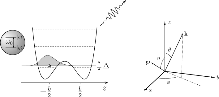
Figure 1: Two-level atom in a double–well potential interacting with a continuum of electromagnetic waves. Right panel: coordinate system used, with the atom tunneling in $z$-direction, and the atomic dipole in the $x-z$-plane

The Hamiltonian of this system is given by

$$H=H_{A}+H_{F}+H_{AF},$$ (1)

where $H_{A}=H_{A}^{\mathrm{ex}}+H_{A}^{\mathrm{in}}$ denotes the Hamiltonian of the trapped atom, $H_{F}$ is the Hamiltonian of the free field and $H_{AF}$ is the interaction Hamiltonian describing the atom–field interaction. Explicitly,

$$H_{A}^{\mathrm{ex}}=\frac{p_{z}^{2}}{2M}+V(z),$$ (2)

$$H_{A}^{\mathrm{in}}=\frac{\hbar\omega_{0}}{2}\sigma_{z}^{\mathrm{in}},$$ (3)

$$H_{F}=\hbar\sum_{k}\omega_{k}a_{k}^{\dagger}a_{k},$$ (4)

and, in dipole approximation,

$$H_{AF}=-\sum_{k}\mathbf{d.E}_{k}$$ (5)

where $\mathbf{d}$ is the atomic dipole operator and

$$\mathbf{E}_{k}={\cal E}_{k}\mbox{\boldmath{$\epsilon$}}_{k}\left(a_{k}e^{i{\bf k}.{\bf R}}+a_{k}^{\dagger}e^{-i{\bf k}.{\bf R}}\right)$$ (6)

the electric field operator, ${\cal E}_{k}=\sqrt{\frac{\hbar\omega_{k}}{2\epsilon_{0}V}}$, $\epsilon_{0}$ is the permittivity of free space, $V$ the electromagnetic mode quantization volume, $\mbox{\boldmath{$\epsilon$}}_{k}$ the electric field polarization vector (normalized to length one), $k$ stands for wave number ${\bf k}=(k_{x},k_{y},k_{z})$ and polarization $\lambda=1,2$ of the electromagnetic modes with frequency $\omega_{k}=c|{\bf k}|$ (where $c$ is the speed of light in vacuum), and ${\bf R}=(x,y,z)$ for the center–of–mass position of the atom. Note that in Eqs. (2)–(6) $z$ is still an operator, with $p_{z}$ its conjugate momentum for the atomic center-of-mass motion along the $z$ axis; $M$ denotes the atomic mass, $\sigma_{z}^{\mathrm{in}}=|e\rangle\langle e|-|g\rangle\langle g|$, and $a_{k}$ ($a^{\dagger}_{k}$) the annihilation (creation) operator of mode $k$ of the radiation field.

In the following we will resort to the two-level approximation of the motion in the external potential which amounts to taking into account only the two lowest energy levels of the Hamiltonian $H_{A}^{\mathrm{ex}}$. We denote by $\Delta$ the tunnel splitting, i.e. the energy spacing between the two lowest energy states (the symmetric $|-\rangle$ and antisymmetric $|+\rangle$ states) of the double–well potential. Within this approximation, Hamiltonian (2) becomes

$$H_{A}^{\mathrm{ex}}=\frac{\hbar\Delta}{2}\sigma_{z}^{\mathrm{ex}}$$ (7)

with $\sigma_{z}^{\mathrm{ex}}=|+\rangle\langle+|-|-\rangle\langle-|$. We can form states that are mainly concentrated in the left/right wells by superposing the symmetric $|-\rangle$ and antisymmetric $|+\rangle$ states,

$$|L\rangle {}=\frac{|+\rangle-|-\rangle}{\sqrt{2}},$$ (8)

$$|R\rangle {}=\frac{|+\rangle+|-\rangle}{\sqrt{2}}.$$

The position operator $z$ reads $z=b\,\sigma_{x}^{\mathrm{ex}}/2$ in the two-level approximation, where $\sigma_{x}^{\mathrm{ex}}=|-\rangle\langle+|+|+\rangle\langle-|=|R\rangle\langle R|-|L\rangle\langle L|$, and $b/2=\langle+|z|-\rangle=\langle R|z|R\rangle$ is the average $z$–position of the atom localized in the right well [see Fig. 1].

The two-level approximation is justified if the higher vibrational energy levels are not populated during the spontaneous emission process. This is well satisfied, if the recoil energy $(\hbar\omega_{0}/c)^{2}/2M$ is much smaller than the difference in energy to the next highest vibrational level in the external potential (Lamb-Dicke regime). For an harmonic potential, this implies that the wavelength $\lambda$ of the emitted photon is much larger than the extension of the ground state wave function. Here, we want to reach the regime where $\lambda\sim b$ to observe interference in the emitted light. The localization of the states $|R\rangle$ and $|L\rangle$ compared to $\lambda$ is measured by the parameter $\beta=\omega_{0}b/c=2\pi b/\lambda$. It turns out that at the border of the Lamb-Dicke regime in a typical double–well potential, $\beta\sim 3$ (i.e. $\lambda\sim 2b$) still leads to a reasonable restriction of the dynamics to the two lowest states [see Section II.5 for further details].

By expressing the dipole operator as $\mathbf{d}=\langle e|\mathbf{d}|g\rangle\,\sigma_{x}^{\mathrm{in}}\equiv\wp\,\mbox{\boldmath{$\epsilon$}}_{d}\sigma_{x}^{\mathrm{in}}$, the interaction Hamiltonian (5) can be cast in the form

$$H_{AF}=\hbar\sum_{k}g_{k}\sigma_{x}^{\mathrm{in}}\left(a_{k}e^{i{\bf k}.{\bf R}}+a_{k}^{\dagger}e^{-i{\bf k}.{\bf R}}\right)$$ (9)

with atom-field coupling strength $g_{k}=-\wp\,\mbox{\boldmath{$\epsilon$}}_{d}.\mbox{\boldmath{$\epsilon$}}_{k}\,{\cal E}_{k}/\hbar$, dipole matrix element $\wp$, and the unit vector $\mbox{\boldmath{$\epsilon$}}_{d}$ in the direction of the vector of dipole matrix elements, which we take without restriction of generality in the $x-z$-plane with components $\mbox{\boldmath{$\epsilon$}}_{d}=(\sin\eta,0,\cos\eta)$ (see Fig.1). Furthermore, $\sigma_{x}^{\mathrm{in}}=\sigma_{+}^{\mathrm{in}}+\sigma_{-}^{\mathrm{in}}$, $\sigma_{-}^{\mathrm{in}}=|g\rangle\langle e|$, $\sigma_{+}^{\mathrm{in}}=|e\rangle\langle g|$, and $\exp(i{\bf k}.{\bf R})=\cos\kappa+i\sin\kappa\,\sigma_{x}^{\mathrm{ex}}$ with $\kappa=k_{z}b/2$. We will consider in the following the situation where $\omega_{0}\gg\Delta$, and introduce the small parameter $\delta\equiv\Delta/\omega_{0}\ll 1$. Experimentally, this is the most accessible situation (see Sec. II.5). A rotating wave approximation is then in order, which leads to the interaction Hamiltonian,

$$H_{AF} = \hbar\sum_{k}g_{k}\Bigg{(}\cos\kappa\left(a_{k}\sigma_{+}^{\mathrm{in}}+a_{k}^{\dagger}\sigma_{-}^{\mathrm{in}}\right)+i\sin\kappa\,\sigma_{x}^{\mathrm{ex}}\left(a_{k}\sigma_{+}^{\mathrm{in}}-a_{k}^{\dagger}\sigma_{-}^{\mathrm{in}}\right)\Bigg{)}\,.$$ (10)

Note that in the case of $\Delta\sim\omega_{0}$ two additional terms would have to be kept, $i\sin\kappa(a_{k}\sigma_{+}^{\mathrm{ex}}\sigma_{-}^{\mathrm{in}}-a_{k}^{\dagger}\sigma_{-}^{\mathrm{ex}}\sigma_{+}^{\mathrm{in}})$. Equation (10) makes clear that different electromagnetic waves will act in quite different ways: waves with $\sin\kappa=0$ will only interact with the internal degree of freedom, but leave the atom position untouched. Indeed, these waves do not distinguish between the left and the right well. Waves with $\sin\kappa\neq 0$, however, will couple to both internal and external degrees of freedom at the same time and can thus modify the tunneling behavior of the atom.

It is evident from Eq. (10) that the tunneling motion can in principle reduce spontaneous emission: The coupling constant of the second term in (10) changes its sign with the position of the atom in the double–well (“+” in the right ($z>0$) well, “$-$” in the left well), as $|R\rangle$ and $|L\rangle$ are eigenstates of $\sigma_{x}^{\mathrm{ex}}$ with $\pm 1$ as eigenvalues. In the case of rapid tunneling motion, the sign of that part of the Hamiltonian is therefore reverted, so is the corresponding time evolution, and spontaneous emission is thus reduced. However, reverting the time evolution has to happen on the time scale of the dominating bath modes (i.e. $1/\omega_{0}$) in order to give a significant effect. Based on Eq. (10), one may expect at most a reduction by a factor 2 in the rate of spontaneous emission for $\Delta\sim\omega_{0}$ as the first term in (10) is independent of the external degree of freedom of the atom. In the limit $\delta\ll 1$ which we consider in this paper, the change of $\Gamma$ will turn out to be very small.

We will describe all dynamics in the interaction picture with the free Hamiltonian $H_{0}=H_{A}^{\mathrm{in}}+H_{A}^{\mathrm{ex}}+H_{F}$. The corresponding time dependent field and atomic operators read $a_{k}(t)=\exp(iH_{0}t/\hbar)a_{k}\exp(-iH_{0}t/\hbar)=a_{k}\exp(-i\omega_{k}t)$, $\sigma_{+}^{\mathrm{ex}}(t)=\sigma_{+}^{\mathrm{ex}}\exp(i\Delta t)$, and $\sigma_{+}^{\mathrm{in}}(t)=\sigma_{+}^{\mathrm{in}}\exp(i\omega_{0}t)$. We thus arrive at the final form of the Hamiltonian

$$H_{AF}(t) = \hbar\sum_{k}g_{k}\Big{(}\cos\kappa\left(e^{i(\omega_{0}-\omega_{k})t}a_{k}\sigma_{+}^{\mathrm{in}}+e^{-i(\omega_{0}-\omega_{k})t}a_{k}^{\dagger}\sigma_{-}^{\mathrm{in}}\right)$$ (11)

$$+i\sin\kappa\big{(}e^{i(\omega_{0}+\Delta-\omega_{k})t}a_{k}\sigma_{+}^{\mathrm{ex}}\sigma_{+}^{\mathrm{in}}+e^{i(\omega_{0}-\Delta-\omega_{k})t}a_{k}\sigma_{-}^{\mathrm{ex}}\sigma_{+}^{\mathrm{in}}$$

$$-e^{-i(\omega_{0}+\Delta-\omega_{k})t}a_{k}^{\dagger}\sigma_{-}^{\mathrm{ex}}\sigma_{-}^{\mathrm{in}}-e^{-i(\omega_{0}-\Delta-\omega_{k})t}a_{k}^{\dagger}\sigma_{+}^{\mathrm{ex}}\sigma_{-}^{\mathrm{in}}\big{)}\Big{)}\,.$$

II.2 Internal dynamics — spontaneous emission

Let us first examine the process of spontaneous emission for the tunneling atom. We write a general pure state of the entire system (atom+field) as

$$|\psi(t)\rangle=\sum_{{\bf n},\sigma=\pm,\mu=g,e}c_{{\bf n}\sigma\mu}|{\bf n}\sigma\mu\rangle\,,$$ (12)

where $|{\bf n}\sigma\mu\rangle\equiv|{\bf n}\rangle|\sigma\rangle_{\mathrm{ex}}|\mu\rangle_{\mathrm{in}}$, $|{\bf n}\rangle=\prod_{k}|n_{k}\rangle$ is a product state of all the field modes, $n_{k}=0,1,2,\ldots$ denotes the occupation number of mode $k$, and the sum over ${\bf n}$ is over all sets $\{n_{0},n_{1},\ldots\}$, $|\sigma\rangle_{\mathrm{ex}}$ denotes the atomic external state and $|\mu\rangle_{\mathrm{in}}$ the atomic internal state . We start with a general initial state without any photon, but with the atom excited internally, and externally in an arbitrary pure state,

$$|\psi(0)\rangle=c_{{\bf 0}+e}(0)|{\bf 0}+e\rangle+c_{{\bf 0}-e}(0)|{\bf 0}-e\rangle\,.$$ (13)

Normalization imposes $|c_{{\bf 0}+e}(t)|^{2}+|c_{{\bf 0}-e}(t)|^{2}=1$. From the Schrödinger equation in the interaction picture, $i\hbar\frac{d}{dt}|\psi(t)\rangle=H_{AF}(t)|\psi(t)\rangle$, we obtain the equations of motion for the relevant coefficients,

$$i\dot{c}_{{\bf 0}-e} = \sum_{k}g_{k}\,e^{i(\omega_{0}-\omega_{k})t}\left(\cos\kappa\,c_{1_{k}-g}+i\sin\kappa\,e^{-i\Delta t}c_{1_{k}+g}\right)\,,$$ (14)

$$i\dot{c}_{{\bf 0}+e} = \sum_{k}g_{k}\,e^{i(\omega_{0}-\omega_{k})t}\left(\cos\kappa\,c_{1_{k}+g}+i\sin\kappa\,e^{i\Delta t}c_{1_{k}-g}\right)\,,$$ (15)

$$i\dot{c}_{1_{k}-g} = \sum_{k}g_{k}\,e^{-i(\omega_{0}-\omega_{k})t}\left(\cos\kappa\,c_{{\bf 0}-e}-i\sin\kappa\,e^{-i\Delta t}c_{{\bf 0}+e}\right)\,,$$ (16)

$$i\dot{c}_{1_{k}+g} = \sum_{k}g_{k}\,e^{-i(\omega_{0}-\omega_{k})t}\left(\cos\kappa\,c_{{\bf 0}+e}-i\sin\kappa\,e^{i\Delta t}c_{{\bf 0}-e}\right)\,,$$ (17)

where the dot means derivative with respect to the time $t$. We can formally integrate Eqs. (16,17) and insert them into Eqs. (14,15). This leads to a closed system of equations for the coefficients $c_{{\bf 0}\pm e}$. In order to avoid unnecessarily heavy notations, we focus momentarily on the equation for $c_{{\bf 0}-e}$, which can be compactly summarized as

$$\dot{c}_{{\bf 0}-e} = {\cal G}(\omega_{0},c_{{\bf 0}-e})+{\cal G}(\omega_{0}-\Delta,c_{{\bf 0}-e})+{\cal G}_{c}(\omega_{0},c_{{\bf 0}-e})-{\cal G}_{c}(\omega_{0}-\Delta,c_{{\bf 0}-e})\,,$$ (18)

$${\cal G}(\omega_{0},c_{{\bf 0}-e}) \equiv -\frac{1}{2}\sum_{k}g_{k}^{2}\int_{0}^{t}dt^{\prime}\,e^{i(\omega_{0}-\omega_{k})(t-t^{\prime})}c_{{\bf 0}-e}(t^{\prime})\,,$$ (19)

$${\cal G}_{c}(\omega_{0},c_{{\bf 0}-e}) \equiv -\frac{1}{2}\sum_{k}g_{k}^{2}\cos 2\kappa\int_{0}^{t}dt^{\prime}\,e^{i(\omega_{0}-\omega_{k})(t-t^{\prime})}c_{{\bf 0}-e}(t^{\prime})\,.$$ (20)

The equation for $c_{{\bf 0}+e}$ can be found by substituting $\Delta\to-\Delta$, and $c_{{\bf 0}-e}\to c_{{\bf 0}+e}$ in Eq. (18). In principle, Eq. (18) contains two more terms, one given by

$$\frac{i}{2}\sum_{k}g_{k}^{2}\sin 2\kappa\int_{0}^{t}dt^{\prime}\,e^{i(\omega_{0}-\omega_{k})(t-t^{\prime})}e^{-i\Delta t^{\prime}}c_{{\bf 0}+e}(t^{\prime})\,,$$ (21)

and the other by an almost identical term with opposite sign and the phase factor $e^{-i\Delta t^{\prime}}$ replaced by $e^{-i\Delta t}$. However, we will find that the overwhelming part of the time integrals comes from $t^{\prime}\simeq t\pm b/c$, such that the two phases differ only by $\Delta b/c$. This quantity represents a tunneling speed compared to the speed of light, and has to be necessarily much smaller than one, as otherwise the tunneling would have to be described in relativistic terms. Indeed, even for very large tunneling splittings ($\sim$MHz) and well separation ($\sim\mu$m, say), this ratio is of order $10^{-8}$ and thus entirely negligible. Therefore, the two additional terms cancel to very good approximation.

We replace the sum over $k$ by an integration in the limit of infinite quantization volume $V$, use polar coordinates for ${\bf k}$, and find

$${\cal G}_{c}(\omega_{0},c_{{\bf 0}-e}) = {\cal G}_{c}^{(+)}(\omega_{0},c_{{\bf 0}-e})+{\cal G}_{c}^{(-)}(\omega_{0},c_{{\bf 0}-e}),$$ (22)

$${\cal G}_{c}^{(\pm)}(\omega_{0},c_{{\bf 0}-e}) = -\frac{\wp^{2}}{64\pi^{2}\epsilon_{0}\hbar c^{3}}\int_{-1}^{1}d\mu\,h(\eta,\mu)$$ (24)

$$\times\int_{0}^{t}dt^{\prime}\,\int_{0}^{\infty}d\omega\,\omega^{3}e^{i(\pm\mu\frac{b}{c}-(t-t^{\prime}))\omega}e^{i\omega_{0}(t-t^{\prime})}c_{{\bf 0}-e}(t^{\prime})\,,$$

$$h(\eta,\mu) = \left(\sin^{2}\eta+2\cos^{2}\eta+\mu^{2}(\sin^{2}\eta-2\cos^{2}\eta)\right)\,,$$ (25)

which is still exact, but makes Eq. (18) a complicated differo-integral equation. In order to proceed, we resort to the Wigner Weisskopf approximation Weisskopf and Wigner (1930); Scully and Zubairy (1997). This amounts to realizing that the main contribution to the integral over $\omega$ will arise from a narrow interval around $\omega=\omega_{0}$, with a width of the order of the rate of spontaneous emission $\Gamma$. The standard Wigner-Weisskopf vacuum spontaneous emission rate reads

$$\Gamma(\omega_{0})=\frac{\omega_{0}^{3}\wp^{2}}{3\pi\epsilon_{0}\hbar c^{3}}\,,$$ (26)

which means that $\Gamma(\omega_{0})/\omega_{0}=(4/3)\alpha(\omega_{0}d/c)^{2}\ll 1$, where $\alpha\simeq 1/137$ is the fine-structure constant, and $d=\wp/e_{0}$ the dipole length (dipole matrix element divided by electron charge). The ratio $\omega_{0}d/c$ must be much smaller than one for the dipole approximation to hold. In our problem, the rate of spontaneous emission will be hardly modified. Thus, for all values of $\omega_{0}$, there is indeed a sharp peak of width $\sim\Gamma$ in the integrand of the integral over $\omega$ (if one was to perform the integration over $t^{\prime}$ first). The factor $\omega^{3}$ varies only slowly on that scale, and can therefore be pulled out of the integral. Moreover, the lower bound of the $\omega$ integral can be extended to $-\infty$, such that the $\omega$ integral leads to a Dirac-delta function $2\pi\delta(\pm\mu b/c-(t-t^{\prime}))$. The slight retardation $b/c$ corresponding to the time of travel of a light signal between the two wells is important here as it determines the $\mu$-interval that contributes, but can be neglected in $c_{{\bf 0}-e}$ after performing the integration over $t^{\prime}$, as $c_{{\bf 0}-e}$ will evolve on a time scale $1/\Gamma\gg b/c$. We thus arrive at

$${\cal G}_{c}(\omega_{0},c_{{\bf 0}-e}) = -d(\eta,\beta)\frac{\Gamma(\omega_{0})}{4}c_{{\bf 0}-e}(t)$$ (27)

$$d(\eta,\beta) = \frac{3}{4}\left((\sin^{2}\eta+2\cos^{2}\eta)\frac{i}{\beta}(1-e^{i\beta})+(\sin^{2}\eta-2\cos^{2}\eta)\frac{-2i+e^{i\beta}(2i+2\beta-i\beta^{2})}{\beta^{3}}\right)\,,$$

with $\beta=\omega_{0}b/c$. The functional ${\cal G}(\omega_{0},c_{{\bf 0}-e})$ is obtained from (27) by taking the limit $\beta\to 0$ and thus gives

$${\cal G}(\omega_{0},c_{{\bf 0}-e})=-\frac{\Gamma(\omega_{0})}{4}c_{{\bf 0}-e}(t)\,,$$ (28)

as $\lim_{\beta\to 0}d(\eta,\beta)=1$. Note that the dependence on $\omega_{0}$ is both in $\Gamma(\omega_{0})$ and in $\beta$. Altogether we have

$$\dot{c}_{{\bf 0}\pm e} = -\frac{\Gamma_{\pm}}{2}c_{{\bf 0}\pm e}\,,$$ (29)

$$\Gamma_{\pm} = \frac{1}{2}\Big{(}\Gamma(\omega_{0})+\Gamma(\omega_{0}\pm\Delta)+\Gamma(\omega_{0})d(\eta,\frac{\omega_{0}b}{c})-\Gamma(\omega_{0}\pm\Delta)d(\eta,\frac{(\omega_{0}\pm\Delta)b}{c})\Big{)}\,,$$ (30)

with the obvious solution

$$c_{{\bf 0}\pm e}(t)=c_{{\bf 0}\pm e}(0)e^{-\frac{\Gamma_{\pm}t}{2}}\,.$$ (31)

It is convenient to express $\Gamma_{\pm}$ in terms of the standard Wigner-Weisskopf rate $\Gamma(\omega_{0})$ for a localized atom, and use the dimensionless parameter $\delta=\Delta/\omega_{0}\ll 1$ introduced previously. We then have

$$\frac{\Gamma_{\pm}}{\Gamma(\omega_{0})}=\frac{1}{2}\Big{(}1+d(\eta,\beta)+(1\pm\delta)^{3}\big{(}1-d(\eta,\beta(1\pm\delta))\big{)}\Big{)}\,.$$ (32)

For $\delta=0$ and $\beta\lesssim 3$ (i.e. for finite $b$ a double–well potential with infinite barrier), we are immediately led back to the standard Wigner-Weisskopf rate for both initial states $|{\bf 0}\pm e\rangle$, $\Gamma_{\pm}=\Gamma(\omega_{0})$. Thus, as long as there is no tunneling, an arbitrary coherent superposition of the atom in the right and in the left well does not change the spontaneous emission at all. Similarly we get back $\Gamma_{\pm}=\Gamma(\omega_{0})$ for $\beta=0$. For $\beta\gtrsim 1$, $d(\eta,\beta)$ vanishes as $1/\beta$, and we have approximately $\Gamma_{\pm}/\Gamma(\omega_{0})=\frac{1}{2}\left(1+(1\pm\delta)^{3}\right)$. This rate has the simple interpretation of arising from two independent decay channels, from $|\pm e\rangle$ to $|\pm g\rangle$ or $|\mp g\rangle$. Transitions which do not change the external state see the same level spacing $\omega_{0}$ as an atom without tunneling degree of freedom, whereas a flip of the external state changes the level spacing by $\pm\Delta$. Both transitions come with the corresponding Wigner-Weisskopf rate, adjusted for the correct overall level spacing, and the total rate is the average rate from the two decay channels.

Contrary to the Wigner-Weisskopf case, the rates $\Gamma_{\pm}$ are in general complex. For the decay of the probabilities $|c_{{\bf 0}\pm e}|^{2}$, only the real part of $d(\eta,\beta)$,

$$\Re\,d(\eta,\beta) = \frac{3}{2}\Big{(}\left(\sin^{2}\eta+2\cos^{2}\eta\right)\frac{\sin\beta}{\beta}$$ (33)

$$+\left(\sin^{2}\eta-2\cos^{2}\eta\right)\frac{2\beta\cos\beta+(\beta^{2}-2)\sin\beta}{\beta^{3}}\Big{)}$$

is relevant. This function equals one for $\beta=0$, depends only slightly on $\eta$, and decays with some slight oscillations as a function of $\beta$. However, for $\beta\gtrsim 1$, $\delta\ll 1$ (exponentially small overlap of wave functions), and for $\delta\sim 1$, $\beta\ll 1$ (small $\omega_{0}$), i.e. in the regime attainable within the two-level approximation made in this paper, we have that $\Gamma_{\pm}$ deviates from $\Gamma(\omega_{0})$ only very slightly and we will set $\Gamma_{\pm}=\Gamma(\omega_{0})\equiv\Gamma$ in the rest of the paper.

II.3 External dynamics — decoherence of the atomic tunneling

The quantum mechanical expectation value for the average position $\langle z(t)\rangle$ and thus the dynamics of the external degree of freedom follow from

$$\langle z(t)\rangle=\frac{b}{2}\left(\rho_{+-}^{\mathrm{ex}}(t)e^{-i\Delta t}+c.c.\right)\,,$$ (34)

where the matrix element $\rho_{+-}^{\mathrm{ex}}(t)$ in the interaction picture is obtained from tracing out the internal and field degrees of freedom,

$$\rho_{+-}^{\mathrm{ex}}(t) = c_{{\bf 0}+e}(t)c_{{\bf 0}-e}^{*}(t)+K(t)$$ (35)

$$K(t) \equiv \sum_{k}c_{1_{k}-g}^{*}(t)c_{1_{k}+g}(t)\,.$$ (36)

The first term in Eq. (35) can be obtained immediately from Eq. (31). In order to get $K(t)$, we insert the solutions (31) for $c_{{\bf 0}\pm e}(t)$ into (16,17). Direct integration of the latter equations gives

$$c_{1_{k}\pm g}(t) = g_{k}\Big{(}c_{{\bf 0}\pm e}(0)\cos\kappa\frac{1-e^{(-i(\omega_{0}-\omega_{k})-\Gamma/2)t}}{(\omega_{k}-\omega_{0})+i\Gamma/2}$$ (37)

$$-i\,c_{{\bf 0}\mp e}(0)\sin\kappa\,\frac{1-e^{(-i(\omega_{0}\mp\Delta-\omega_{k})-\Gamma/2)t}}{(\omega_{k}-\omega_{0}\pm\Delta)+i\Gamma/2}\Big{)}\,.$$

where we have set $\Gamma_{\pm}=\Gamma$ in accordance with the previous section. It is possible to calculate the tunneling motion including terms of order $\delta$, but the calculations are tedious and the additional information gained compared to order zero in $\delta$ not illuminating. We therefore present here a simplified calculation which leads to a result valid up to corrections ${\cal O}(\delta)$. The shifts $\pm\Delta$ in the denominator and exponent in Eq. (37) have to be kept. Otherwise, there will be obviously no tunneling at all. Formally, the need to keep $\Delta$ in the denominator and exponent of (37) arises from the fact that there $\Delta$ has to be compared not to $\omega_{0}$ but to $\omega_{0}-\omega_{k}$, which can vanish, as $\omega_{k}$ varies from $0$ to $\infty$.

We restrict ourselves to real initial amplitudes $c_{{\bf 0}\pm e}(0)$ and proceed in a similar fashion as for the spontaneous emission to evaluate the sum over all modes $k$ in Eq. (35), after inserting (37). This leads to

$$K(t) = \frac{\wp^{2}\,c_{{\bf 0}-e}(0)c_{{\bf 0}+e}(0)}{16\pi^{2}c^{3}\epsilon_{0}\hbar}\int_{0}^{\infty}\,d\omega\,\omega^{3}\int_{-1}^{1}d\mu\,h(\eta,\mu)$$ (38)

$$\Bigg{(}\cos^{2}(\frac{\mu\tilde{\beta}}{2})\frac{e^{-\Gamma t}-2\cos((\omega-\omega_{0})t)e^{-\Gamma t/2}+1}{(\omega-\omega_{0})^{2}+\Gamma^{2}/4}$$

$$+\sin^{2}(\frac{\mu\tilde{\beta}}{2})\frac{e^{2i\Delta t}e^{-\Gamma t}-2e^{i\Delta t}\cos((\omega-\omega_{0})t)e^{-\Gamma t/2}+1}{(\omega-\omega_{0}+\Delta+i\frac{\Gamma}{2})(\omega-\omega_{0}-\Delta-i\frac{\Gamma}{2})}\Bigg{)}$$

$$\simeq \frac{\wp^{2}\omega_{0}^{3}\,c_{{\bf 0}-e}(0)c_{{\bf 0}+e}(0)}{16\pi^{2}c^{3}\epsilon_{0}\hbar}\int_{-\infty}^{\infty}\,d\omega\Bigg{(}a(\eta,\tilde{\beta})\frac{e^{-\Gamma t}-2\cos((\omega-\omega_{0})t)e^{-\Gamma t/2}+1}{(\omega-\omega_{0})^{2}+\Gamma^{2}/4}$$

$$+\big{(}\frac{8}{3}-a(\eta,\tilde{\beta})\big{)}\frac{e^{2i\Delta t}e^{-\Gamma t}-2e^{i\Delta t}\cos((\omega-\omega_{0})t)e^{-\Gamma t/2}+1}{(\omega-\omega_{0}+\Delta+i\frac{\Gamma}{2})(\omega-\omega_{0}-\Delta-i\frac{\Gamma}{2})}\Bigg{)}\,,$$

with $\tilde{\beta}=\omega b/c$ and

$$a(\eta,\beta)=(\sin^{2}\eta+2\cos^{2}\eta)\left(1+\frac{\sin\beta}{\beta}\right)+(\sin^{2}\eta-2\cos^{2}\eta)\left(\frac{1}{3}+\frac{2\beta\cos\beta+(\beta^{2}-2)\sin\beta}{\beta^{3}}\right)\,.$$ (39)

We have made the same approximations as for the calculation of the rates of spontaneous emission, i.e. pulled out a factor $\omega_{0}^{3}$ from the integral over $\omega$, and extended the lower bound of the integral to $-\infty$. In principle the $\omega$–integral is UV divergent and would need a cut–off (see Berman (2005) for a discussion of experimentally relevant cut-offs). However, in order to conserve probability, the same approximations as for the rates of spontaneous emission need to be made here. Also, while there are two resonances now, $\omega_{0}\pm\Delta$, they differ only at order $\delta$, so that at lowest order in $\delta$ it is indeed enough to pull out $\omega_{0}^{3}$ from the integral. The remaining $\omega$–integral is performed by contour integration, and we find the final result

$$\langle z(t)\rangle = b\,c_{{\bf 0}-e}(0)c_{{\bf 0}+e}(0)\Bigg{[}e^{-\Gamma t}\cos(\Delta t)+\frac{3}{8}\Big{\{}a(\eta,\beta)(1-e^{-\Gamma t})\cos(\Delta t)$$ (40)

$$+\left(\frac{8}{3}-a(\eta,\beta)\right)\frac{\gamma/2}{1+\gamma^{2}/4}\left((1+e^{-\Gamma t})\sin(\Delta t)+\frac{\gamma}{2}(1-e^{-\Gamma t})\cos(\Delta t)\right)\Big{\}}\Bigg{]}$$

$$\times\left(1+{\cal O}(\delta)\right)\,,$$

where we have introduced $\gamma\equiv\Gamma/\Delta$.

Let us consider a few special cases of this general result. First of all, Eq. (40) shows that for $c_{{\bf 0}-e}(0)=0$ or $c_{{\bf 0}+e}(0)=0$, $\langle z(t)\rangle=0$ for all $t$. This corresponds to putting the atom externally into one of the two energy eigenstates $|\pm\rangle$ of the uncoupled system, which are symmetric with respect to $z=0$. The two decay channels do not introduce a position bias either, and therefore the atom stays on average always at $z=0$. Tunneling with full amplitude needs an initial preparation in the right or left well, i.e. $c_{{\bf 0}-e}(0)c_{{\bf 0}+e}(0)=\pm 1/2$, and we will therefore assume from now on $c_{{\bf 0}-e}(0)c_{{\bf 0}+e}(0)=1/2$.

The limit $\beta\to 0$ leads with $\lim_{\beta\to 0}a(\eta,\beta)=8/3$ immediately to $\langle z(t)\rangle=\frac{b}{2}\cos(\Delta t)$, i.e. undisturbed tunneling motion, as if the atom had no internal structure at all. The physical reason for this is of course that the emitted photon has in this case a wavelength much larger than the distance between the two wells such that it does not carry any information about the position of the atom, and therefore no decoherence of the tunneling motion arises.

The case of $\beta\gtrsim 1$ is more subtle. At $\beta\simeq 3$ we have $a(\eta,\beta)\simeq 4/3$ and hence

$$\langle z(t)\rangle\simeq\frac{b}{2}\Bigg{[}\left(\frac{1}{2}(1+e^{-\Gamma t})+\frac{\gamma^{2}/8(1-e^{-\Gamma t})}{1+\gamma^{2}/4}\right)\cos(\Delta t)+\frac{\gamma/4}{1+\gamma^{2}/4}(1+e^{-\Gamma t})\sin(\Delta t)\Bigg{]}\,,$$ (41)

which for $t\gg\Gamma^{-1}$, i.e. when a photon has certainly been emitted, settles down to

$$\langle z(t)\rangle \simeq \frac{b}{2}\Bigg{[}\left(\frac{1}{2}+\frac{\gamma^{2}/8}{1+\gamma^{2}/4}\right)\cos(\Delta t)+\frac{\gamma/4}{1+\gamma^{2}/4}\sin(\Delta t)\Bigg{]}$$ (42)

$$\simeq \frac{b}{2}A\cos(\Delta t+\varphi)\,,$$ (43)

with

$$A=\sqrt{\frac{\gamma^{2}+1}{\gamma^{2}+4}}\,.$$ (44)

As a consequence, after a period of initial damping, tunneling with a finite amplitude $Ab/2$, which is in general reduced compared to the full possible value $b/2$, and phase shift $\varphi$ persists.

This is very much in contrast to standard decoherence scenarios of a particle tunneling through a potential barrier Ankerhold et al. (1995), where the continued coupling to a heat-bath normally destroys all coherence (even though exceptions are possible in other contexts, in particular for heat-baths with small cut-off frequency, which can lead to incomplete decoherence as well Braun (2002)). Here, the decoherence is switched off once the photon is emitted, as the center–of–mass coordinate of the atom does not couple directly to the electromagnetic modes. Furthermore, the time at which the photon is emitted, plays a crucial role. If we take $\gamma=\Gamma/\Delta\to\infty$ in Eq. (44), we find $A=1$, i.e. in spite of strong dissipation and short wavelength of the photon, there is no decoherence of the tunneling motion at all. The reason lies in the fact that the photon is emitted immediately after preparation of the atom in the right well, i.e. at a time, when it is not in a coherent superposition of eigenstates of its center–of–mass position. Thus, no coherence can get destroyed, and since after the emission of the photon decoherence is switched off, tunneling proceeds in the ground state with full amplitude. One may also see the emission of the photon as a measurement process which should, for $\lambda\lesssim b$, project the atom either into the right or left well. But since the atom was prepared in the right well just before, one projects the state back into the right well, therefore keeping the coherence of the initial external state.

On the other hand, if we take $\gamma\to 0$ in Eq. (44), we find that the amplitude of the tunneling motion in the long time limit reduces to $A=1/2$. In the many runs of the experiment necessary to verify Eq. (40), the time when the photon is emitted is averaged over many tunneling periods, such that roughly speaking in half the runs the atom is in a coherent superposition of eigenstates of its center–of–mass position $z$, half of the time it is in an eigenstate of $z$. Therefore, it is natural that on the average tunneling with half the full amplitude persists for $t\gg\Gamma^{-1}$.

The limits $\gamma\to 0$ and $t\to\infty$ do not commute, which is a consequence of the factors $\exp(-\Gamma t)$ in $\langle z(t)\rangle$. If we take the limit $\gamma\to 0$ already in Eq. (40), i.e. without considering $t\to\infty$ first, we get $\langle z(t)\rangle=\frac{b}{2}\cos(\Delta t)$. The atom tunnels with full amplitude, i.e. $A=1$, and shows no decoherence, as it should be, of course. Therefore, in a finite time interval starting with the preparation of the initial state, decoherence is most effective in an intermediate regime, $\Gamma\sim 2\Delta$, when a photon is likely to be emitted at the time when tunneling has established a coherent superposition of $|R\rangle$ and $|L\rangle$. For general $\eta,\gamma$ and large times, $t\gg\Gamma^{-1}$, i.e. after the damping has settled down, $\langle z(t)\rangle/(b/2)$ oscillates with an amplitude

$$A=\frac{1}{4}\sqrt{\frac{9\,a(\eta,\beta)^{2}+16\gamma^{2}}{4+\gamma^{2}}}\,,$$ (45)

a function which we show in Fig. 2. This makes clear that also at very small (but finite $\gamma$), $A$ reduces to 1/2 for sufficiently large $\beta$. When plotting $\langle z(t)\rangle$ in a fixed time interval as in Fig. 3, the reduction of $A$ is not visible yet at small values of $\gamma$.

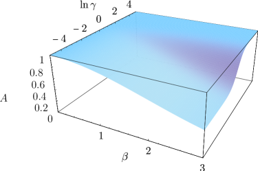
Figure 2: (Color online) Amplitude of the tunneling motion for $t\gg\Gamma^{-1}$ for $\eta=0$ as function of $\beta$ and $\ln\gamma$.

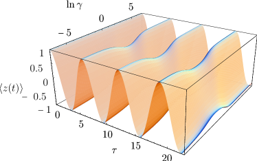
Figure 3: (Color online) Tunneling motion $\langle z(t)\rangle$ in units of $b/2$ as function of $\tau\equiv\Delta t$ and $\ln\gamma$ for $\beta=3$, $\eta=0$ with initial value $\langle z(0)\rangle=b/2$.

II.4 The electromagnetic field

We now calculate the electromagnetic field in the limit of large times, $t\gg\Gamma_{\pm}^{-1}$, such that the atom has emitted a photon with certainty. We will approximate again $\Gamma_{+}\simeq\Gamma_{-}\simeq\Gamma(\omega_{0})\equiv\Gamma$ (we are restricted to the regime $\omega_{0}\gg\Delta,\Gamma$). The wave function of the entire system has then the form

$$|\psi(\infty)\rangle=\sum_{k}\big{(}c_{1_{k}-g}(\infty)|1_{k}-g\rangle+c_{1_{k}+g}(\infty)|1_{k}+g\rangle\big{)}$$ (46)

with

$$c_{1_{k}\pm g}(\infty)=g_{k}\left(\frac{c_{{\bf 0}\pm e}(0)\cos\kappa}{\omega_{k}-\omega_{0}+i\Gamma/2}-i\>\frac{c_{{\bf 0}\mp e}(0)\sin\kappa}{\omega_{k}-\omega_{0}\pm\Delta+i\Gamma/2}\right)$$ (47)

(see (37)). The first order correlation function of the electric field $G^{(1)}(\mathbf{r},\mathbf{r};t,t)$ Scully and Zubairy (1997) is given for large times by

$$G^{(1)}(\mathbf{r},\mathbf{r};t,t) = \langle\psi(\infty)|{\bf E}^{(-)}(\mathbf{r},t).{\bf E}^{(+)}(\mathbf{r},t)|\psi(\infty)\rangle=|{\bf I}^{+}|^{2}+|{\bf I}^{-}|^{2}\,,$$ (48)

$${\bf I}^{\pm} = \sum_{k}c_{1_{k}\pm g}\langle 0|{\bf E}^{(+)}(\mathbf{r},t)|1_{k}\rangle\,,$$ (49)

with the positive frequency electric field operator ${\bf E}^{(+)}(\mathbf{r},t)=\sum_{k}{\cal E}_{k}\mbox{\boldmath{$\epsilon$}}_{k}a_{k}e^{i({\bf k}.{\bf r}-\omega_{k}t)}$. The difference between ${\bf I}^{+}$ and ${\bf I}^{-}$ rests upon $c_{1_{k}\pm g}$. We focus for the moment on ${\bf I}^{+}$. The corresponding results for ${\bf I}^{-}$ are obtained in a completely analogous fashion. In fact, according to Eqs. (47,49) one only needs to exchange $c_{{\bf 0}+e}\leftrightarrow c_{{\bf 0}-e}$ and replace $\Delta$ by $-\Delta$ in the final result to obtain ${\bf I}^{-}$ from ${\bf I}^{+}$. We choose the vector $\mathbf{r}$ to lie in the $x-z$ plane, convert the sum over $k$ into an integral as before, and are thus led to

$${\bf I}^{+} = -\frac{1}{16\pi^{3}\epsilon_{0}c^{3}}\int_{0}^{\pi}\sin\theta d\theta\int_{0}^{2\pi}d\phi\int_{0}^{+\infty}d\omega\omega^{3}\left(\bm{\wp}-\mathbf{k}\frac{\mathbf{k}.\bm{\wp}}{k^{2}}\right)e^{i(\mathbf{k}.\mathbf{r}-\omega t)}$$ (50)

$$\;\;\;\;\;\times\left(\frac{c_{{\bf 0}+e}(0)\cos\kappa}{\omega-\omega_{0}+i\Gamma/2}-i\>\frac{c_{{\bf 0}-e}(0)\sin\kappa}{\omega-\omega_{0}+\Delta+i\Gamma/2}\right)$$

$$= {\bf I}_{c}^{+}+{\bf I}_{s}^{+}\,,$$ (51)

where $\mathbf{k}.\mathbf{r}=(\omega/c)(z\cos\theta+x\sin\theta\cos\phi)$. The integral splits into two parts ${\bf I}_{c}^{+}$, ${\bf I}_{s}^{+}$ with denominators $\omega-\omega_{0}+i\Gamma/2$ and $\omega-\omega_{0}+\Delta+i\Gamma/2$. As in the Wigner-Weisskopf theory of spontaneous emission, we assume that $\omega^{3}$ varies little around $\omega=\omega_{0}$ (respectively $\omega=\omega_{0}-\Delta$) so that we can replace $\omega^{3}$ by $\omega_{0}^{3}$ (respectively $(\omega_{0}-\Delta)^{3}$) and extend the lower limit of integration to $-\infty$. Only the $x$ and $z$-components of ${\bf I}_{c}^{+}$ and ${\bf I}_{s}^{+}$, denoted as $I_{c,\xi}^{+}$ $I_{s,\xi}^{+}$, $\xi\in\{x,z\}$, give a contribution (the $y$-component is identically zero),

$$I_{c,\xi}^{+} = -\frac{\omega_{0}^{3}\wp\,c_{{\bf 0}+e}(0)}{16\pi^{3}c^{3}\epsilon_{0}}\int_{0}^{\pi}\sin\theta d\theta\int_{0}^{2\pi}d\phi\;f_{\xi}(\eta,\theta,\phi)$$ (52)

$$\times\int_{-\infty}^{+\infty}d\omega\frac{e^{i\omega(\frac{z}{c}\cos\theta+\frac{x}{c}\sin\theta\cos\phi-t)}\cos\left(\frac{\omega b}{2c}\cos\theta\right)}{\omega-\omega_{0}+i\Gamma/2}\,,$$

$$f_{x}(\eta,\theta,\phi) = [\sin\eta-\sin\theta\cos\phi(\sin\theta\cos\phi\sin\eta+\cos\theta\cos\eta)]\,,$$ (53)

$$f_{z}(\eta,\theta,\phi) = [\cos\eta-\cos\theta(\sin\theta\cos\phi\sin\eta+\cos\theta\cos\eta)]\,.$$ (54)

Writing $\cos\left(\frac{\omega b}{2c}\cos\theta\right)$ as a sum of exponentials, the $\omega$-integral can be easily evaluated using the contour method and leads to a Heaviside $\Theta$-function $\Theta\Big{(}t-((z\pm b/2)\cos\theta+x\sin\theta\cos\phi)/c\Big{)}$ for the positive (negative) frequency part of the $\cos\left(\frac{\omega b}{2c}\cos\theta\right)$ function, which illustrates the fact that the electric field cannot spread faster than the speed of light. In order to avoid the complications which arise from the angle dependence of the $\Theta$-function, we will restrict ourselves to times $t>\frac{1}{c}(r+b/2)$ with $r=\sqrt{x^{2}+z^{2}}$. We find

$$I_{c,\xi}^{+} = i\frac{\omega_{0}^{3}\wp\,c_{{\bf 0}+e}(0)}{8\pi^{2}c^{3}\epsilon_{0}}\int_{0}^{\pi}\sin\theta d\theta\int_{0}^{2\pi}d\phi\;f_{\xi}(\eta,\theta,\phi)$$

$$\;\;\;\;\;\times e^{i(\omega_{0}-i\Gamma/2)(\frac{z}{c}\cos\theta+\frac{x}{c}\sin\theta\cos\phi-t)}\cos\Big{(}\frac{b}{2c}(\omega_{0}-i\Gamma/2)\cos\theta\Big{)}\,.$$

Integration over the angle $\phi$ yields for the $x$-component

$$I_{c,x}^{+} = i\frac{\omega_{0}^{3}\wp\,c_{{\bf 0}+e}(0)}{4\pi c^{3}\epsilon_{0}}\int_{0}^{\pi}\sin\theta d\theta\;e^{i(\omega_{0}-i\Gamma/2)(\frac{z}{c}\cos\theta-t)}\cos\Big{(}\frac{b}{2c}(\omega_{0}-i\Gamma/2)\cos\theta\Big{)}$$ (56)

$$\times\Big{\{}\sin\eta\;J_{0}\left(\frac{x}{c}(\omega_{0}-i\Gamma/2)\sin\theta\right)-i\sin\theta\cos\theta\cos\eta\;J_{1}\left(\frac{x}{c}(\omega_{0}-i\Gamma/2)\sin\theta\right)$$

$$-\sin^{2}\theta\sin\eta\left[\frac{J_{1}\left(\frac{x}{c}(\omega_{0}-i\Gamma/2)\sin\theta\right)}{\frac{x}{c}(\omega_{0}-i\Gamma/2)\sin\theta}-J_{2}\left(\frac{x}{c}(\omega_{0}-i\Gamma/2)\sin\theta\right)\right]\Big{\}}\,,$$

where $J_{0}$, $J_{1}$, and $J_{2}$ are Bessel functions. A closed form of the type of the remaining $\theta$–integral has been found very recently by Neves et al. Neves et al. (2006). Using their formula, we can evaluate the $\theta$-integration analytically and find in the far-field region

$$I_{c,x}^{+} = i\frac{\omega_{0}^{3}\wp\,c_{{\bf 0}+e}(0)}{4\pi c^{3}\epsilon_{0}}\;e^{-i(\omega_{0}-i\Gamma/2)t}$$ (57)

$$\times\Big{\{}\sin\eta\;\left[\frac{\sin R_{+}}{R_{+}}+\frac{\sin R_{-}}{R_{-}}\right]-\sin\eta\left[\frac{\sin^{2}\alpha_{+}\sin R_{+}}{R_{+}}+\frac{\sin^{2}\alpha_{-}\sin R_{-}}{R_{-}}\right]$$

$$-\frac{1}{2}\cos\eta\;\left[\frac{\sin(2\alpha_{+})\sin R_{+}}{R_{+}}+\frac{\sin(2\alpha_{-})\sin R_{-}}{R_{-}}\right]\Big{\}}+\mathcal{O}(1/R_{\pm}^{2})\,,$$

with

$$R_{\pm}=\frac{(\omega_{0}-i\Gamma/2)}{c}\;r_{\pm}\,,$$ (58)

$$r_{\pm}=\sqrt{x^{2}+(z\pm b/2)^{2}}\,,$$

$$\tan\alpha_{\pm}=\frac{x}{z\pm b/2}\,.$$

The expression for $I_{c,z}^{+}$ is obtained from $I_{c,x}^{+}$ by a rotation of the coordinate system ($\eta\to\eta+\pi/2$, $\alpha_{\pm}\to\alpha_{\pm}+\pi/2$), which amounts in Eq. (57) to exchanging $\sin\eta\leftrightarrow\cos\eta$ and replacing $\sin^{2}\alpha_{\pm}\rightarrow\cos\alpha_{\pm}^{2}$. In the far-field, $\sin R_{\pm}\simeq e^{iR_{\pm}}/2i$, and the expressions can be further simplified,

$$I_{c,x}^{+} = \frac{\omega_{0}^{3}\wp\,c_{{\bf 0}+e}(0)}{8\pi c^{3}\epsilon_{0}}\;e^{-i(\omega_{0}-i\Gamma/2)t}$$ (59)

$$\times\Bigg{\{}\frac{e^{iR_{+}}}{R_{+}}\sin(\eta-\alpha_{+})\cos\alpha_{+}+\frac{e^{iR_{-}}}{R_{-}}\sin(\eta-\alpha_{-})\cos\alpha_{-}\Bigg{\}}+\mathcal{O}(1/R_{\pm}^{2})\,,$$

Similarly, we get for the second part $I_{s}^{+}$ of the integral

$$I_{s,x}^{+} = -\frac{(\omega_{0}-\Delta)^{3}\wp\,c_{{\bf 0}-e}(0)}{8\pi c^{3}\epsilon_{0}}\;e^{-i(\omega_{0}-\Delta-i\Gamma/2)t}$$ (60)

$$\times\Bigg{\{}\frac{e^{i\tilde{R}_{+}}}{\tilde{R}_{+}}\sin(\eta-\alpha_{+})\cos\alpha_{+}-\frac{e^{i\tilde{R}_{-}}}{\tilde{R}_{-}}\sin(\eta-\alpha_{-})\cos\alpha_{-}\Bigg{\}}+\mathcal{O}(1/\tilde{R}_{\pm}^{2})$$

with

$$\tilde{R}_{\pm}=\frac{(\omega_{0}-\Delta-i\Gamma/2)}{c}\;r_{\pm}\,.$$ (61)

The formulas for $I_{c,z}^{+}$ and $I_{s,z}^{+}$ are obtained by changing the global sign and replacing $\cos\alpha_{\pm}\rightarrow\sin\alpha_{\pm}$ where it appears explicitly in (59) and (60), respectively . We have

$$I_{c,x}^{+}+I_{s,x}^{+} \simeq\frac{\omega_{0}^{2}\wp}{8\pi c^{2}\epsilon_{0}}\frac{e^{-\frac{\Gamma}{2}(t-r/c)}}{r}\;e^{-i\omega_{0}t}$$ (62)

$$\;\;\;\;\;\times\Bigg{\{}c_{{\bf 0}+e}(0)\bigg{[}e^{i\frac{\omega_{0}}{c}r_{+}}\sin(\eta-\alpha_{+})\cos\alpha_{+}+e^{i\frac{\omega_{0}}{c}r_{-}}\sin(\eta-\alpha_{-})\cos\alpha_{-}\bigg{]}$$

$$\;\;\;\;\;-c_{{\bf 0}-e}(0)\>e^{i\Delta t}\bigg{[}e^{i\frac{(\omega_{0}-\Delta)}{c}r_{+}}\sin(\eta-\alpha_{+})\cos\alpha_{+}-e^{i\frac{(\omega_{0}-\Delta)}{c}r_{-}}\sin(\eta-\alpha_{-})\cos\alpha_{-}\bigg{]}\Bigg{\}}$$

$$\;\;\;\;\;+\mathcal{O}(\Delta/\omega_{0},\Gamma/\omega_{0},1/r^{2})\,,$$

and again the corresponding expression for $I_{c,z}^{+}+I_{s,z}^{+}$ can be found from Eq. (62) by just changing the global sign and the explicitly printed factors $\cos\alpha_{\pm}$ into $\sin\alpha_{\pm}$. We can summarize the results for both ${\bf I}^{+}$ and ${\bf I}^{-}$ as

$$|{\bf I}^{\pm}|^{2} = |I_{c,x}^{\pm}+I_{s,x}^{\pm}|^{2}+|I_{c,z}^{\pm}+I_{s,z}^{\pm}|^{2}$$

$$\simeq \frac{\omega_{0}^{4}\wp^{2}}{64\pi^{2}c^{4}\epsilon_{0}^{2}}\;\frac{e^{-\Gamma(t-r/c)}}{r^{2}}$$

$$\bigg{\{}\Big{|}c_{{\bf 0}\pm e}(0)\Big{[}e^{i\frac{\omega_{0}}{c}\delta r}\sin(\eta-\alpha_{+})\cos\alpha_{+}+\sin(\eta-\alpha_{-})\cos\alpha_{-}\Big{]}$$

$$-c_{{\bf 0}\mp e}(0)\>e^{\pm i\Delta(t-r_{-}/c)}\Big{[}e^{i\frac{(\omega_{0}\mp\Delta)\delta r}{c}}\sin(\eta-\alpha_{+})\cos\alpha_{+}-\sin(\eta-\alpha_{-})\cos\alpha_{-}\Big{]}\Big{|}^{2}$$

$$+\Big{|}c_{{\bf 0}\pm e}(0)\Big{[}e^{i\frac{\omega_{0}}{c}\delta r}\sin(\eta-\alpha_{+})\sin\alpha_{+}+\sin(\eta-\alpha_{-})\sin\alpha_{-}\Big{]}$$

$$-c_{{\bf 0}\mp e}(0)\>e^{\pm i\Delta(t-r_{-}/c)}\Big{[}e^{i\frac{(\omega_{0}\mp\Delta)\delta r}{c}}\sin(\eta-\alpha_{+})\sin\alpha_{+}-\sin(\eta-\alpha_{-})\sin\alpha_{-}\Big{]}\Big{|}^{2}$$

$$+\mathcal{O}(\Delta/\omega_{0},\Gamma/\omega_{0},1/r^{2})\bigg{\}}$$

with $\delta r=r_{+}-r_{-}$. In the limit $b\to 0$, we have $\delta r=0$, $\alpha_{\pm}=\alpha$ with $\tan\alpha=x/z$, and we recover the well-known result Scully et al. (1994) (valid for $t>r/c$)

$$G^{(1)}(\mathbf{r},\mathbf{r};t,t) =\frac{\omega_{0}^{4}\wp^{2}}{16\pi^{2}c^{4}\epsilon_{0}^{2}}\;\frac{e^{-\Gamma(t-r/c)}}{r^{2}}\;\sin^{2}(\eta-\alpha)\left(1+\mathcal{O}(\Delta/\omega_{0},\Gamma/\omega_{0},1/r^{2})\right)$$ (64)

where $\eta-\alpha$ is the angle between the dipole moment and the observer.

Using $\delta r\simeq b\cos\alpha$, $\cos\alpha_{\pm}\simeq\cos\alpha-\delta\alpha_{\pm}\sin\alpha$ and $\sin\alpha_{\pm}\simeq\sin\alpha+\delta\alpha_{\pm}\cos\alpha$ with $\delta\alpha_{\pm}=\alpha_{\pm}-\alpha\simeq\mp\frac{b}{2r}\sin\alpha$ in the far-field, we get for an initial delocalized state, $c_{{\bf 0}\pm e}(0)=1$ and $c_{{\bf 0}\mp e}(0)=0$,

$$G^{(1)}(\mathbf{r},\mathbf{r};t,t) \simeq\frac{\omega_{0}^{4}\wp^{2}}{16\pi^{2}c^{4}\epsilon_{0}^{2}}\;\frac{e^{-\Gamma(t-r/c)}}{r^{2}}\;\sin^{2}(\eta-\alpha)$$ (65)

$$\;\;\;\;\;\times\left[1\pm\sin\Big{(}\frac{\Delta b}{2c}\cos\alpha\Big{)}\sin\Big{(}\Big{[}\beta\pm\frac{\Delta b}{2c}\Big{]}\cos\alpha\Big{)}\right]$$

$$\;\;\;\;\;\times\left(1+\mathcal{O}(\Delta/\omega_{0},\Gamma/\omega_{0},1/r^{2})\right)\,,$$

where upper and lower sign now refer to the initial condition.

If the atom is initially located in the right well, $c_{{\bf 0}+e}(0)=c_{{\bf 0}-e}(0)=1/\sqrt{2}$ and we find

$$G^{(1)}(\mathbf{r},\mathbf{r};t,t) \simeq\frac{\omega_{0}^{4}\wp^{2}}{16\pi^{2}c^{4}\epsilon_{0}^{2}}\;\frac{e^{-\Gamma(t-r/c)}}{r^{2}}\;\sin^{2}(\eta-\alpha)$$ (66)

$$\;\;\;\;\;\times\left[1+\sin\Big{(}\frac{\Delta b}{2c}\cos\alpha\Big{)}\bigg{\{}\cos\big{(}\beta\cos\alpha\big{)}\sin\Big{(}\frac{\Delta b}{2c}\cos\alpha\Big{)}\right.$$

$$\left.\;\;\;\;\;\;\;\;\;\;\;-\sin\Big{(}\Delta\left[t-\frac{r}{c}\right]\Big{)}\bigg{(}1+\cos\big{(}\beta\cos\alpha\big{)}\bigg{)}\bigg{\}}\right]$$

$$\;\;\;\;\;\times\left(1+\mathcal{O}(\Delta/\omega_{0},\Gamma/\omega_{0},1/r^{2})\right)\,.$$

In both cases the interference term is proportional to $\sin\Big{(}\frac{\Delta b}{2c}\cos\alpha\Big{)}$ which scales in the non relativistic limit as $\Delta b/c$ and is thus extremely small.

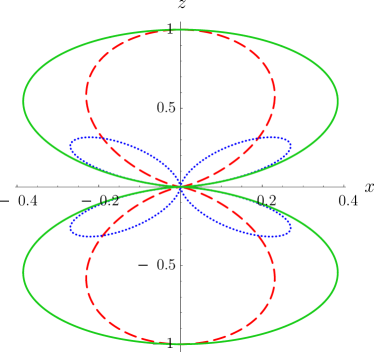
Figure 4: (Color online) Polar plot of $G^{(1)}_{\pm}(\mathbf{r},\mathbf{r};t,t)$ (red dashed and blue dotted curves) and $G^{(1)}(\mathbf{r},\mathbf{r};t,t)=G^{(1)}_{+}(\mathbf{r},\mathbf{r};t,t)+G^{(1)}_{-}(\mathbf{r},\mathbf{r};t,t)$ (green solid curve) for $\beta=3$, $\eta=0$, and an initially delocalized state $c_{{\bf 0}+e}(0)=1$.

The radiation from a classical oscillating dipole was examined recently by Bolotovskii and Serov Bolotovskii and Serov (2007). They predict interference effects in the regime where $\beta\simeq 1$, but do not provide any analytical results for the visibility of the interference fringes. It appears, however, that a classically moving dipole has to move a distance comparable to the wavelength during the time $1/\omega_{0}$ if waves from different origins are to combine in a remote location - otherwise the radiation pattern only follows its source adiabatically. Indeed, it is easy to show that at order zero in $\Delta b/c$ a classical oscillating dipole does not lead to interference (where $\Delta$ means now the classical oscillation frequency of the center–of–mass motion of the dipole). Therefore, the absence of interference in Eq. (66) at lowest order in $\Delta b/c$ agrees with the classical result. The initially delocalized states $|\pm\rangle$ do not have a classical analogue.

However, it turns out that in the quantum case interference with perfect visibility arises if the external state of the atom is post-selected in the energy basis. For example, if only runs of the experiments are taken into account where the atom is measured in external state $|+\rangle$ before the photon is recorded, only $|{\bf I}^{+}|^{2}$ (but not $|{\bf I}^{-}|^{2}$) contributes to $G^{(1)}(\mathbf{r},\mathbf{r};t,t)$. We find in this case $G^{(1)}_{+}(\mathbf{r},\mathbf{r};t,t)\propto\cos^{2}(\frac{\beta}{2}\cos\alpha)\sin^{2}(\eta-\alpha)$ (subscript $+$ for post-selection in $|+\rangle$). The interference fringes for post-selection in $|-\rangle$ are phase shifted, i.e., $G^{(1)}_{-}(\mathbf{r},\mathbf{r};t,t)\propto\sin^{2}(\frac{\beta}{2}\cos\alpha)\sin^{2}(\eta-\alpha)$, such that in the sum $G^{(1)}(\mathbf{r},\mathbf{r};t,t)=G^{(1)}_{+}(\mathbf{r},\mathbf{r};t,t)+G^{(1)}_{-}(\mathbf{r},\mathbf{r};t,t)$ the interference terms compensate and only the dipole characteristics $G^{(1)}(\mathbf{r},\mathbf{r};t,t)\propto\sin^{2}(\eta-\alpha)$ is left (see Fig. 4 for $\eta=0$). Note that for post-selection the interference pattern becomes independent of $\Delta$ and should therefore be observable even for small $\Delta$, as long as the two states can be reliably distinguished.

II.5 Experimental perspectives

Several requirements have to be met to observe the effects predicted in this paper. First of all, one needs a double–well potential with tunable well-to-well separation and barrier height in order to vary $b$ and $\Delta$. This has been demonstrated with optical dipole traps e.g. in Shin et al. (2004); Sebby-Strabley et al. (2006), and on atom chips e.g. in Hinds et al. (2001); Hänsel et al. (2001). Secondly, we considered in our model the same external potential for both internal states $|g\rangle$ and $|e\rangle$, and these states should be coupled by a dipole transition. It is by now well–known that this requirement can be met for Cs, Yb, Sr, and possibly Mg and Ca atoms at certain “magical wavelengths” in optical traps McKeever et al. (2003); Katori et al. (2003); Brusch et al. (2006); Barber et al. (2006). Thirdly, we made the two-level approximation for the external degree of freedom. It turns out that in a typical double–well potential at the limit of the Lamb-Dicke regime, $\beta\sim 3$ (i.e. $\lambda\sim 2b$) still leads to a reasonable restriction of the dynamics to the two lowest states. To show this, let us consider the usual quartic double–well potential $V(x)=V_{0}(z^{2}-a^{2})^{2}/a^{4}$ where $2a$ is the well-to-well separation. Similar results are obtained for other shapes of the double–well potential. The transition probability during emission of a photon between energy eigenstates $|n\rangle$ and $|m\rangle$ of this potential is given by $|\langle n|e^{ikz}|m\rangle|^{2}$ Cohen-Tannoudji et al. (2001). For Cs atoms and for the parameters $V_{0}=0.23$ MHz and $a=\lambda/4$, where $\lambda=852.4$ nm is the $6S_{1/2}\to 6P_{3/2}$ transition wavelength, this gives less than $10\%$ transition probability out of the ground state doublet with a tunneling splitting $\Delta\simeq 150$ Hz and $\beta\simeq 2.93$. For lighter atoms, such as Mg, tunnel splittings of the order of kHz can be easily achieved for the same $\beta$. The theory thus works well for $\beta\lesssim 3$ but not anymore for larger values. Equation (26) implies that for a $\Delta$ in the kHz range, $\Gamma\sim\Delta$ for a transition in the near-infrared ($\omega_{0}\sim 10^{13}$Hz), where a well-to-well separation of $\sim\mu$m leads to $\beta\sim 3$, which still keeps transition probabilities to higher vibrational states at less than about 10$\%$.

In any case, for optical traps the trap frequency and thus the tunnel splitting are determined by the laser power and the focusing (or the wavelength for optical lattices), and can therefore be controlled independently of $\Gamma$ such that both regimes $\Delta\gg\Gamma$ and $\Delta\ll\Gamma$ should be achievable. The spontaneous emission rate $\Gamma$ can be varied over a large interval by using a small static magnetic field to enable electrical dipole transitions between hyperfine levels that would otherwise be forbidden, due to admixture of small amplitudes of other hyperfine levels with allowed dipole transition Taichenachev et al. (2006); Mannervik et al. (1996).

Cooling close to the ground state in a single well trap has been demonstrated and should work down to temperatures $k_{B}T<\hbar\Delta$ if $\Delta$ is comparable to the single well vibrational frequency McKeever et al. (2003). Finally, one needs to detect the tunneling motion. That should be possible by optical imaging, i.e. diffusion of laser light from another transition in the optical regime with smaller wavelength than the well separation. Another possibility might be using the atomic spin as a position meter Haycock et al. (2000).

III Conclusions

A two–level atom which can tunnel between the two wells of a double–well potential allows for a host of interesting phenomena, which we have studied systematically in this paper in the regime $\delta=\Delta/\omega_{0}\ll 1$ (tunnel frequency much smaller than the atomic transition frequency) and $\beta=\omega_{0}b/c\lesssim 3$. Whereas the spontaneous emission rate $\Gamma$ of the atom is only slightly modified by putting the atom into a coherent symmetric superposition (ground state of the external double–well potential) of the two states in the right and left well, the tunneling of the atom and the properties of the emitted light are altered more profoundly. The emission of a single photon can cause decoherence of the tunneling motion, but only if 1.) the photon wavelength is not much larger than the distance between the two potential wells, and 2.) spontaneous emission is not too fast, i.e. $\Gamma\lesssim\Delta$. For $\Gamma\gg\Delta$, the photon is emitted even before the atom starts its tunneling motion, i.e. before a coherent superposition of eigenstates of the center–of–mass coordinate of the atom is established. Hence, despite strong coupling to the environment, the tunneling motion does not suffer from decoherence at all in this regime. After the emission of the photon no more decoherence takes place, and tunneling will then continue with constant amplitude. For very slow spontaneous emission, $\Gamma\ll\Delta$, the average amplitude of the tunneling motion reduces by a factor 2. The electric field of the emitted photon shows interference fringes, but their amplitude is very small unless the external state of the atom is post-selected in the energy basis, in which case interference fringes with perfect visibility arise. This is very reminiscent of the results in Schomerus et al. (2002), where it was predicted that interference fringes from the scattering of a particle by a quantum scatterer disappear in the limit where the kinetic energy $\epsilon\ll\Delta$, but can be recovered by post-selecting the elastic scattering channel. The effects predicted here should in principle be observable with modern cold–atom technology.

Acknowledgments: We would like to thank CALMIP (Toulouse) for the use of their computers. This work was supported by the Agence National de la Recherche (ANR), project INFOSYSQQ, and the EC IST-FET project EUROSQIP.

References

- Lenz and Meystre (1993) G. Lenz and P. Meystre, Phys. Rev. A 48, 3365 (1993).
- Eichmann et al. (1993) U. Eichmann, J. C. Bergquist, J. J. Bollinger, J. M. Gilligan, W. M. Itano, D. J. Wineland, and M. G. Raizen, Phys. Rev. Lett. 70, 2359 (1993).
- Itano et al. (1998) W. M. Itano, J. C. Bergquist, J. J. Bollinger, D. J. Wineland, U. Eichmann, and M. G. Raizen, Phys. Rev. A 57, 4176 (1998).
- Agarwal et al. (2002) G. S. Agarwal, J. von Zanthier, C. Skornia, and H. Walther, Phys. Rev. A 65, 053826 (2002).
- Feagin (2006) J. M. Feagin, Physical Review A (Atomic, Molecular, and Optical Physics) 73, 022108 (2006).
- Wickles and Müller (2006) C. Wickles and C. Müller, Europhys. Lett. 74, 240 (2006).
- Sebby-Strabley et al. (2006) J. Sebby-Strabley, M. Anderlini, P. S. Jessen, and J. V. Porto, Phys. Rev. A 73, 033605 (2006).
- Shin et al. (2004) Y. Shin, M. Saba, T. A. Pasquini, W. Ketterle, D. E. Pritchard, and A. E. Leanhardt, Phys. Rev. Lett. 92, 050405 (2004).
- Hänsel et al. (2001) W. Hänsel, J. Reichel, P. Hommelhoff, and T. W. Hänsch, Phys. Rev. A 64, 063607 (2001).
- Treutlein et al. (2006) P. Treutlein, T. W. Hansch, J. Reichel, A. Negretti, M. A. Cirone, and T. Calarco, Physical Review A (Atomic, Molecular, and Optical Physics) 74, 022312 (2006).
- Carnal and Mlynek (1991) O. Carnal and J. Mlynek, Phys. Rev. Lett. 66, 2689 (1991).
- Keith et al. (1991) D. W. Keith, C. R. Ekstrom, Q. A. Turchette, and D. E. Pritchard, Phys. Rev. Lett. 66, 2693 (1991).
- Hackermüller et al. (2004) L. Hackermüller, K. Hornberger, B. Brezger, A. Zeilinger, and M. Arndt, Nature 427, 711 (2004).
- Miffre et al. (2006) A. Miffre, M. Jacquey, M. Büchner, G. Trénec, and J. Vigué, Phys. Scr. 74, C15 (2006).
- Monroe et al. (1996) C. Monroe, D. M. Meekho, B. E. King, and D. J. Wineland, Science 272, 1131 (1996).
- Cohen-Tannoudji et al. (1992) C. Cohen-Tannoudji, F. Bardou, and A. Aspect (World Scientific, Singapore, 1992), Laser Sepectroscopy X.
- Rohrlich et al. (2006) D. Rohrlich, Y. Neiman, Y. Japha, and R. Folman, Phys. Rev. Lett. 96, 173601 (2006).
- Schomerus et al. (2002) H. Schomerus, Y. Noat, J. Dalibard, and C. W. J. Beenakker, Europhys. Lett. 57, 651 (2002).
- Japha and Kurizki (1996) Y. Japha and G. Kurizki, Phys. Rev. Lett. 77, 2909 (1996).
- (20) J. Martin and D. Braun, eprint quant-ph/0704.0763.
- Weisskopf and Wigner (1930) V. Weisskopf and E. Wigner, Z. Phys. 63, 54 (1930).
- Scully and Zubairy (1997) M. Scully and M. Zubairy, Quantum Optics (Cambridge University Press, Cambridge, UK, 1997).
- Berman (2005) P. R. Berman, Physical Review A (Atomic, Molecular, and Optical Physics) 72, 025804 (2005).
- Ankerhold et al. (1995) J. Ankerhold, H. Grabert, and G.-L. Ingold, Phys. Rev. E 51, 4267 (1995).
- Braun (2002) D. Braun, Phys. Rev. Lett. 89, 277901 (2002).
- Neves et al. (2006) A. A. R. Neves, L. A. Padilha, A. Fontes, E. Rodriguez, C. H. B. Curz, L. C. Barbosa, and C. L. Cesar, J. Phys. A: Math. Gen. 39, L293 (2006).
- Scully et al. (1994) M. O. Scully, H. Walther, and W. P. Schleich, Phys. Rev. A 49, 1562 (1994).
- Bolotovskii and Serov (2007) B. M. Bolotovskii and A. V. Serov, Bull. of the Lebedev Phys. Inst. 34, 73 (2007).
- Hinds et al. (2001) E. A. Hinds, C. J. Vale, and M. G. Boshier, Phys. Rev. Lett. 86, 1462 (2001).
- McKeever et al. (2003) J. McKeever, J. R. Buck, A. D. Boozer, A. Kuzmich, H.-C. Nägerl, D. M. Stamper-Kurn, and H. J. Kimble, Phys. Rev. Lett. 90, 133602 (2003).
- Katori et al. (2003) H. Katori, M. Takamoto, V. G. Pal’chikov, and V. D. Ovsiannikov, Phys. Rev. Lett. 91, 173005 (2003).
- Brusch et al. (2006) A. Brusch, R. L. Targat, X. Baillard, M. Fouche, and P. Lemonde, Physical Review Letters 96, 103003 (2006).
- Barber et al. (2006) Z. W. Barber, C. W. Hoyt, C. W. Oates, L. Hollberg, A. V. Taichenachev, and V. I. Yudin, Phys. Rev. Lett. 96, 083002 (2006).
- Cohen-Tannoudji et al. (2001) C. Cohen-Tannoudji, J. Dupont-Roc, and G. Grynberg, Processus d’interaction entre photons et atomes (EDP Sciences/CNRS Éditions, 75005 Paris, France, 2001).
- Taichenachev et al. (2006) A. V. Taichenachev, V. I. Yudin, C. W. Oates, C. W. Hoyt, Z. W. Barber, and L. Hollberg, Physical Review Letters 96, 083001 (2006).
- Mannervik et al. (1996) S. Mannervik, L. Broström, J. Lidberg, L.-O. Norlin, and P. Royen, Phys. Rev. Lett. 76, 3675 (1996).
- Haycock et al. (2000) D. L. Haycock, P. M. Alsing, I. H. Deutsch, J. Grondalski, and P. S. Jessen, Phys. Rev. Lett. 85, 3365 (2000).