Mean-field description of ultracold Bosons on disordered two-dimensional optical lattices

Abstract

In the present paper we describe the properties induced by disorder on an ultracold gas of Bosonic atoms loaded into a two-dimensional optical lattice with global confinement ensured by a parabolic potential. Our analysis is centered on the spatial distribution of the various phases, focusing particularly on the superfluid properties of the system as a function of external parameters and disorder amplitude. In particular, it is shown how disorder can suppress superfluidity, while partially preserving the system coherence.

In the last years, the experimental results concerning confined ultracold atoms in optical lattices have attracted much theoretical interest from many different fields, ranging from condensed-matter physics to quantum information theory (see e.g. A:Jaksch ; A:Calarco ). The ability of tuning the fundamental physical parameters has provided an unrivaled tool to devise specific physical situations which, beyond their intrinsic physical interest, can be employed as important simulation tools A:Jaksch . In particular, the possibility to engineer a defect-free periodic potential appears as one of the most intriguing characteristics of these systems. Such “cleanness” has allowed the experimental realization of the Bose-Hubbard (BH) model and the observation of the superfluid-Mott quantum phase transition discussed by Fisher in his seminal paper A:Fisher , where, in addition, the issue of the effect of disorder on the physical properties of the BH Hamiltonian was first addressed. Furthermore many experimental techniques such as laser speckle field A:Lye and the superposition of different optical lattices with incommensurate lattice constants A:Roth03 ; A:Damski2003 ; A:Fallani have recently substantiated the theoretical investigation of ultracold atoms in disordered optical lattices A:Krutitsky ; A:Yukalov , revealing a rich scenario of new physical situations such as the appearance of new phases (e.g. Bose-glass phase A:Damski2003 ; A:Fallani ) and superfluid (SF) percolation in $d$-dimensional ($d>1$) lattices A:Sheshadri1995 ; A:Ospelkaus .

In this paper we will deal with the properties of a two-dimensional (2D) optical lattice where bosons are confined by an overall parabolic potential and subject to a random potential distribution.

The experimental realization of 2D lattices is discussed in A:Greiner , A:Moritz and A:Spielman . In particular the latter represents a direct experimental realization of the Hamiltonian discussed in the present paper, when disorder is absent. A valuable feature of the setup here considered is the possibility to investigate a wide range of physical situations and geometries according to different external parameter choices. While the parabolic potential confines bosons in a disk-like domain, the interplay of the other external parameters (hopping amplitude and chemical potential), allows one to realize, for example, Mott phases distributed in concentric shells, each with different filling, intercalated with SF shells. The 1D counterpart of this scenario has been thoroughly studied in A:Batrouni2002 .

Here we will focus particularly on the superfluid-phase spatial distribution in the presence of a random potential. We analyze first the situation where a (single) central disk-like Mott region is surrounded by a thin SF shell, and then the case when the system is fully SF. We show that, in the first case, the quasi-1D SF domain is strongly influenced by the presence of “impurities”, leading to the drop of the SF fraction for a small increase of the disorder amplitude. In the second case, the genuine 2D geometry of the SF domain leads to the formation of circulating streams which do not disappear abruptly when the disorder amplitude is increased. In this respect our setup therefore appears to be an effective tool to investigate the combined effect of disorder and dimensionality on the SF properties of a bosonic system.

The system considered is modeled by a BH Hamiltonian $H=H_{I}+H_{T}$, with

$$H_{I}=\frac{U}{2}\sum_{i=1}^{M}n_{i}(n_{i}-1)-\sum_{i=1}^{M}\mu_{i}\,n_{i},\,\,H_{T}=-T\sum_{i,j}^{M}a_{i}^{\dagger}A_{ij}a_{j}+h.c.$$ (1)

where $n_{i}=a_{i}^{\dagger}a_{i}$, $a_{i}^{\dagger}$ ($a_{i}$) represents the creation (destruction) operator at site $i$, and the total boson number $N=\sum_{i}n_{i}$ is a conserved quantity. The random on-site effective chemical potential $\mu_{i}$ is given by

$$\mu_{i}=-\Omega_{0}(x_{i}^{2}+y_{i}^{2})+\Delta_{i}+\mu$$ (2)

accounting both for the noise distribution $\Delta$ ($\Delta_{i}=\Delta\cdot\xi_{i}$ with $\xi_{i}$ uniformly distributed between $0$ and $1$) and for the parabolic confinement $\Omega_{0}$. The Hamiltonian parameters $U$ and $T$ represent the two-body interaction and the hopping amplitude between neighboring sites respectively, $M$ is the total number of sites (in our simulations we have chosen $M=31^{2}=961$) and the matrix $A_{ij}$ is the so-called adjacency matrix, which is zero if sites $i$ and $j$ are not connected, and one otherwise.

Our analysis is based on the mean-field decoupling scheme already exploited by many authors for the analysis of the disordered BH model A:Damski2003 ; A:Sheshadri1995 ; A:Sheshadri1993 . For an application of this scheme to a disordered system see A:Buonsante06CM . Despite the well known shortcoming of not taking into account spatial correlations of quantum origin (see e.g. the discussion about spatial correlations in A:Wessel , and in particular Fig. 4 therein), this mean-field decoupling scheme has proven the ability to disclose and qualitatively characterize the prominent physical features of Bosonic atoms loaded in optical lattices, expecially in dimension greater than one (for a detailed discussion on the MF scheme and its application see A:Buonsante and references therein). Note however that we take into account the spatial dependence arising from the disordered+harmonic local potential, and hence — at least partially — the spatial correlations thereof. The essence of this approximation is the replacement of two-boson operators $a^{\dagger}_{i}a_{i^{\prime}}$ with single-site operators weighted by mean-field parameters $\alpha_{i}=\langle\psi|a_{i}|\psi\rangle$ (where $\alpha_{i}\in\mathbb{C}$ and $|\psi\rangle$ represents the mean-field ground state). Namely

$$a_{i}^{\dagger}a_{i^{\prime}}\approx a_{i}^{\dagger}\alpha_{i^{\prime}}+\alpha_{i}^{*}a_{i^{\prime}}-\alpha_{i}^{*}\alpha_{i^{\prime}}\quad\textrm{with }i\in\left[1,\dots,N\right]$$ (3)

where $\alpha_{i}$s have to be determined by self-consistency standard procedure.

Within this scheme, Hamiltonian $H$ can thus be approximated by $H\simeq\sum_{i}{\cal H}_{i}+h$ where $h=T\sum_{\ell=1}^{M}\alpha_{i}^{*}A_{i\,\ell}\alpha_{\ell}$ and parameters $\gamma_{i}=\sum_{\ell=1}^{M}A_{i\,\ell}\alpha_{\ell}$ in the single-site Hamiltonian ${\cal H}_{i}=Un_{i}(n_{i}-1)/2-\mu_{i}\,n_{i}-T(\gamma_{i}a_{i}^{\dagger}+\gamma_{i}^{*}a_{i})$ take into account the original inter-site coupling.

Most of the the fundamental physical properties of the system can be obtained from the values of $\alpha_{i}$ calculated from Hamiltonian $H$ alone where $T\in\mathbb{R}$. However, in order to properly describe the SF properties of the system it is well known that one has to go through same procedure with the introduction of the Peierls factors A:Shastry . The Hamiltonian with the addition of the Peierls factors reads

$$\tilde{H}=H_{I}+\tilde{H}_{T},\quad\tilde{H}_{T}=-T\sum_{i,j}\rme^{-i\theta B_{ij}}a_{i}^{\dagger}A_{ij}a_{j}+h.c.\,.$$ (4)

The quantity $\theta B_{ij}$ accounts for an infinitesimal velocity field $\mathbf{v}$ which can be considered as a “probe” to test the superfluidity properties of the system through the relation $\theta B_{ij}=m/\hbar\int_{\mathbf{r}_{i}}^{\mathbf{r}_{j}}\mathbf{v}\cdot d\mathbf{r}$ A:Wu where $\mathbf{r}_{i}$ is the $i$-th site position. With the Peierls factors $\tilde{H}$ becomes the Hamiltonian in the moving reference frame which is analogous to the Hamiltonian of a charged particle in presence of a magnetic field (see e.g. A:Wu ). For the determination of the response of the system, it is necessary to take the limit $\theta\to 0$ and hence it is appropriate to consider the presence of the Peierls factors in perturbative terms with respect to the Hamiltonian $H$. Up to first order, it is possible to show that the mean-field parameters for the Hamiltonian $\tilde{\mathcal{H}}$, corresponding through the mean-field site-decoupling approach to the Hamiltonian $\tilde{H}$, assume the following form $\alpha_{i}=\alpha^{0}_{i}\exp\left[-i\theta\phi_{i}\right]$, where $\alpha_{i}^{0}$ represent the (real) mean-field parameter related to the Hamiltonian $\mathcal{H}$, and the form of the phase term depends on the first order approximation in $\theta$.

In this paper we define the SF fraction (SFF) as the ratio between the current operator, as evaluated in Eq. (7), and the maximum possible SF current between two sites, i.e.

$$f_{\rm s}=\frac{\sum_{ij}\langle\psi|J_{ij}|\psi\rangle}{\sum_{ij}\langle\psi|J^{max}_{ij}|\psi\rangle}\quad\textrm{with }\quad\langle\psi|J^{max}_{ij}|\psi\rangle=-2T\sqrt{n_{i}}\sqrt{n_{j}}B_{ij}$$ (5)

where we have employed the current operator defined as

$$J_{ij}=iT\left(\exp[-i\theta B_{ij}]a_{j}^{\dagger}a_{i}-\exp[i\theta B_{ij}]a_{i}^{\dagger}a_{j}\right)$$ (6)

which describes the supercurrent in the rotating (lattice) frame. Recalling Eq. (3), the first-order approximation for the expectation value of the current operator can be written in the mean-field scheme as

$$\mathcal{J}_{ij}=\langle\psi|J_{ij}|\psi\rangle\simeq-2T\alpha^{0}_{i}\alpha^{0}_{j}\theta\left[\phi_{j}-\phi_{i}+B_{ij}\right].$$ (7)

So far, we have not explictly defined the structure of the site-dependent (through matrix $B_{ij}$) Peierls factors. As suggested by the circular symmetry of the parabolic potential, we have considered by definition $B_{ij}$ an infinitesimal rotation around the paraboloid axis. The generated flow –observed in the rotating frame– must be construed as a response to this infinitesimal rotation. To interpret correctly Figs. 1, 2, and 4, where the spatial distribution of $\mathcal{J}_{ij}$ is depicted, it necessary to recall that supercurrents are depicted in the (rotating) lattice frame and hence, in the laboratory frame, the overall rigid-body rotation effect must be subtracted. The SFF at rest appears thus to be surrounded by a rotating rigid-body – in this case the non-SF fraction.

In the 1D homogeneous case $f_{s}$ vanishes iff $\alpha_{i}=0$ (the standard condition for Mott regime). In this case, the translational invariance of the system holds, entailing $n_{i}=n_{j}=n$, $\alpha^{0}_{i}=\alpha^{0}_{j}=\alpha_{0}$ and $\phi_{i}=\phi_{j}$ (overall phase coherence), thus $\mathcal{J}_{ij}=0$ iff $\alpha_{0}=0$. In 2D disordered case, conversely, Eq. 7 shows that the condition $f_{s}=0$ is ensured either by $\alpha_{i}=0$, like in the 1D homogeneous case, or, more interestingly, by means of a phase rearrangement, which is determined by the constraint $\phi_{j}-\phi_{i}+B_{ij}=0$, entailing the emergence of local clusters with $\alpha_{i}\neq 0$.

It is worth noticing that, for a uniform ($\mu_{i}=\mu$) 1D system, due to translational invariance, Eq. (5) reproduces the mean-field behavior of SFF as defined in the literature A:Roth03b

$$f_{\rm s,1D}=\frac{\sum_{ij}2T\alpha_{0}^{2}B_{ij}}{\sum_{ij}2TnB_{ij}}=\frac{\alpha_{0}^{2}}{n}.$$ (8)

The identification of $f_{\rm s,1D}$ with $\alpha_{0}^{2}/n$ deserves some comments. In A:Penrose it was shown that the largest eigenvalue of the one-body density matrix $\rho_{ij}=\langle\psi|a^{\dagger}_{i}a_{j}|\psi\rangle/N$ is a measure of the condensate fraction $f_{c}$. Within the mean-field scheme, it is possible to prove that the ratio ${\langle\alpha_{i}^{2}\rangle}/{\langle n_{i}\rangle}$– the space average ${\langle x_{i}\rangle}$ ($x=\alpha,\,n$) takes into account the lattice inhomogeneity due to the disorder–, can be related to the largest eigenvalue of the mean-field approximation of matrix $\rho_{ij}=\left[\left(\langle\psi|n_{i}|\psi\rangle-|\alpha_{i}|^{2}\right)\delta_{ij}+\alpha^{*}_{i}\alpha_{j}\right]|/N$ and thus provides an estimate of the condensate fraction $f_{c}$. In this spirit, for a uniform system, Eq. (8) satisfies the condition $f_{c}\sim f_{s}$. From a more general point of view, since the condition $f_{c}\neq 0$ implies long range correlations, ${\langle\alpha_{i}^{2}\rangle}/{\langle n_{i}\rangle}$ can be viewed as a good coherence measure even for a disordered system.

In the numerical simulations we have analyzed two different situations. In the first case, we have evaluated the effect of noise on a configuration where a single central Mott domain, with $n_{i}=1$, is surrounded by a SF shell (Fig. 1), exhibiting a ring supercurrent. The parameters choice in this case has been performed in order to obtain a quasi-1D ring-shaped domain. In the laboratory frame the latter corresponds to inert matter decoupled from the lattice rotation owing to its SF character. This situation was explored in A:Wessel , in absence of disorderNota . In comparison, as a second case, we consider a situation where a central disk-like SF region is present and, consequently, exhibits a 2D behavior.

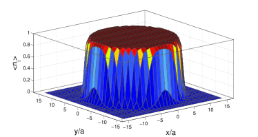
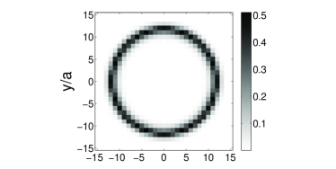
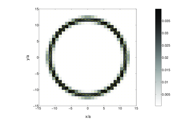
Figure 1: Upper Panels. Expectation value for the local number operator (left) and value of $\alpha_{i}$ (right). Lower Panel. Expectation value for the current operator $J_{ij}$. Both configurations are considered in absence of disorder

Case I.

In the first case ($T/U=1.6\,10^{-2}$, $\Omega_{0}/U=6\,10^{-3}$ and $\mu/U=0.5$ corresponding to $N_{tot}=199$ total particles) the increase of the noise amplitude leads to the “fracture” of the ring with $\alpha_{i}\neq 0$ and to the drop of the SFF, leading the rearrangement of the SF flow within the new potential pattern (Fig. 2).

In the idealized situation of a perfect 1D ring domain, the presence of an impurity cutting the ring is sufficient to determine a sudden drop to zero in the supercurrent induced by the velocity field. In the situation here depicted, due to the finite radial extent of the SF region such an impurity occupies an extended domain. In addition to this effect several vortices emerge which correspond to feeble supercurrents pinned around the sites with large (disorder-induced) local chemical potential $\mu_{i}$ (see Fig.2, lower panel).

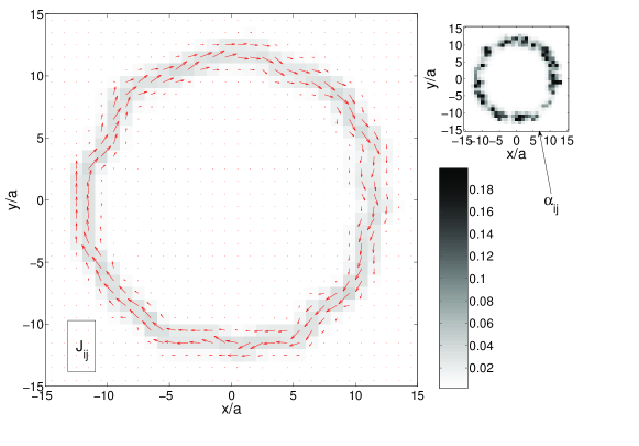
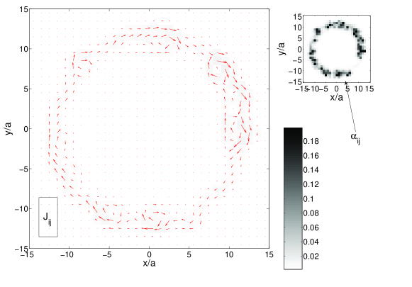
Figure 2: Effect of increasing noise amplitude on the flux $J_{ij}$ (arb. units) distribution (left) and on the $\alpha_{i}$ distribution (small panel, right). The figures considered represent noise amplitudes $\Delta/\Omega_{0}=$ 60 (top), 67 (bottom).

It is worth noticing that in the laboratory frame, the extended impurity rotates together with the pinned vortices dragged by the lattice.

The flow rearrangement in presence of disorder seems to be driven by the competition between the two terms in Eq. (7). In a situation where disorder is weak, the term $B_{ij}$ prevails, leading to a quasi-proportionality between the forcing term and the SF flow. On the other hand, in presence of large disorder, the phase pattern is adjusted so as to satisfy the condition $\phi_{j}-\phi_{i}\simeq-B_{ij}$. In this case the parameter $\langle\alpha_{i}^{2}\rangle/\langle n_{i}\rangle$, a good SFF measure for a homogeneous 1D system, while still being a measure of the local coherence of the system, can not be interpreted anymore as a measure of the SFF, since the presence of small clusters with $\alpha_{i}\neq 0$ will contribute to the overall $\langle\alpha_{i}^{2}\rangle/\langle n_{i}\rangle$ value but not to the SFF. Notice that here by “small” we refer to a three-site cluster, in that, in a 2D square lattice 4 sites are needed to close a loop and thus to support a current.

Fig. 3 shows that an increase of the disorder strength induces a sharp drop in the SFF while leaving the quantum coherence of the system almost unchanged. Each data point is the result of the average over 10 realizations of the random potential. For sake of clarity, the errorbars are plotted every fifth data point. As we discussed above, the sharp drop in the SFF corresponds to the interruption of the quasi 1D SF domain characterizing the system in the absence of disorder

A qualitative argument for the determination of the disorder-amplitude range in which the ring starts to break is to consider that, in the absence of disorder, the ring is approximately 2-sites thick and with a radius of about 12 sites. Hence the potential energy difference between radially adjacent sites is about $\Omega_{0}\cdot\left(12^{2}-11^{2}\right)$. In order to have superfluidity, the hopping must be large enough to overcome the potential difference $\Delta_{c}\simeq\Omega_{0}\cdot\left(12^{2}-11^{2}\right)$, where $\Delta_{c}$ can thus be viewed as the disorder amplitude corresponding to the drop in the SFF. As a consequence, if disorder-induced local potentials of up to the same amplitude are present, the SFF is not affected.

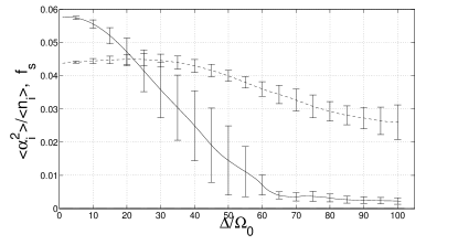
Figure 3: Comparison between the SFF (solid line) and the value of $\langle\alpha_{i}^{2}\rangle/\langle n_{i}\rangle$ (dashed line) as a function of disorder amplitude. Error bars account for the dispersion of the numerical data around their mean value for 10 different disorder realizations.

Case II.

The second setup has been conceived in order to analyze the effects of disorder in a fully 2D SF domain. In this case, due to the more markedly SF character of the system, it has been necessary to consider much larger noise amplitudes to have observable effects on the SF distribution. In Fig. 4 we have sketched the values for $\mathcal{J}_{ij}$ and $\alpha_{i}$ in a situation exhibiting a strong SF character ($T/U=0.1$, $\Omega_{0}/U=3.6\,10^{-2}$, $\mu/U=0.6$ with $N_{tot}=313$ ) for increasing values of the noise amplitude. Low values for $\mathcal{J}_{ij}$ on the lattice center are direct consequence of the velocity pattern imposed on the lattice and must not be interpreted as the absence of superfluidity at the center of the trap. As previously discussed, in this case we have $\mathcal{J}_{ij}\propto-B_{ij}$.

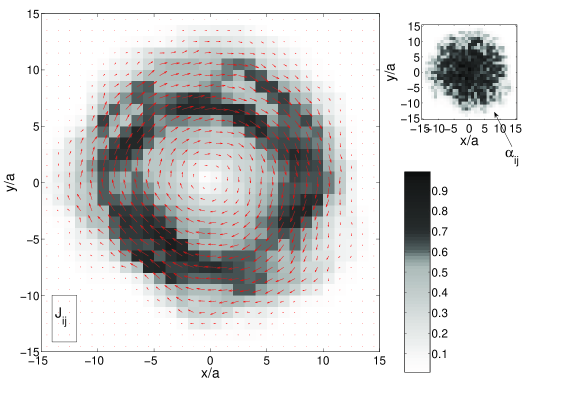
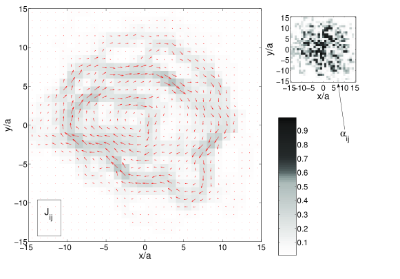
Figure 4: Effect of increasing noise amplitude on the flux $J_{ij}$ (arb. units) distribution (left) and on the $\alpha_{i}$ distribution (small panel, right). The figures considered represent disorder amplitudes $\Delta/\Omega_{0}=$ 200 (top), 600 (bottom).

For increasing values of the ratio between the noise and the parabola amplitude ( $\Delta/\Omega_{0}$ ), as in Case I, the SFF, due to the rearrangement of the flow, has a slower decrease than in the previous situation, due to the much larger SFF – note the scale difference between Fig. 3 and Fig. 5.

A prominent difference between Case I and Case II resides in the fact that the first one can be considered a quasi-1D case, and hence the “cutting” of the SF shell is analogous to the interruption of a 1D chain. The second case represents, on the other hand, a genuine 2D situation and, as it is possible to see in Fig. 4, the presence of noise leads to the formation of percolation patterns with nonzero circulation A:Sheshadri1995 . The supercurrents in this case will follow closed and possibly merging paths encircling domains characterized by $f_{s}=0$ but $\langle\alpha_{i}^{2}\rangle/\langle n_{i}\rangle\neq 0$. The latter shows then the survival of a local coherence character, connected to $f_{c}$, even in the absence of supercurrents. The condition $f_{c}\neq 0$ together with $f_{s}=0$, according to the scheme of Ref. A:Buonsante06CM , supplies, in the thermodynamical limit, a possible characterization of a Bose-glass phase.

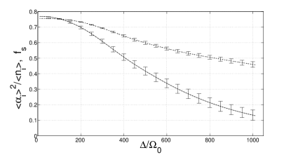
Figure 5: Comparison between the SFF (continuous line) and the value of $\langle\alpha_{i}^{2}\rangle/\langle n_{i}\rangle$ (dashed line) as a function of noise amplitude. Error bars account for the dispersion of the numerical data around their mean value for 10 different disorder realizations.

In conclusion, we have presented a theoretical study of the behavior of Bosonic ultracold atoms in a 2D optical lattice with parabolic radial confinement with disorder. Our investigation has focused on the SF response both in the weakly and in the strongly SF regime. Within our approximation scheme, we have shown that, in the 2D disordered case, the absence of supercurrents is determined by two independent effects: the (usual) vanishing of the parameters $\alpha_{i}$, and the phase rearrangement implied by $\phi_{j}-\phi_{i}+B_{ij}=0$. While the first effect can be related to the presence of a Mott phase in the thermodynamical limit, the second one, in the same limit, suggests the presence of a Bose-glass phase. In this framework, we have given a possible interpretation of the mechanism through which superfluidity is destroyed by disorder. Our numerical analysis evidences how, as a consequence of the phase rearrangement, the quasi-1D SF domain is destroyed by the appearance of “impurities”, with an ensuing drop of the SF fraction for a small increase of the disorder amplitude. Conversely, in Case II the genuine 2D nature of the SF domain leads to a multiple-stream SF flow determined by the increase of the disorder amplitude, with the consequent appearance of percolation patterns. In the laboratory frame, the strong-disorder sources in the rotating lattice have an overall site-dependent dragging effect on lattice bosons indicating the presence of non-superfluid regions locally surrounded by flows of nonzero circulation.

The rich phenomenology here presented exhibits a complex interplay between parameters such as the hopping amplitude, the boson-boson interaction, the disorder amplitude and the parabola coefficient. In view of the intrinsic interest from the experimental point of view, this deserves a more systematic analysis we will perform elsewhere.

References

- [1] D. Jaksch and P. Zoller. The cold atom Hubbard toolbox. Ann. Phys., 315:52, 2005.
- [2] T. Calarco, U. Dorner, P. S. Julienne, C. J. Williams, and P. Zoller. Quantum computations with atoms in optical lattices: Marker qubits and molecular interactions. Phys. Rev. A, 70(0123406), 2004.
- [3] M. P. A. Fisher, P. B. Weichman, G. Grinstein, and D. S. Fisher. Boson localization and the superfluid-insulator transition. Phys. Rev. B, 40:546, 1989.
- [4] J. E. Lye, L. Fallani, M. Modugno, D. S. Wiersma, C. Fort, and M. Inguscio. Bose-Einstein condensate in a random potential. Phys. Rev. Lett., 95:070401, 2005.
- [5] R. Roth. Phase diagram of bosonic atoms in two-color superlattices. Phys. Rev. A, 68:023604, 2003.
- [6] B. Damski, J. Zakrzewski, L. Santos, P. Zoller, and M. Lewenstein. Atomic bose and anderson glasses in optical lattices. Phys. Rev. Lett., 91:080403, 2003.
- [7] L. Fallani, J. E. Lye, V. Guarrera, C. Fort, and M. Inguscio. Onset of a bose-glass of ultracold atoms in a disordered crystal of light. cond-mat/0603655.
- [8] V.I. Yukalov, E.P. Yukalova, K.V. Krutitsky, R. Graham. Bose-Einstein-condensed gases in arbitrarily strong random potentials arXiv:0705.3768
- [9] V.I. Yukalov and R. Graham, Bose-Einstein-condensed systems in random potentials Phys. Rev. A, 75:023619, 2007.
- [10] K. Sheshadri, H. R. Krishnamurthy, R. Pandit, and T. V. Ramakrishnan. Percolation-enhanced localization in the disordered bosonic hubbard model. Phys. Rev. Lett., 75:4075, 1995.
- [11] S. Ospelkaus, C. Ospelkaus, O. Wille, M. Succo, P. Ernst, K. Sengstock, and K. Bongs. Localization of bosonic atoms by fermionic impurities in a three-dimensional optical lattice. Phys. Rev. Lett., 96:180403, 2006.
- [12] M. Greiner, I. Bloch, O. Mandel, T. W. Hansch, and T. Esslinger Exploring Phase Coherence in a 2D Lattice of Bose-Einstein Condensates. Phys. Rev. Lett., 87:160405, 2001.
- [13] H. Moritz , T. Stöferle, M. Köhl, and T. Esslinger Exciting Collective Oscillations in a Trapped 1D Gas. Phys. Rev. Lett., 91:250402, 2003.
- [14] I. B. Spielman, W. D. Phillips, and J. V. Porto. The Mott insulator transition in two dimensions cond-mat/0606216.
- [15] Batrouni G. G., Rousseau V., Scalettar R. T., Rigol M., Muramatsu A., Denteneer P. J. H., and Troyer M. Mott Domains of Bosons Confined on Optical Lattices. Phys. Rev. Lett., 89:117203, 2002.
- [16] K. Sheshadri, H. R. Krishnamurthy, R. Pandit, and T. V. Ramakrishnan. Superfluid and insulating phases in an interacting-boson model: mean-field theory and the RPA. Euorphys. Lett., 22, 1993.
- [17] P. Buonsante, V. Penna, A. Vezzani, and P.B. Blakie. Mean-field phase diagram of cold lattice bosons in disordered potentials. cond-mat/0610476, 2006.
- [18] S. Wessel, F. Alet, M. Troyer, and G. Batrouni. Quantum Monte Carlo simulations of confined bosonic atoms in optical lattices. Phys. Rev. A, 70:053615, 2004.
- [19] P. Buonsante, F. Massel, V. Penna, and A. Vezzani. Mean-field phase diagram for Bose-Hubbard Hamiltonians with random hopping Las. Phys. 17:538, 2007.
- [20] B.S. Shastry and B Sutherland. Twisted Boundary Conditions and Effective Mass in Heisenberg-Ising and Hubbard Rings. Phys. Rev. Lett., 65:243–246, 1990.
- [21] Congjun Wu, Han-Dong Chen, Jiang-Piang Hu, and Shou-Cheng Zhang. Vortex configurations of bosons in an optical lattice. Phys. Rev. A, 69:043609, 2004.
- [22] R. Roth and K. Burnett. Superfluidity and interference pattern of ultracold bosons in optical lattices. Phys. Rev. A, 67:031602(R), 2003.
- [23] O. Penrose and L. Onsager. Bose-Einstein condensation and liquid Helium. Phys. Rev., 104:576, 1956.
- [24] In order to corroborate the general validity of our method, we notice that the mean-field results in absence of disorder described in Fig. 1 seem to properly reproduce the main findings of the Quantum Mone Carlo approach of [18].