Post Common Envelope Binaries from SDSS. I: 101 white dwarf main sequence binaries with multiple SDSS spectroscopy

Abstract

We present a detailed analysis of 101 white dwarf-main sequence binaries (WDMS) from the Sloan Digital Sky Survey (SDSS) for which multiple SDSS spectra are available. We detect significant radial velocity variations in 18 WDMS, identifying them as post common envelope binaries (PCEBs) or strong PCEB candidates. Strict upper limits to the orbital periods are calculated, ranging from 0.43 to 7880 d. Given the sparse temporal sampling and relatively low spectral resolution of the SDSS spectra, our results imply a PCEB fraction of $\ga$15 % among the WDMS in the SDSS data base. Using a spectral decomposition/fitting technique we determined the white dwarf effective temperatures and surface gravities, masses, and secondary star spectral types for all WDMS in our sample. Two independent distance estimates are obtained from the flux scaling factors between the WDMS spectra, and the white dwarf models and main sequence star templates, respectively. Approximately one third of the systems in our sample show a significant discrepancy between the two distance estimates. In the majority of discrepant cases, the distance estimate based on the secondary star is too large. A possible explanation for this behaviour is that the secondary star spectral types that we determined from the SDSS spectra are systematically too early by 1–2 spectral classes. This behaviour could be explained by stellar activity, if covering a significant fraction of the star by cool dark spots will raise the temperature of the inter-spot regions. Finally, we discuss the selection effects of the WDMS sample provided by the SDSS project.

1 Introduction

A large fraction of all stars in the sky are part of binary or multiple systems (Iben, 1991). If the initial separation of the main-sequence binary is small enough, the more massive star will engulf its companion while evolving into a red giant, and the system enters a common envelope (CE, e.g. Livio & Soker 1988; Iben & Livio 1993). Friction within the CE leads to a rapid decrease of the binary separation and orbital period, and the energy and angular momentum extracted from the binary orbit eventually ejects the CE. Products of CE evolution include a wide range of important astronomical objects, such as e.g. high- and low-mass X-ray binaries, double degenerate white dwarf and neutron star binaries, cataclysmic variables and super-soft X-ray sources – with some of those objects evolving at later stages into type Ia supernova and short gamma-ray bursts. While the concept of CE evolution is simple, its details are poorly understood, and are typically described by parametrised models (Paczynski, 1976; Nelemans et al., 2000; Nelemans & Tout, 2005). Consequently, population models of all types of CE products are subject to substantial uncertainties.

Real progress in our understanding of close binary evolution is most likely to arise from the analysis of post common envelope binaries (PCEBs) that are both numerous and well-understood in terms of their stellar components – such as PCEBs containing a white dwarf and a main sequence star. While detailed population models are already available, (e.g. Willems & Kolb, 2004), there is a clear lack of observational constraints. Schreiber & Gänsicke (2003) showed that the sample of well-studied PCEBs is not only small, but being drawn mainly from “blue” quasar surveys, it is also heavily biased towards young systems with low-mass secondary stars – clearly not representative of the intrinsic PCEB population.

The Sloan Digital Sky Survey (SDSS) is currently providing the possibility of dramatically improving the observational side of PCEB studies, as it has already identified close to 1000 WDMS (see Fig. 1) with hundreds more to follow in future data releases (Raymond et al., 2003; Silvestri et al., 2006; Eisenstein et al., 2006; Southworth et al., 2007). Within SEGUE, a dedicated program to identify WDMS containing cold white dwarfs is successfully underway (Schreiber et al., 2007).

Identifying all PCEBs among the SDSS WDMS, and determining their binary parameters is a significant observational challenge. Here, we make use of SDSS spectroscopic repeat observations to identify 18 PCEBs and PCEB candidates from radial velocity variations, which are excellent systems for in-depth follow-up studies. The structure of the paper is as follows: we describe our WDMS sample and the methods used to determine radial velocities in Sect. 2. In Sect. 3 we determine the stellar parameters of the WDMS in our sample. In Sect. 4, we discuss the fraction of PCEBs found, the distribution of stellar parameters, compare our results to those of Raymond et al. (2003) and Silvestri et al. (2006), discuss the incidence of stellar activity on the secondary stars in WDMS, and outline the selection effects of SDSS regarding WDMS with different types of stellar components.

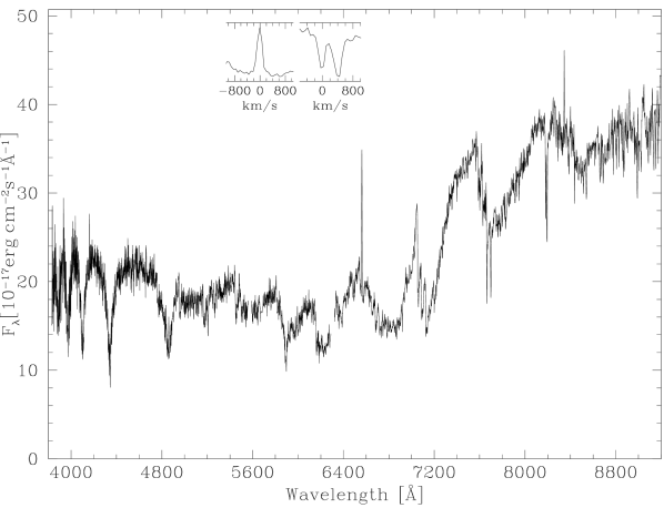
Figure 1: The spectrum of SDSS J005208.42-005134.6, a typical WDMS in the SDSS data base. The white dwarf is clearly visible in the blue while the low mass companion dominates the red part of the spectrum. Evident are the H$\alpha$ emission line, and the Na I $\lambda\lambda$ 8183.27,8194.81 absorption doublet, originating on the companion star. These features are shown in the small insets on a velocity scale, and are used to measure the radial velocities of 101 WDMS for which multiple SDSS spectra exist in DR5. See also Fig.  2.

2 Identifying PCEBs in SDSS

SDSS operates a custom-built 2.5 m telescope at Apache Point Observatory, New Mexico, to obtain $ugriz$ imaging with a 120-megapixel camera covering $1.5\,\mathrm{deg}^{2}$ at once. Based on colours and morphology, objects are then flagged for spectroscopic follow-up using a fibre-fed spectrograph. Each “spectral plate” refers physically to a metal plate with holes drilled at the positions of 640 spectroscopic plus calibration targets, covering $\sim 7\mathrm{deg}^{2}$. Technical details on SDSS are given by York et al. (2000) and Stoughton et al. (2002). The main aim of SDSS is the identification of galaxies (e.g. Strauss et al., 2002) and quasars (e.g. Adelman-McCarthy et al., 2006), with a small number of fibres set aside for other projects, e.g. finding cataclysmic variables and WDMS (Raymond et al., 2003).

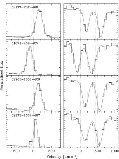
Figure 2: Fits to the Na I $\lambda\lambda$ 8183.27,8194.81 absorption doublet (right panels) and the H$\alpha$ emission line (left panels) in the four SDSS spectra of the WDMS SDSS J024642.55+004137.2. The SDSS spectroscopic identifiers (MJD, Plate-ID and Fibre-ID) are given in the top left corner of the H$\alpha$ panels. Na I has been fitted with a double-Gaussian of fixed separation plus a parabola, H$\alpha$ with a Gaussian plus a parabola. In this system, radial velocity variations are already obvious to the eye. The top three spectra are taken in a single night, the bottom one is combined from data taken on three nights, MJD = 52970, 52972, and 52973. The widths of the Gaussians fitting the Na I doublet are (top to bottom) 4.6 Å, 5.8 Å, 5.3 Å, and 6.0 Å.

A feature of SDSS hitherto unexplored in the study of WDMS is the fact that $\sim 10$ per cent of the spectroscopic SDSS objects are observed more than once: the detection of radial velocity variations between different SDSS spectra of a given WDMS will unambiguously identify such a system as a PCEB, or a strong PCEB candidate. Throughout this paper, we define a PCEB as a WDMS with an upper limit to its orbital period $\la 300$ d, a PCEB candidate as a WDMS with periods $300\,\mathrm{d}\la P_{\mathrm{orb}}\la 1500\,\mathrm{d}$, following Fig. 10 from Willems & Kolb (2004), which shows the period and mass distribution of the present-day WDMS population at the start of the WDMS binary phase. WDMS with period $\ga 1500$ d have too large binary separations to undergo a CE phase, and remain wide systems. While these definitions depend to some extend on the detailed configuration of the progenitor main sequence binary, the population model of Willems & Kolb (2004) predicts a rather clean dichotomy.

We have searched the DR5 spectroscopic data base for multiple exposures of all the WDMS listed by Silvestri et al. (2006) and Eisenstein et al. (2006), as well as a set of WDMS independently found in the SDSS data by our team. This search resulted in a sample of 130 WDMS with two to seven SDSS spectra. Among those WDMS, 101 systems have a clearly pronounced Na I $\lambda\lambda$ 8183.27,8194.81 absorption doublet and/or H$\alpha$ emission in their SDSS spectra, and were subjected to radial velocity measurements using one or both spectral features. The Na I doublet was fitted with a second order polynomial and double-Gaussian line profile of fixed separation. Free parameters were the amplitude and the width of each Gaussian and the velocity of the doublet. H$\alpha$ was fitted using a second order polynomial plus a single Gaussian of free velocity, amplitude and width. We computed the total error on the radial velocities by quadratically adding the uncertainty in the zeropoint of the SDSS wavelength calibration ($10\,km\,s^{-1}$, Stoughton et al. 2002) and the error in the position of the Na II/H$\alpha$ lines determined from the Gaussian fits. Figure 2 shows the fits to the four SDSS spectra of SDSS J024642.55+004137.2, a WDMS displaying an extremely large radial velocity variation identifying it as a definite PCEB. This figure also illustrates an issue encountered for a handful of systems, i.e. that the H$\alpha$ and Na I radial velocities do not agree in the latest spectrum (Table 1). This is probably related to the inhomogeneous distribution of the H$\alpha$ emission over the surface of the companion star, and will be discussed in more detail in Sect. 4.1. In total, 18 WDMS show radial velocity variations among their SDSS spectra at a $3\sigma$ level and qualify as PCEBs or strong PCEB candidates. Their radial velocities are listed in Table 1 and illustrated in Fig. 4 and Fig. 4. Three systems (SDSS0251–0000, SDSS1737+5403, and SDSS2345–0014) are subject to systematic uncertainties in their radial velocities due to the rather poor spectroscopic data. The radial velocities for the remaining 83 WDMS that did not show any significant variation are available in the electronic edition of the paper (see Table 2).

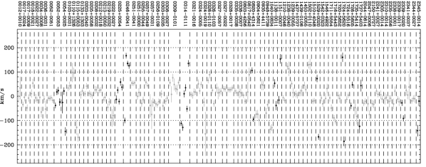
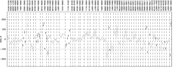
Figure 3: Radial velocities obtained from the Na I absorption doublet. WDMS $\geq 3\sigma$ RVs variation, i.e. PCEBs, are shown in black.

Figure 4: Same as Fig. 4 but for the H$\alpha$ radial velocities.

We note that special care needs to be taken in establishing the date and time when the SDSS spectra where obtained: a significant fraction of SDSS spectra are combined from observations taken on different nights (which we will call “sub-spectra” in what follows) in which case the header keyword MJDLIST will be populated with more than one date. The headers of the SDSS data provide the exposure start and end times in International Atomic Time (TAI), and refer to the start of the first spectrum, and the end of the last spectrum. Hence, a meaningful time at mid-exposure can only be given for those SDSS spectra that were obtained in a single contiguous observation.

A crucial question is obviously how the fact that some of the spectra in our sample are actually combinations of data from several nights impacts our aim to identify PCEBs via radial velocity variations. To answer this question, we first consider wide WDMS that did not undergo a CE phase, i.e. binaries with orbital periods of $\ga$ years. For these systems, sub-spectra obtained over the course of several days will show no significant radial velocity variation, and combining them into a single spectrum will make no difference except of increasing the total signal-to-noise ratio (S/N). In contrast to this, for close binaries with periods of a few hours to a few days, sub-spectra taken on different nights will sample different orbital phases, and the combined SDSS spectrum will be a mean of those phases, weighted by the S/N of the individual sub-spectra. In extreme cases, e.g. sampling of the opposite quadrature phases, this may lead to smearing of the Na I doublet beyond recognition, or end up with a very broad H$\alpha$ line. This may in fact explain the absence / weakness of the Na I doublet in a number of WDMS where a strong Na I doublet would be expected on the basis of the spectral type of the companion. In most cases, however, the combined SDSS spectrum will represent an “effective” orbital phase, and comparing it to another SDSS spectrum, itself being combined or not, still provides a measure of orbital motion. We conclude that the main effect of the combined SDSS spectra is a decreased sensitivity to radial velocity variations due to averaging out some orbital phase information. Figure 2 shows an example of a combined spectrum (bottom panel), which contains indeed the broadest Na I lines among the four spectra of this WDMS.

In order to check the stability of the SDSS wavelength calibration between repeat observations, we selected a total of 85 F-type stars from the same spectral plates as our WDMS sample, and measured their radial velocities from the Ca II $\lambda\lambda$ 3933.67,3968.47 $H$ and $K$ doublet in an analogous fashion to the Na I measurement carried out for the WDMS. None of those stars exhibited a significant radial velocity variation, the maximum variation among all checked F-stars had a statistical significance of $1.5\sigma$. The mean of the radial velocity variations of these check stars was found to be $14.5\,\mathrm{km\,s^{-1}}$, consistent with the claimed $10\,\mathrm{km\,s^{-1}}$ accuracy of the zero-point of the wavelength calibration for the spectra from an individual spectroscopic plate (Stoughton et al., 2002). In short, this test confirms that the SDSS wavelength calibration is stable in time, and, as anticipated above that averaging sub-spectra does not introduce any spurious radial velocity shifts for sources that have no intrinsic radial velocity variation (as the check stars are equally subject to the issue of combining exposures from different nights into a single SDSS spectrum). We are hence confident that any significant radial velocity variation observed among the WDMS is intrinsic to the system.

Table 1: Radial velocities of our 18 PCEBs and PCEB candidates, measured from the H$\alpha$ emission line and/or the Na I $\lambda\lambda$ 8183.27,8194.81 absorption doublet. The HJDs for SDSS spectra that have been combined from exposures taken in several different nights (see Sect. 2) are set in italics. PCEB candidates with uncertain radial velocity measurements are indicated by colons preceding and trailing the object name. Upper limits of the orbital periods are also provided (Sect. 4.2). The two spectral components identified in the spectra are coded as follows. DA = white dwarf with clearly visible Balmer lines; DC = clearly visible blue continuum without noticeable structure; blx = weak blue excess; dM = M-dwarf.

SDSS J	HJD	RV(H$\alpha$) $\mathrm{km\,s^{-1}}$			RV(Na) $\mathrm{km\,s^{-1}}$			$P_{\mathrm{orb}}\mathrm{[d]}<$
0052–0053	2451812.3463	71.3	$\pm$	16.6	23.4	$\pm$	14.9	280
DA/dM	2451872.6216	11.0	$\pm$	12.0	18.0	$\pm$	12.7
	2451907.0834	-62.1	$\pm$	11.7	-37.7	$\pm$	11.6
	2452201.3308	-26.0	$\pm$	16.0	-23.8	$\pm$	14.9
0054–0025	2451812.3463				21.6	$\pm$	15.3	4
DA/dM	2451872.6216				-25.6	$\pm$	44.2
	2451907.0835				-144.7	$\pm$	17.2
0225+0054	2451817.3966	53.0	$\pm$	14.9	58.6	$\pm$	15.4	45
blx/dM	2451869.2588	-19.2	$\pm$	20.7	-21.6	$\pm$	11.6
	2451876.2404	37.5	$\pm$	22.4	25.3	$\pm$	12.4
	2451900.1605	-25.1	$\pm$	14.0	-12.8	$\pm$	17.0
	2452238.2698	27.9	$\pm$	22.3	37.4	$\pm$	12.8
0246+0041	2451871.2731	-95.5	$\pm$	10.2	-99.3	$\pm$	11.1	2.5
DA/dM	2452177.4531	163.1	$\pm$	10.3	167.2	$\pm$	11.3
	2452965.2607	140.7	$\pm$	10.8	135.3	$\pm$	11.0
	2452971.7468	64.0	$\pm$	10.5	125.7	$\pm$	11.3
:0251–0000:	2452174.4732	4.1	$\pm$	33.5	0.0	$\pm$	15.4	0.58
DA/dM	2452177.4530	-139.3	$\pm$	24.6	15.8	$\pm$	18.3
0309–0101	2451931.1241	44.8	$\pm$	13.2	31.5	$\pm$	13.7	153
DA/dM	2452203.4500	51.2	$\pm$	14.1	48.7	$\pm$	24.4
	2452235.2865	27.4	$\pm$	14.1	76.3	$\pm$	16.2
	2452250.2457	28.8	$\pm$	15.0	8.1	$\pm$	33.0
	2452254.2052	53.9	$\pm$	11.8	55.7	$\pm$	14.3
	2452258.2194	15.5	$\pm$	13.0	27.9	$\pm$	19.9
	2453383.6493	50.7	$\pm$	11.0	56.5	$\pm$	12.8
0314–0111	2451931.1242	-41.6	$\pm$	12.4	-51.7	$\pm$	12.4	1.1
DC/dM	2452202.3882	35.6	$\pm$	10.9	35.2	$\pm$	14.4

SDSS J	HJD	RV(H$\alpha$) $\mathrm{km\,s^{-1}}$			RV(Na) $\mathrm{km\,s^{-1}}$			$P_{\mathrm{orb}}\mathrm{[d]}<$
	2452235.2865	9.1	$\pm$	11.0	10.3	$\pm$	14.2
	2452250.2457	-49.8	$\pm$	12.2	-128.2	$\pm$	13.9
	2452254.2053	-66.7	$\pm$	12.8	-111.7	$\pm$	10.9
	2452258.2195	87.3	$\pm$	10.8	135.2	$\pm$	13.5
0820+4314	2451959.3074	118.3	$\pm$	11.4	106.3	$\pm$	11.5	2.4
DA/dM	2452206.9572	-107.8	$\pm$	11.2	-94.6	$\pm$	10.8
1138–0011	2451629.8523				53.5	$\pm$	16.9	35
DA/dM	2451658.2128				-38.1	$\pm$	18.6
1151–0007	2451662.1689				-15.8	$\pm$	15.1	4.4
DA/dM	2451943.4208				154.0	$\pm$	19.5
1529+0020	2451641.4617				73.0	$\pm$	14.8	0.96
DA/dM	2451989.4595				-167.2	$\pm$	11.8
1724+5620	2451812.6712	125.6	$\pm$	10.2	160.6	$\pm$	18.4	0.43
DA/dM	2451818.1149	108.3	$\pm$	11.1	-	$\pm$	-
	2451997.9806	-130.6	$\pm$	10.3	-185.5	$\pm$	20.1
1726+5605	2451812.6712	-44.3	$\pm$	16.7	-38.9	$\pm$	12.9	29
DA/dM	2451993.9805	46.6	$\pm$	14.6	47.3	$\pm$	12.5
:1737+5403:	2451816.1187				-123.5	$\pm$	28.6	6.6
DA/dM	2451999.4602				44.0	$\pm$	24.0
2241+0027	2453261.2749	9.1	$\pm$	17.9	22.0	$\pm$	12.4	7880
DA/dM	2452201.1311	-60.3	$\pm$	12.7	8.1	$\pm$	12.2
2339–0020	2453355.5822	-29.2	$\pm$	10.4	-27.1	$\pm$	12.3	120
DA/dM	2452525.3539	-93.6	$\pm$	12.3	-90.1	$\pm$	12.7
:2345-0014:	2452524.3379				-141.5	$\pm$	22.9	9.5
DA/dM	2453357.5821				-19.8	$\pm$	19.3
2350-0023	2451788.3516	-160.3	$\pm$	16.6				0.74
blx/dM	2452523.3410	154.4	$\pm$	31.3

Notes on individual systems. 0246+0041, 0314–0111, 2241+0027, 2339–0020: variable H$\alpha$ equivalent width (EW); 0251–0000: faint, weak H$\alpha$ emission with uncertain radial velocity measurements; 1737+5403, 2345–0014: very noisy spectrum; See additional notes in Table LABEL:t-pcebfit

Table 2: 83 WDMS in our sample that did not show a significant a significant radial velocity variation between their different SDSS spectra. The complete table is available in the electronic edition of the paper. The first column gives the SDSS object name, the second the HJD of the spectrum, in the third column we quote with $y$ and $n$ those spectra which are composed of subspectra taken in different nights, the fourth and fith columns provide the Na I $\lambda\lambda$ 8183.27,8194.81 absorption doublet and H$\alpha$ emission radial velocities, respectively. Blanck spaces indicate that no radial velocity measurement could be obtained.

Object	HJD	Sub.	RV(H$\alpha$) $\mathrm{km\,s^{-1}}$			RV(Na) $\mathrm{km\,s^{-1}}$
SDSSJ001247.18+001048.7	2452518.4219	y	0.4	$\pm$	26.0	25.6	$\pm$	13.8
SDSSJ001247.18+001048.7	2452519.3963	y	34.1	$\pm$	46.7	9.1	$\pm$	20.0
SDSSJ001726.63-002451.1	2452559.2853	y	-4.0	$\pm$	16.2	-34.3	$\pm$	10.2
SDSSJ001726.63-002451.2	2452518.4219	y	-34.1	$\pm$	11.5	-32.0	$\pm$	12.9
SDSSJ001749.24-000955.3	2451794.7902	n	-47.6	$\pm$	13.6	-44.3	$\pm$	15.7
SDSSJ001749.24-000955.3	2452518.4219	y	-7.3	$\pm$	14.9	-8.7	$\pm$	11.6
SDSSJ001855.19+002134.5	2451816.3001	y	54.2	$\pm$	17.6
SDSSJ001855.19+002134.5	2451892.5884	n	11.0	$\pm$	16.3

3 Stellar parameters

The spectroscopic data provided by the SDSS project are of sufficient quality to estimate the stellar parameters of the WDMS presented in this paper. For this purpose, we have developed a procedure which decomposes the WDMS spectrum into its white dwarf and main sequence star components, determines the spectral type of the companion by means of template fitting, and derives the white dwarf effective temperature ($T_{\mathrm{eff}}$) and surface gravity ($\log g$) from spectral model fitting. Assuming an empirical spectral type-radius relation for the secondary star and a mass-radius relation for the white dwarf, two independent distance estimates are calculated from the flux scaling factors of the template/model spectra.

In the following sections, we describe in more detail the spectral templates and models used in the decomposition and fitting, the method adopted to fit the white dwarf spectrum, our empirical spectral type-radius relation for the secondary stars, and the distance estimates derived from the fits.

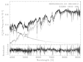
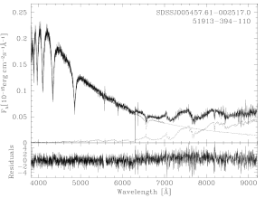
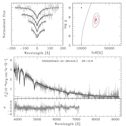
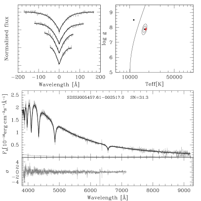
Figure 5: Two-component fits to the SDSS WDMS spectra. Shown are examples for objects with either the M-dwarf or the white dwarf dominating the SDSS spectrum. The top panels show the WDMS spectrum as black line, and the two templates, white dwarf and M-dwarf, as dotted lines. The bottom panels show the residuals from the fit. The SDSS spectrum identifies MJD, PLT and FIB are given in the plots below the object names.

Figure 6: Spectral model fits to the white dwarf components of the two WDMS shown in Fig.5, obtained after subtracting the best-fit M-dwarf template. Top left panels: best-fit (black lines) to the normalised H$\beta$ to H$\epsilon$ (gray lines, top to bottom) line profiles. Top right panels: 3, 5, and 10$\sigma$ $\chi^{2}$ contour plots in the $\mbox{$T_{\mathrm{eff}}$}-\log g$ plane. The black contours refer to the best line profile fit, the red contours to the fit of the whole spectrum. The dashed line indicates the occurrence of maximum H$\beta$ equivalent width. The best “hot” and “cold” line profile solutions are indicated by black dots, the best fit to the whole spectrum is indicated by a red dot. Bottom panels: the residual white dwarf spectra resulting from the spectral decomposition and their flux errors (gray lines) along with the best-fit white dwarf model (black line) to the 3850–7150 Å wavelength range (top) and the residuals of the fit (gray line, bottom). The $T_{\mathrm{eff}}$ and $\log g$ values listed in Table LABEL:t-pcebfit are determined from the best line profile fit. The fit to the whole spectrum is only used to select between the “hot” and “cold” line fit.

3.1 Spectral templates and models

In the course of decomposing/fitting the WDMS observations, we make use of a grid of observed M-dwarf templates, a grid of observed white dwarf templates, and a grid of white dwarf model spectra. High S/N ratio M-dwarf templates matching the spectral coverage and resolution of the WDMS data were produced from a few hundred late-type SDSS spectra from DR4. These spectra were classified using the M-dwarf templates of Beuermann et al. (1998). We averaged the $10-20$ best exposed spectra per spectral subtype. Finally, the spectra were scaled in flux to match the surface brightness at 7500 Å and in the TiO absorption band near 7165 Å, as defined by Beuermann (2006). Recently, Bochanski et al. (2007) published a library of late type stellar templates. A comparison between the two sets of M-dwarf templates did not reveal any significant difference. We also compiled a library of 490 high S/N DA white dwarf spectra from DR4 covering the entire observed range of $T_{\mathrm{eff}}$ and $\log g$. As white dwarfs are blue objects, their spectra suffer more from residual sky lines in the $I$-band. We have smoothed the white dwarf templates at wavelengths $>7000$ Å with a five-point box car to minimise the amount of noise added by the residual sky lines. Finally, we computed a grid of synthetic DA white dwarf spectra using the model atmosphere code described by Koester et al. (2005), covering $\log g=5.0-9.5$ in steps of 0.25 and $\mbox{$T_{\mathrm{eff}}$}=6000-100000$ K in 37 steps nearly equidistant in $\log(\mbox{$T_{\mathrm{eff}}$})$.

3.2 Spectral decomposition and typing of the secondary star

Our approach is a two-step procedure. In a first step, we fitted the WDMS spectra with a two-component model and determined the spectral type of the M-dwarf. Subsequently, we subtracted the best-fit M-dwarf, and fitted the residual white dwarf spectrum (Sect. 3.3). We used an evolution strategy (Rechenberg, 1994) to decompose the WDMS spectra into their two individual stellar components. In brief, this method optimises a fitness function, in this case a weighted $\chi^{2}$, and allows an easy implementation of additional constraints. Initially, we used the white dwarf model spectra and the M-dwarf templates as spectral grids. However, it turned out that the flux calibration of the SDSS spectra is least reliable near the blue end of the spectra, and correspondingly, in a number of cases the $\chi^{2}$ of the two-component fit was dominated by the poor match of the white dwarf model to the observed data at short wavelengths. As we are in this first step not yet interested in the detailed parameters of the white dwarf, but want to achieve the best possible fit of the M-dwarf, we decided to replace the white dwarf models by observed white dwarf templates. The large set of observed white dwarf templates, which are subject to the same observational issues as the WDMS spectra, provided in practically all cases a better match in the blue part of the WDMS spectrum. From the converged white dwarf plus dM template fit to each WDMS spectrum (see Fig. 5), we recorded the spectral type of the secondary star, as well as the flux scaling factor between the M-star template and the observed spectrum. The typical uncertainty in the spectral type of the secondary star is $\pm 0.5$ spectral class. The spectral types determined from the composite fits to each individual spectrum are listed in Table LABEL:t-pcebfit for the PCEBs in the analysed sample, and in the electronic edition of this paper for the remaining WDMS (see Table 4). Inspection of those tables shows that for the vast majority of systems, the fits to the individual spectra give consistent parameters. We restricted the white dwarf fits to WDMS containing a DA primary, consequently no white dwarf parameters are provided for those WDMS containing DB or DC white dwarfs.

3.3 White dwarf parameters

Once the best-fit M-dwarf template has been determined and scaled appropriately in flux, it is subtracted from the WDMS spectrum. The residual white dwarf spectrum is then fitted with the grid of DA models described in Sect. 3.1. Because of the uncertainties in the flux calibration of the SDSS spectra and the flux residuals from the M-star subtraction, we decided to fit the normalised H$\beta$ to H$\epsilon$ lines and omitted H$\alpha$ where the residual contamination from the secondary star was largest. While the sensitivity to the surface gravity increases for the higher Balmer lines (e.g. Kepler et al., 2006), we decided not to include them in the fit because of the deteriorating S/N and the unreliable flux calibration at the blue end. We determined the best-fit $T_{\mathrm{eff}}$ and $\log g$ from a bicubic spline interpolation to the $\chi^{2}$ values on the $\mbox{$T_{\mathrm{eff}}$}-\log g$ grid defined by our set of model spectra. The associated 1$\sigma$ errors were determined from projecting the contour at $\Delta\chi^{2}=1$ with respect to the $\chi^{2}$ of the best fit onto the $T_{\mathrm{eff}}$ and $\log g$ axes and averaging the resulting parameter range into a symmetric error bar.

The equivalent widths of the Balmer lines go through a maximum near $\mbox{$T_{\mathrm{eff}}$}=13\,000$ K, with the exact value being a function of $\log g$. Therefore, $T_{\mathrm{eff}}$ and $\log g$ determined from Balmer line profile fits are subject to an ambiguity, often referred to as “hot” and “cold” solutions, i.e. fits of similar quality can be achieved on either side of the temperature at which the maximum equivalent width is occurring. We measured the H$\beta$ equivalent width in all the model spectra within our grid, and fitted the dependence of the temperature at which the maximum equivalent width of H$\beta$ occurs by a second-order polynomial,

$$\mbox{$T_{\mathrm{eff}}$}(\mathrm{EW[H\beta]_{max}})=20361-3997\log g+390(\log g)^{2}$$ (1)

Parallel to the fits to the normalised line profiles, we fit the grid of model spectra to the white dwarf spectrum over the wavelength range $3850-7150$ Å (see Fig. 6). The red end of the SDSS spectra, where the distortion from the M-dwarf subtraction is strongest is excluded from the fit. We then use the $T_{\mathrm{eff}}$ and $\log g$ from the fits to the whole spectrum, continuum plus lines, to select the “hot” or “cold” solution from the line profile fits. In the majority of cases, the solution preferred by the fit to the whole spectrum has a substantially lower $\chi^{2}$ than the other solution, corroborating that it is likely to be the physically correct choice. In a few cases, the best-fit $T_{\mathrm{eff}}$ and $\log g$ from the whole spectrum are close to the maximum equivalent width given by Eq.1, so that the choice between the two line profile solutions is less well constrained. However, in most of those cases, the two solutions from the line profile fits overlap within their error bars, so that the final choice of $T_{\mathrm{eff}}$ and $\log g$ is not too badly affected.

Once that $T_{\mathrm{eff}}$ and $\log g$ are determined from the best line profile fit, we use an updated version of Bergeron et al.’s (1995) tables to calculate the mass and the radius of the white dwarf. Table LABEL:t-pcebfit reports $T_{\mathrm{eff}}$, $\log g$, and the white dwarf masses for the PCEBs in our sample, while the results for the remaining WDMS can be found in the electronic edition (Table 4). We have carefully inspected each individual composite fit, and each subsequent fit to the residual white dwarf spectrum, and are confident that we have selected the correct solution in the majority of cases. Some doubt remains primarily for a few spectra of very low signal-to-noise ratio. The fact that we have analysed at least two SDSS spectra for each system allows us to assess the robustness of our spectral decomposition/fitting method. Inspection of Table LABEL:t-pcebfit shows that the system parameter of a given system, as determined from several different SDSS spectra, generally agree well within the quoted errors, confirming that our error estimate is realistic.

3.4 An empirical spectral type-radius relation for M stars

Figure 7: Top panel: indirectly measured radii of M-dwarfs vs spectral type. Our empirical $Sp-R$ relation is given by a third order polynomial fit (solid line) to these data. Middle panel: mean radii and corresponding standard deviations obtained by averaging the radii in the top panel for each spectral type. Our $Sp-R$ relation is again superimposed. Bottom panel: directly measured radii of M-dwarfs, again our empirical $Sp-R$ relation, the dashed line is the theoretical $Sp-R$ relation from Baraffe et al. (1998). M-dwarf radii from the eclipsing WDMS RR Cae, NN Ser, DE CVn, RX J2130.6+4710 and EC 13471–1258 are shown as solid dots.

Sp	Rmean (R⊙)	Rσ (R⊙)	Rfit (R⊙)	Mfit (M⊙)	$T_{\mathrm{eff}}$ (K)
M0.0	0.543	0.066	0.490	0.472	3843
M0.5	0.528	0.083	0.488	0.471	3761
M1.0	0.429	0.094	0.480	0.464	3678
M1.5	0.443	0.115	0.465	0.450	3596
M2.0	0.468	0.106	0.445	0.431	3514
M2.5	0.422	0.013	0.420	0.407	3432
M3.0	0.415	0.077	0.391	0.380	3349
M3.5	0.361	0.065	0.359	0.350	3267
M4.0	0.342	0.096	0.326	0.319	3185
M4.5	0.265	0.043	0.292	0.287	3103
M5.0	0.261	0.132	0.258	0.255	3020
M5.5	0.193	0.046	0.226	0.225	2938
M6.0	0.228	0.090	0.195	0.196	2856
M6.5	0.120	0.005	0.168	0.170	2773
M7.0	0.178	0.080	0.145	0.149	2691
M7.5	0.118	0.009	0.126	0.132	2609
M8.0	0.137	0.046	0.114	0.120	2527
M8.5	0.110	0.004	0.109	0.116	2444
M9.0	0.108	0.004	0.112	0.118	2362
M9.5	0.111	0.008	0.124	0.130	2281

Table 3: Empirical $Sp-R$, $Sp-M$ and $Sp-\mbox{$T_{\mathrm{eff}}$}$ relations (R_fit, M_fit, $T_{\mathrm{eff}}$) found in this work. R_mean and R_σ represent the mean radii and their standard deviation obtained from the sample of M-dwarfs described in Sect. 3.4.

In order to use the flux scaling factor between the observed WDMS spectra and the best-fit M-dwarf templates for an estimate of the distance to the system (Sect. 3.5), it is necessary to assume a radius for the secondary star. Since we have determined the spectral types of the companion stars from the SDSS spectra (Sect. 3.2), we require a spectral type-radius relation ($Sp-R$) for M-dwarfs. The community working on cataclysmic variables has previously had interest in such a relation (e.g. Mateo et al., 1985; Caillault & Patterson, 1990), but while Baraffe & Chabrier (1996) derived theoretical mass/radius/effective temperature-spectral type relationships for single M-dwarfs, relatively little observational work along these lines has been carried out for field low mass stars. In contrast to this, the number of low mass stars with accurate mass and radius measurements has significantly increased over the past few years (see e.g. the review by Ribas, 2006), and it appears that for masses below the fully convective boundary stars follow the theoretical models by Baraffe et al. (1998) relatively well. However, for masses $\ga 0.3$ M_⊙, observed radii exceed the predicted ones. Stellar activity (e.g. López-Morales, 2007) or metallicity effects (e.g. Berger et al., 2006) were identified as possible causes.

Table 4: Stellar parameters of the remaining WDMS identified in our sample, as determined from spectral modelling. The complete table can be found in the electronic edition. Given are, from left to right: SDSS object name, MJD, fiber and plate number of the spectrum, white dwarf effective temperature and error, white dwarf surface gravity and error, mass of the white dwarf and error, distance to the white dwarf and error, spectral type of the secondary star, distance to the secondary and error, flag (we refer by and $s$ and $e$ those systems which have been studied previously by Silvestri et al. (2006) and Eisenstein et al. (2006), by $re$ those systems whose binary components are resolved), and notes.

Object	MJD	plate	fiber	T(k)	err	$\log g$	err	M(M⨀)	err	dwd(pc)	err	Sp	dsec(pc)	err	flag	notes
SDSSJ000442.00-002011.6	51791	387	24	-	-	-	-	-	-	-	-	0	2187	236	re	1
	52943	1539	21	-	-	-	-	-	-	-	-	0	2330	251
SDSSJ001029.87+003126.2	51793	388	545	-	-	-	-	-	-	-	-	2	1639	339	s,re
	52518	687	347	13904	3751	8.43	1.16	0.88	0.62	781	605	2	1521	314
SDSSJ001247.18+001048.7	52518	687	395	18542	5645	8.75	0.80	1.07	0.41	661	446	3	830	132	e
	52519	686	624	32972	7780	8.61	1.11	1.01	0.54	1098	930	3	936	149
SDSSJ001749.24-000955.3	51795	389	112	72136	3577	8.07	0.14	0.77	0.07	532	60	2	684	142	s,e
	52518	687	109	69687	4340	7.61	0.20	0.59	0.07	784	127	2	659	136
SDSSJ001726.63-002451.1	52559	1118	280	12828	2564	8.00	0.46	0.61	0.29	422	120	4	579	172	s,e
	52518	687	153	13588	1767	8.11	0.38	0.68	0.24	424	106	4	522	155
SDSSJ001855.19+002134.5	51816	390	385	-	-	-	-	-	-	-	-	3	1186	189
	51900	390	381	14899	9266	9.12	1.03	1.26	0.54	445	330	3	1249	199
	52518	687	556	10918	4895	8.64	2.01	1.00	1.06	539	247	3	1087	173
(1) Possible K secondary star

Besides the lack of extensive observational work on the $Sp-R$ relation of single M-dwarfs, our need for an M-dwarf $Sp-R$ relation in the context of WDMS faces a number of additional problems. A fraction of the WDMS in our sample have undergone a CE phase, and are now short-period binaries, in which the secondary star is tidally locked and hence rapidly rotating. This rapid rotation will enhance the stellar activity in a similar fashion to the short-period eclipsing M-dwarf binaries used in the $M-R$ relation work mentioned above. In addition, it is difficult to assess the age and metallicity of the secondary stars in our WDMS sample.

With the uncertainties on stellar parameters of single M-dwarfs and the potential additional complications in WDMS in mind, we decided to derive an “average” $Sp-R$ relation for M-dwarfs irrespective of their ages, metallicities, and activity levels. The primary purpose of this is to provide distance estimates based on the flux scaling factors in Eq. 4, but also to assess potential systematic peculiarities of the secondary stars in the WDMS.

We have compiled spectral types and radii of field M-dwarfs from Berriman & Reid (1987), Caillault & Patterson (1990), Leggett et al. (1996), Delfosse et al. (1999), Leto et al. (2000), Lane et al. (2001), Ségransan et al. (2003), Maceroni & Montalbán (2004), Creevey et al. (2005), Pont et al. (2005), Ribas (2006), Berger et al. (2006), Bayless & Orosz (2006) and Beatty et al. (2007). These data were separated into two groups, namely stars with directly measured radii (in eclipsing binaries or via interferometry) and stars with indirect radii determinations (e.g. spectrophotometric). We complemented this sample with spectral types, masses, effective temperatures and luminosities from Delfosse et al. (1998), Leggett et al. (2001), Berger (2002), Golimowski et al. (2004), Cushing et al. (2005) and Montagnier et al. (2006), calculating radii from $L=4\pi R^{2}\sigma\mbox{$T_{\mathrm{eff}}$}^{4}$ and/or Caillault & Patterson’s (1990) mass-luminosity and mass-radius relations.

Figure 7 shows our compilation of indirectly determined radii as a function of spectral type (top panel) as well as those from direct measurements (bottom panel). A large scatter in radii is observed at all spectral types except for the very late M-dwarfs, where only few measurements are available. It is interesting that the amount of scatter is comparable for both groups of M-dwarfs, those with directly measured radii and those with indirectly determined radii. This underlines that systematic effects intrinsic to the stars cause a large spread in the $Sp-R$ relation even for the objects with accurate measurements. In what follows, we use the indirectly measured radii as our primary sample, as it contains a larger number of stars and extends to later spectral types. The set of directly measured radii are used as a comparison to illustrate the $Sp-R$ distribution of stars where the systematic errors in the determination of their radii is thought to be small. We determine an $Sp-R$ relation from fitting the indirectly determined radius data with third order polynomial,

$$R=0.48926-~{}0.00683~{}\mathrm{Sp}-~{}0.01709~{}\mathrm{Sp}^{2}+~{}0.00130~{}\mathrm{Sp}^{3}$$ (2)

The spectral type is not a physical quantity, and strictly speaking, this relation is only defined on the existing spectral classes. This fit agrees well with the average of the radii in each spectral class (Fig. 7, middle panel, where the errors are the standard deviation from the mean value). The radii from the polynomial fit are reported in Table 3, along with the average radii per spectral class. Both the radii from the polynomial fit and the average radii show a marginal upturn at the very latest spectral types, which should not be taken too seriously given the small number of data involved.

We compare in Fig. 7 (bottom panel) the directly measured radii with our $Sp-R$ relation. It is apparent that also stars with well-determined radii show a substantial amount of scatter, and are broadly consistent with the empirical $Sp-R$ relation determined from the indirectly measured radii. As a test, we included the directly measured radii in the fit described above, and did not find any significant change compared to the indirectly measured radii alone.

For a final assessment on our empirical $Sp-R$ relation, specifically in the context of WDMS, we have compiled from the literature the radii of M-dwarfs in the eclipsing WDMS RR Cae (Maxted et al., 2007), NN Ser (Haefner et al., 2004), DE CVn (van den Besselaar et al., 2007), RX J2130.6+4710 (Maxted et al., 2004), and EC 13471–1258 (O’Donoghue et al., 2003), (Fig.  7, bottom panel). Just as the accurate radii determined from interferometric observations of M-dwarfs or from light curve analyses of eclipsing M-dwarf binaries, the radii of the secondary stars in WDMS display a substantial amount of scatter.

3.4.1 Comparison with the theoretical Sp-R relation from Baraffe et al. (1998)

We compare in the bottom panel of Fig. 7 our empirical $Sp-R$ relation with the theoretical prediction from the evolutionary sequences of Baraffe et al. (1998), where the spectral type is based on the $I-K$ colour of the PHOENIX stellar atmosphere models coupled to the stellar structure calculations. The theoretical $Sp-R$ relation displays substantially more curvature than our empirical relation, predicting larger radii for spectral types $\la$M2, and significantly smaller radii in the range M3–M6. The two relations converge at late spectral types (again, the upturn in the empirical relation for $>$M8.5 should be ignored as an artifact from our polynomial fit). The “kink” in the theoretical relation seen around M2 is thought to be a consequence of H₂ molecular dissociation (Baraffe & Chabrier, 1996). The large scatter of the directly determined radii of field M-dwarfs as well of M-dwarfs in eclipsing WDMS could be related to two types of problem, that may have a common underlying cause. (1) In eclipsing binaries, the stars are forced to extremely rapid rotation, which is thought to increase stellar activity that is likely to affect the stellar structure, generally thought to lead to an increase in radius (Spruit & Weiss, 1986; Mullan & MacDonald, 2001; Chabrier et al., 2007), and (2) the spectral types in our compilations of radii are determined from optical spectroscopy, and may differ to some extent from the spectral type definition based on $I-K$ colours as used in the Baraffe et al. (1998) models. Furthermore, stellar activity is thought to affect not only the radii of the stars, but also their luminosity, surface temperatures, and hence spectral types. The effect of stellar activity is discussed in more detail in Sect. 4.7.

3.4.2 $Sp-\mbox{$T_{\mathrm{eff}}$}$ and $Sp-M$ relations

For completeness, we fitted the spectral type-mass data and the spectral type-effective temperature data compiled from the literature listed above, and fitted the $Sp-M$ and $Sp-\mbox{$T_{\mathrm{eff}}$}$ relations with a third-order polynomial and a first-order polynomial, respectively. The results from the fits are reported in Table 3, and will be used in this paper only for estimating upper limits to the orbital periods of our PCEBs (Sect. 4.2) and when discussing the possibility of stellar activity on the WDMS secondary stars in Sect. 4.7.

3.5 Distances

The distances to the WDMS can be estimated from the best-fit flux scaling factors of the two spectral components. For the white dwarf,

$$\frac{f_{\mathrm{wd}}}{F_{\mathrm{wd}}}=\pi\left(\frac{R_{\mathrm{wd}}}{d_{\mathrm{wd}}}\right)^{2}$$ (3)

where $f_{\mathrm{wd}}$ is the observed flux of the white dwarf, $F_{\mathrm{wd}}$ the astrophysical flux at the stellar surface as given by the model spectra, $R_{\mathrm{wd}}$ is the white dwarf radius and $d_{\mathrm{wd}}$ is the distance to the WD. For the secondary star,

$$\frac{f_{\mathrm{sec}}}{F_{\mathrm{sec}}}=\left(\frac{R_{\mathrm{sec}}}{d_{\mathrm{sec}}}\right)^{2}$$ (4)

where $f_{\mathrm{sec}}$ is the observed M-dwarf flux, $F_{\mathrm{sec}}$ the flux at the stellar surface, and $R_{\mathrm{sec}}$ and d_sec are the radius and the distance to the secondary respectively.

The white dwarf radii are calculated from the best-fit $T_{\mathrm{eff}}$ and $\log g$ as detailed in Sect. 3.3. The secondary star radii are taken from Table 3 for the best-fit spectral type. The uncertainties of the distances are based on the errors in $R_{\mathrm{wd}}$, which depend primarily on the error in $\log g$, and in $R_{\mathrm{sec}}$, where we assumed the standard deviation from Table 3 for the given spectral type. Table LABEL:t-pcebfit lists the values $d_{\mathrm{wd}}$ and $d_{\mathrm{sec}}$ obtained for our PCEBs. The remaining 112 WDMS’s distances can be found in the electronic edition (Table 4).

4 Discussion

Figure 8: Comparison of the white dwarf effective temperatures, distances based on the white dwarf fit, and the spectral types of the secondary stars determined from our fits (Sect. 3.2, 3.3 and Table LABEL:t-pcebfit), and those of Raymond et al. (2003). Top panels, from left to right: the ratio in $T_{\mathrm{eff}}$, the ratio in $d$, and the difference in the secondary’s spectral types from the two studies as a function of the white dwarf temperature.

4.1 H$\alpha$ vs Na I radial velocities

As mentioned in Sect. 2, a few systems in Table 1 show considerable differences between their H$\alpha$ and Na I radial velocities. More specifically, while both lines clearly identify these systems as being radial velocity variable, and hence PCEBs or strong PCEB candidates, the actual radial velocities of H$\alpha$ and Na I differ for a given SDSS spectrum by more than their errors.

In close PCEBs with short orbital periods the H$\alpha$ emission is typically observed to arise from the hemisphere of the companion star facing the white dwarf. Irradiation from a hot white dwarf is the most plausible mechanism to explain the anisotropic H$\alpha$ emission, though also a number of PCEBs containing rather cool white dwarfs are known to exhibit concentrated H$\alpha$ emission on the inner hemisphere of the companion stars (e.g. Marsh & Duck, 1996; Maxted et al., 2006). The anisotropy of the H$\alpha$ emission results in its radial velocity differing from other photospheric features that are (more) isotropically distributed over the companion stars, such as the Na I absorption. In general, the H$\alpha$ emission line radial velocity curve will then have a lower amplitude than that of the Na I absorption lines, as H$\alpha$ originates closer to the centre of mass of the binary system. In addition, the strength of H$\alpha$ can vary greatly due to different geometric projections in high inclination systems. More complications are added in the context of SDSS spectroscopy, where the individual spectra have typical exposure times of 45–60min, which will result in the smearing of the spectral features in the short-period PCEBs due to the sampling of different orbital phases. This problem is exacerbated in the case that the SDSS spectrum is combined from exposures taken on different nights (see Sect. 2). Finally, the H$\alpha$ emission from the companion may substantially increase during a flare, which will further enhance the anisotropic nature of the emission.

Systems in which the H$\alpha$ and Na I radial velocities differ by more than 2 $\sigma$ are: SDSS J005245.11-005337.2, SDSS J024642.55+004137.2, SDSS J030904.82-010100.8, SDSS J031404.98-011136.6, and SDSS J172406.14+562003.0. Of these, SDSS J0246+0041, SDSS J0314-0111, and SDSS J1724+5620 show large-amplitude radial velocity variations and substantial changes in the equivalent width of the H$\alpha$ emission line, suggesting that they are rather short orbital period PCEBs with moderately high inclinations, which most likely explains the observed differences between the observed H$\alpha$ and Na I radial velocities. Irradiation is also certainly important in SDSS J1724+5620 which contains a hot ($\simeq 36000$ K) white dwarf. SDSS J0052-0053 displays only a moderate radial velocity amplitude, and while the H$\alpha$ and Na I radial velocities display a homogeneous pattern of variation (Fig. 4 and 4), H$\alpha$ appears to have a larger amplitude which is not readily explained. Similar discrepancies have been observed e.g. in the close magnetic WDMS binary WX LMi, and were thought to be related to a time-variable change in the location of the H$\alpha$ emission (Vogel et al., 2007). Finally, SDSS J0309-0101 is rather faint ($g=20.4$), but has a strong H$\alpha$ emission that allows reliable radial velocity measurements that identify the system as a PCEB. The radial velocities from the Na I doublet are more affected by noise, which probably explains the observed radial velocity discrepancy in one out of its seven SDSS spectra.

4.2 Upper limits to the orbital periods

The radial velocities of the secondary stars follow from Kepler’s 3rd law and depend on the stellar masses, the orbital period, and are subject to geometric foreshortening by a factor $\sin i$, with $i$ the binary inclination with regards to the line of sight:

$$\frac{(M_{\mathrm{wd}}\sin i)^{3}}{(M_{\mathrm{wd}}+M_{\mathrm{sec}})^{2}}=\frac{\mbox{$P_{\mathrm{orb}}$}K_{\mathrm{sec}}^{3}}{2\pi G}$$ (5)

with $K_{\mathrm{sec}}$ the radial velocity amplitude of the secondary star, and $G$ the gravitational constant. This can be rearranged to solve for the orbital period,

$$\mbox{$P_{\mathrm{orb}}$}=\frac{2\pi G(M_{\mathrm{wd}}\sin i)^{3}}{(M_{\mathrm{wd}}+M_{\mathrm{sec}})^{2}K_{\mathrm{sec}}^{3}}$$ (6)

From this equation, it is clear that assuming $i=90^{\circ}$ gives an upper limit to the orbital period.

The radial velocity measurements of our PCEBs and PCEB candidates (Table 1) sample the motion of their companion stars at random orbital phases. However, if we assume that the maximum and minimum values of the observed radial velocities sample the quadrature phases, e.g. the instants of maximum radial velocity, we obtain lower limits to the true radial velocity amplitudes of the companion stars in our systems. From Eq. 6, a lower limit to $K_{\mathrm{sec}}$ turns into an upper limit to $P_{\mathrm{orb}}$.

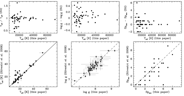
Figure 9: Comparison of the white dwarf effective temperatures and surface gravities and the spectral types of the secondary stars determined from our fits (Sect. 3.2, 3.3 and Table LABEL:t-pcebfit), and those of Silvestri et al. (2006). Top panels, from left to right: the WD effective temperature and surface gravity ratios, and the difference in the secondary’s spectral types from the two studies as a function of the white dwarf temperature.

Hence, combining the radial velocity information from Table 1 with the stellar parameters from Table LABEL:t-pcebfit, we determined upper limits to the orbital periods of all PCEBs and PCEB candidates, which range between 0.46–7880 d. The actual periods are likely to be substantially shorter, especially for those systems where only two SDSS spectra are available and the phase sampling is correspondingly poor. More stringent constraints could be obtained from a more complex exercise where the mid-exposure times are taken into account – however, given the fact that many of the SDSS spectra are combined from data taken on different nights, we refrained from this approach.

4.3 The fraction of PCEB among the SDSS WDMS binaries

We have measured the radial velocities of 101 WDMS which have multiple SDSS spectra, and find that 15 of them clearly show radial velocity variations, three additional WDMS are good candidates for radial velocity variations (see Table 1). Taking the upper limits to the orbital periods at face value, and assuming that systems with a period $\la 300$ d have undergone a CE (Willems & Kolb 2004, see also Sect. 2) 17 of the systems in Table 1 qualify as PCEBs, implying a PCEB fraction of $\sim$15 % in our WDMS sample, which is in rough agreement with the predictions by the population model of Willems & Kolb (2004). However, our value is likely to be a lower limit on the true fraction of PCEBs among the SDSS WDMS binares for the following reasons. (1) In most cases only two spectra are available, with a non-negligible chance of sampling similar orbital phases in both observations. (2) The relatively low spectral resolution of the SDSS spectroscopy ($\lambda/\Delta\lambda\simeq 1800$) plus the uncertainty in the flux calibration limit the detection of significant radial velocity changes to $\sim 15\,\mathrm{km\,s^{-1}}$ for the best spectra. (3) In binaries with extremely short orbital periods the long exposures will smear the Na I doublet beyond recognition. (4) A substantial number of the SDSS spectra are combined, averaging different orbital phases and reducing the sensitivity to radial velocity changes. Follow-up observations of a representative sample of SDSS WDMS with higher spectral resolution and a better defined cadence will be necessary for an accurate determination of the fraction of PCEBs.

4.4 Comparison with Raymond et al. (2003)

In a previous study, Raymond et al. (2003) determined white dwarf temperatures, distance estimates based on the white dwarf fits, and spectral types of the companion star for 109 SDSS WDMS. They restricted their white dwarf fits to a single gravity, $\log g=8.0$, and a white dwarf radius of $8\times 10^{8}$ cm (corresponding to $M_{\mathrm{wd}}=0.6$ M_⊙), which is a fair match for the majority of systems (see Sect. 4.6 below). Our sample of WDMS with two or more SDSS spectra has 28 objects in common with Raymond’s list, sufficient to allow for a quantitative comparison between the two different methods used to fit the data. As we fitted two or more spectra for each WDMS, we averaged for this purpose the parameters obtained from the fits to individual spectra of a given object, and propagated their errors accordingly. We find that $\sim 2/3$ of the temperatures determined by Raymond et al. (2003) agree with ours at the $\sim 20$ per cent level, with the remaining being different by up to a factor two (Fig. 8, left panels). This fairly large disagreement is most likely caused by the simplified fitting Raymond et al. adopted, i.e. fitting the white dwarf models in the wavelength range 3800–5000 Å, neglecting the contribution of the companion star. The spectral types of the companion stars from our work and Raymond et al. (2003) agree mostly to within $\pm 1.5$ spectral classes, which is satisfying given the composite nature of the WDMS spectra and the problems associated with their spectral decomposition (Fig. 8, right panels). The biggest discrepancy shows up in the distances, with the Raymond et al. distances being systematically lower than ours (Fig. 8, middle panels). The average of the factor by which Raymond et al. underpredict the distances is 6.5, which is close to $2\pi$, suggesting that the authors may have misinterpreted the flux definition of the model atmosphere code they used (TLUSTY/SYNSPEC from Hubeny & Lanz 1995, which outputs Eddington fluxes), and hence may have used a wrong constant in the flux normalisation (Eq. 3).

4.5 Comparison with Silvestri et al. (2006)

Having developed an independent method of determining the stellar parameters for WDMS from their SDSS spectra, we compared our results to those of Silvestri et al. (2006). As in Sect. 4.4 above, we average the parameters obtained from the fits to the individual SDSS spectra of a given object. Figure 9 shows the comparison between the white dwarf effective temperatures, surface gravities, and spectral types of the secondary stars from the two studies. Both studies agree in broad terms for all three fit parameters (Fig. 9, bottom panels). Inspecting the discrepancies between the two independent sets of stellar parameters, it became evident that relatively large disagreements are most noticeably found for $\mbox{$T_{\mathrm{eff}}$}\la 20\,000$ K, with differences in $T_{\mathrm{eff}}$ of up to a factor two, an order of magnitude in surface gravity, and a typical difference in spectral type of the secondary of $\pm 2$ spectral classes. For higher temperatures the differences become small, with nearly identical values for $T_{\mathrm{eff}}$, $\log g$ agreeing within $\pm 0.2$ magnitude, and spectral types differing by $\pm 1$ spectral classes at most (Fig. 9, top panels). We interpret this strong disagreement at low to intermediate white dwarf temperatures to the ambiguity between hot and cold solutions described in Sect. 3.3.

A quantitative judgement of the fits in Silvestri et al. (2006) is difficult, as the authors do not provide much detail on the method used to decompose the WDMS spectra, except for a single example in their Fig. 1. It is worth noting that the M dwarf component in that figure displays constant flux at $\lambda<6000$ Å, which seems rather unrealistic for the claimed spectral type of M5. Unfortunately, Silvestri et al. (2006) do not list distances implied by their fits to the white dwarf and main sequence components in their WDMS sample, which would provide a test of internal consistency (see Sect. 4.7).

We also investigated the systems Silvestri et al.’s (2006) method failed to fit, and found that we were able to determine reasonable parameters for the majority of them. It appears that our method is more robust in cases of low signal-to-noise ratio, and in cases where one of the stellar components contributes relatively little to the total flux. Examples of the latter are SDSS J204431.45–061440.2, where an M0 secondary star dominates the SDSS spectrum at $\lambda\ga 4600$ Å, or SDSS J172406.14+562003.1, which is a close PCEB containing a hot white dwarf and a low-mass companion. An independent analysis of the entire WDMS sample from SDSS appears therefore a worthwhile exercise, which we will pursue elsewhere.

4.6 Distribution of the stellar parameters

Having determined stellar parameters for each individual system in Sect. 3, we are looking here at their global distribution within our sample of WDMS. Figure. 10 shows histograms of the white dwarf effective temperatures, masses, $\log g$, and the spectral types of the main-sequence companions.

As in Sect. 4.4 and 4.5 above, we use here the average of the fit parameters obtained from the different SDSS spectra of each object. Furthermore, we exclude all systems with relative errors in their white dwarf parameters ($T_{\mathrm{wd}},\log g,M_{\mathrm{wd}}$) exceeding 25 per cent to prevent smearing of the histograms due to poor quality data and/or fits, which results in 95, 81, 94, and 38 WDMS in the histograms for the companion spectral type, $\log g$, $T_{\mathrm{wd}}$, and $M_{\mathrm{wd}}$, respectively. In broad terms, our results are consistent with those of Raymond et al. (2003) and Silvestri et al. (2006): the most frequent white dwarf temperatures are between 10 000–20 000 K, white dwarf masses cluster around $M_{\mathrm{wd}}\simeq 0.6$ M_⊙, and the companion stars have most typically a spectral type M3–4, with spectral types later than M7 or earlier than M1 being very rare.

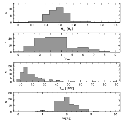
Figure 10: White dwarf mass, Sp types of the secondaries, effective temperature and $\log g$ histograms obtained from the SDSS WDSS sample. Excluded are those systems with individual WD masses, $T_{\mathrm{eff}}$, and $\log g$ associated to relative errors larger than 25 per cent.

At closer inspection, the distribution of white dwarf masses in our sample has a more pronounced tail towards lower masses compared to the distribution in Silvestri et al. (2006). A tail of lower-mass white dwarfs, peaking around 0.4 M_⊙ is observed also in well-studied samples of single white dwarfs (e.g. Liebert et al., 2005), and is interpreted as He-core white dwarfs descending from evolution in a binary star (e.g. Marsh et al., 1995). In a sample of WDMS, a significant fraction of systems will have undergone a CE phase, and hence the fraction of He-core white dwarfs among WDMS is expected to be larger than in a sample of single white dwarfs.

Also worth noting is that our distribution of companion star spectral types is relatively flat between M2–M4, more similar to the distribution of single M-dwarfs in SDSS (West et al., 2004) than the companion stars in Silvestri et al. (2006). More generally speaking, the cut-off at early spectral types is due to the fact that WDMS with K-type companions can only be identified from their spectra/colours if the white dwarf is very hot – and hence, very young, and correspondingly only few of such systems are in the total SDSS WDMS sample. The cut-off seen for low-mass companions is not so trivial to interpret. Obviously, very late-type stars are dim and will be harder to be detected against a moderately hot white dwarf, such a bias was discussed by Schreiber & Gänsicke (2003) for a sample of $\sim 30$ well-studied WDMS which predominantly originated from blue-colour ( = hot white dwarf) surveys. However, old WDMS with cool white dwarfs should be much more common (Schreiber & Gänsicke, 2003), and SDSS, sampling a much broader colour space than previous surveys, should be able to identify WDMS containing cool white dwarfs plus very late type companions. The relatively low frequency of such systems in the SDSS spectroscopic data base suggests that either SDSS is not efficiently targeting those systems for spectroscopic follow-up, or that they are rare in the first place, or a combination of both. A detailed discussion is beyond the scope of this paper, but we note that Farihi et al. (2005) have constructed the relative distribution of spectral types in the local M/L dwarf distribution, which peaks around M3–4, and steeply declines towards later spectral types, suggesting that late-type companions to white dwarfs are intrinsically rare. This is supported independently by Grether & Lineweaver (2006), who analysed the mass function of companions to solar-like stars, and found that it steeply decreases towards the late end of the main sequence (but rises again for planet-mass companions, resulting in the term ”brown dwarf desert”).

An assessment of the stellar parameters of all WDMS in SDSS DR5 using our spectral decomposition and white dwarf fitting method will improve the statistics of the distributions presented here, and will be presented in a future paper.

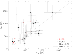
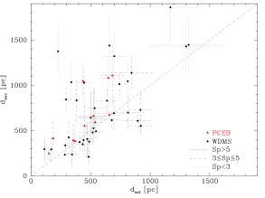
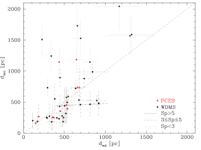
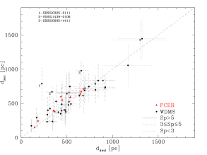
Figure 11: Comparison of $d_{\mathrm{sec}}$ and $d_{\mathrm{wd}}$ obtained from our spectral decomposition and white dwarf fits to the SDSS spectra. Approximately a third of the systems have $d_{\mathrm{sec}}\neq d_{\mathrm{wd}}$. The left panel splits the sample according to the mass of the white dwarfs, while the right panel divides the sample according to the spectral types of the secondaries. In both panels systems that we identify as PCEBs from radial velocity variations in their SDSS spectra are shown in red.

Figure 12: Left panel: the distances implied by the spectral decomposition were calculated by using the $Sp-R$ relation predicted by the models of Baraffe et al. (1998), instead of our empirical $Sp-R$ relation. Right panel: the spectral types of the secondary stars were adjusted by 1–2 spectral classes to achieve $d_{\mathrm{wd}}=d_{\mathrm{sec}}$. Only three systems can not be reconciled in this way, and are discussed individually in the text. We suggest that stellar activity in some WDMS may change the spectral type of their secondary stars, being equivalent to a change in surface temperature by a few 100 K.

4.7 Stellar activity on the secondary stars?

As outlined in Sect. 3.5, the scaling factors used in the modelling of the two spectral components of each WDMS provide two independent estimates of the distance to the system. In principle, both estimates should agree within their errors. Figure 12 compares the white dwarf and secondary star distance estimates obtained in Sect. 3.5, where the distances obtained from the individual SDSS spectra of a given object were averaged, and the errors accordingly propagated. In this plot, we exclude systems with relative errors in $d_{\mathrm{wd}}$ larger than 25 per cent to avoid cluttering by poor S/N data. The relative error in $d_{\mathrm{sec}}$ is dominated by the scatter in the $Sp-R$ relation, which represents an intrinsic uncertainty rather than a statistical error in the fit, and we therefore did not apply any cut in $d_{\mathrm{sec}}$. Taking the distribution of distances at face value, it appears that about $2/3$ of the systems have $d_{\mathrm{sec}}\simeq d_{\mathrm{wd}}$ within their 1$\sigma$ errors, as expected from purely statistical errors. However, there is a clear trend for outliers where $d_{\mathrm{sec}}>d_{\mathrm{wd}}$. We will discuss the possible causes and implications in the following sections.

4.7.1 Possible causes for $d_{\mathrm{sec}}\neq d_{\mathrm{wd}}$

We identify a number of possible causes for the discrepancy between the two independent distance estimates observed in $\sim 1/3$ of the WDMS analysed here.

(1) A tendency for systematic problems in the white dwarf fits? $d_{\mathrm{sec}}>d_{\mathrm{wd}}$ could be a result of too small white dwarf radii for a number of systems, i.e. too high white dwarf masses. We therefore identify in the left panel of Fig. 12 those systems with massive $(>0.75$ M${}_{\odot})$ white dwarfs. It is apparent that the outliers from the $d_{\mathrm{sec}}=d_{\mathrm{wd}}$ relation do not contain a large number of very massive white dwarfs.

(2) Problems in determining the correct spectral type of the secondary? If the error on the spectral type of the companion star determined from the spectral decomposition is larger than $\pm 0.5$, as assumed in Sect. 3.2, a substantial deviation from $d_{\mathrm{sec}}=d_{\mathrm{wd}}$ would result. However, as long as this error is symmetric around the true spectral type, it would cause scatter on both sides of the $d_{\mathrm{sec}}=d_{\mathrm{wd}}$ relation. Only if the determined spectral types were consistently too early for $\sim 1/3$ of the systems, the observed preference for outliers at $d_{\mathrm{sec}}>d_{\mathrm{wd}}$ could be explained (see Sect. 4.7.2 below for a hypothetical systematic reason for spectral types that are consistently too early).

(3) Problems in the spectral type-radius relation? As discussed in Sect. 3.4, the spectral type-radius relation of late type stars is not particularly well defined. The large scatter of observed radii at a given spectral type is taken into account in the errors in $d_{\mathrm{sec}}$. If those errors were underestimated, they should cause an approximatively symmetric scatter of systems around $d_{\mathrm{sec}}=d_{\mathrm{wd}}$, which is not observed (the $Sp-R$ relation being non-linear lead to asymmetric error bars in the radius for a given symmetric error in the spectral type, however, over a reasonably small range in the spectral type this effect is negligible). A systematic problem over a small range of spectral types would result in a concentration of the affected spectral types among the outliers. For this purpose, we divide our sample into three groups of secondary star spectral classes, Sp $>$ 5, 3 $\leq$ Sp $\leq$ 5, and Sp $<$ 3 (Fig. 12, right panel). The outliers show a slight concentration towards early types (Sp $<$ 3) compared to the distribution of secondary star spectral types in the total sample (Fig.  10).

To explore the idea that our empirical $Sp-R$ relation is simply inadequate, we calculated a new set of secondary star distances, using the theoretical $Sp-R$ relation from Baraffe et al. (1998) (see Fig. 7, bottom panel), which are shown in the left panel of Fig. 12. The theoretical $Sp-R$ relation implies smaller radii in the range M3–M6, but the difference with our empirical relation is not sufficient enough to shift the outlying WDMS onto the $d_{\mathrm{sec}}=d_{\mathrm{wd}}$ relation. For spectral types earlier than M2.5, our empirical $Sp-R$ relation actually gives smaller radii than the theoretical Baraffe et al. 1998 relation, so that using the theoretical $Sp-R$ actually exacerbates the $d_{\mathrm{sec}}>d_{\mathrm{wd}}$ problem.

(4) A relationship with close binarity? The fraction of PCEBs among the outliers is similar to the fraction among the total sample of WDMS (Fig. 12), hence it does not appear that close binarity is a decisive issue.

(5) An age effect? Late type stars take a long time to contract to their zero age main sequence (ZAMS) radii, and if some of the WDMS in our sample were relatively young objects, their M-dwarfs would tend to have larger radii than ZAMS radii. As briefly discussed in Footnote 4, the majority of the WDMS in our sample are likely to be older than $\sim 1$ Gyr, and the outliers in Fig.  12,12 do not show any preference for hot or massive white dwarfs, which would imply short cooling ages and main sequence life times.

4.7.2 Could stellar activity affect Sp_sec?

None of the points discussed in the previous section conclusively explains the preference for outliers having $d_{\mathrm{sec}}>d_{\mathrm{wd}}$. If we assume that the problem rests in the determined properties of the secondary star, rather than those of the white dwarf, the immediate implication of $d_{\mathrm{sec}}>d_{\mathrm{wd}}$ is that the assumed radii of the secondary stars are too large. As mentioned above and shown in Fig.  12, this statement does not strongly depend on which $Sp-R$ relation we use to determine the radii, either our empirical relation or the theoretical Baraffe et al. (1998) relation. Rather than blaming the radii, we explore here whether the secondary star spectral types determined from our decomposition of the SDSS spectra might be consistently too early in the outlying systems. If this was the case, we would pick a radius from our $Sp-R$ relation that is larger than the true radius of the secondary star, resulting in too large a distance. In other words, the question is: is there a mechanism that could cause the spectral type of an M-star, as derived from low-resolution optical spectroscopy, to appear too early?

The reaction of stars to stellar activity on their surface, also referred to as spottedness is a complex phenomenon that is not fully understood. Theoretical studies (e.g. Spruit & Weiss, 1986; Mullan & MacDonald, 2001; Chabrier et al., 2007) agree broadly on the following points: (1) the effect of stellar activity is relatively weak at the low-mass end of the main sequence ($M\la 0.3$ M_⊙), where stars are conventionally thought to become fully convective (though, see Mullan & MacDonald 2001; Chabrier et al. 2007 for discussions on how magnetic fields may change that mass boundary), (2) stellar activity will result in an increase in radius, and (3) the effective temperature of an active star is lower than that of an unspotted star.

Here, we briefly discuss the possible effects of stellar activity on the spectral type of a star. For this purpose, it is important not to confuse the effective temperature, which is purely a definition coupled to the luminosity and the stellar radius via $L=4\pi R^{2}\sigma T_{\mathrm{eff}}^{4}$ (and hence is a global property of the star), and the local temperature of a given part of the stellar surface, which will vary from spotted areas to inter-spot areas. In an unspotted star effective and local temperature are the same, and both colour and spectral type are well-defined. As a simple example to illustrate the difference between effective temperature and colour in an active star, we assume that a large fraction of the star is covered by zero-temperature, i.e. black spots, and that the inter-spot temperature is the same as that of the unspotted star. As shown by Chabrier et al. (2007), assuming constant luminosity requires the radius of the star to increase, and the effective temperature to drop. Thus, while intuition would suggest that a lower effective temperature would result in a redder colour, this ficticious star has exactly the same colour and spectral type as its unspotted equivalent – as the black spots contribute no flux at all, and the inter-spot regions with the same spectral shape as the unspotted star.

Obviously, the situation in a real star will be more complicated, as the spots will not be black, but have a finite temperature, and the star will hence have a complicated temperature distribution over its surface. Thus, the spectral energy distribution of such a spotted star will be the superposition of contributions of different temperatures, weighted by their respective covering fraction of the stellar surface. Strictly speaking, such a star has no longer a well-defined spectral type or colour, as these properties will depend on the wavelength range that is observed. Spruit & Weiss (1986) assessed the effect of long-term spottedness on the temperature distribution on active stars, and found that for stars with masses in the range $0.3-0.6$ M_⊙ the long-term effect of spots is to increase the temperature of the inter-spot regions by $\sim 100-200$ K (compared to the effective temperature of the equivalent unspotted star), wheras the inter-spot temperature of spotted lower-mass stars remains unchanged. Spruit & Weiss (1986) also estimated the effects of stellar activity on the colours of stars, but given their use of simple blackbody spectra, these estimates are of limited value. As a general tendency, the hotter (unspotted) parts of the star will predominantly contribute in the blue end of the the spectral energy distribution, the cooler (spotted) ones in its red end. As we determine the spectral types of the secondary stars in the SDSS WDMS from optical ( = blue) spectra, and taking the results of Spruit & Weiss at face value, it appears hence possible that they are too early compared to unspotted stars of the same mass. A full theoretical treatment of this problem would involve calculating the detailed surface structure of active stars as well as appropriate spectral models for each surface element in order to compute the spatially integreated spectrum as it would be observed. This is clearly a challenging task.

Given that theoretical models on the effect of stellar activity have not yet converged, and are far from making detailed predictions on the spectroscopic appearence of active stars, we pursue here an empirical approach. We assume that the discrepancy $d_{\mathrm{sec}}>d_{\mathrm{wd}}$ results from picking a spectral type too early, i.e. we assume that the secondary star appears hotter in the optical spectrum that it should for its given mass. Then, we check by how much we have to adjust the spectral type (and the corresponding radius) to achieve $d_{\mathrm{sec}}=d_{\mathrm{wd}}$ within the errors. We find that the majority of systems need a change of 1–2 spectral classes, which corresponds to changes in the effective temperature of a few hundred degrees only, in line with the calculations of Spruit & Weiss (1986). Bearing in mind that what we see in the optical is the surface temperature, and not the effective temperature, comparing this to the surface temperature changes calculated by Spruit & Weiss (1986), and taking into account that we ignored in this simple approach the change in radius caused by a large spottedness, it appears plausible that the large deviations from $d_{\mathrm{sec}}=d_{\mathrm{wd}}$ may be related to stellar activity on the secondary stars.

There are three WDMS where a change of more than two spectral classes would be necessary: SDSSJ032510.84-011114.1, SDSSJ093506.92+441107.0, and SDSSJ143947.62-010606.9. SDSSJ143947.62-010606.9 contains a very hot white dwarf, and the secondary star may be heated if this system is a PCEB. Its two SDSS spectra reveal no significant radial velocity variation, but as discussed in Sect. 2 the SDSS spectra can not exclude a PCEB nature because of random phase sampling, low inclination and limited spectral resolution. SDSSJ032510.84-011114.1 and SDSSJ093506.92+441107.0 could be short-period PCEBs, as they both have poorly define Na I absorption doublets, possibly smeared by orbital motion over the SDSS exposure (see Sect. 2). In a close binary, their moderate white dwarf temperatures would be sufficient to cause noticeable heating of the secondary star. We conclude that our study suggests some anomalies in the properties of $\sim 1/3$ of the M-dwarf companions within the WDMS sample analysed here. This is in line with previous detailed studies reporting the anomalous behaviour of the main sequence companions in PCEBs and cataclysmic variables, e.g. O’Brien et al. (2001) or Naylor et al. (2005).

4.8 Selection effects among the SDSS WDMS.

Selection effects among the WDMS found by SDSS with respect to the spectral type of their main-sequence component can be deduced from the right panel of Fig. 12. No binaries with econdary spectral types later than M5 are found at distances larger than $\sim 500$ pc. Because of their intrinsic faintness, such late-type secondary stars can only be seen against relatively cool white dwarfs, and hence the large absolute magnitude of such WDMS limits their detection within the SDSS magnitude limit to a relatively short distance. Hot white dwarfs in SDSS can be detected to larger distances, and may have undetected late-type companions. There are also very few WDMS with secondary stars earlier than M3 within 500 pc. In those systems, the secondary star is so bright that it saturates the $z$, and possibly the $i$ band, disqualifying the systems for spectroscopic follow up by SDSS. While these selection effects may seem dishearting at first, it will be possible to quantitatively correct them based on predicted colours of WDMS binaries and the information available within the SDSS project regarding photometric properties and spectroscopic selection algorithms.

5 Conclusions

We have identified 18 PCEBs and PCEB candidates among a sample of 101 WDMS for which repeat SDSS spectroscopic observations are available in DR5. From the SDSS spectra, we determine the spectral types of the main sequence companions, the effective temperatures, surface gravities, and masses of the white dwarfs, as well as distance estimates to the systems based both on the properties of the white dwarfs and of the main sequence stars. In about 1/3 of the WDMS studied here the SDSS spectra suggest that the secondary stars have either radii that are substantially larger than those of single M-dwarfs, or spectral types that are too early for their masses. Follow-up observations of the PCEBs and PCEB candidates is encouraged in order to determine their orbital periods as well as more detailed system parameters. Given the fact that we have analysed here only $\sim 10$ per cent of the WDMS in DR5, it is clear SDSS holds the potential to dramatically improve our understanding of CE evolution.

Table 5: WD masses, effective temperatures, surface gravities, spectral types and distances of the SDSS PCEBs identified in Sect. 3, as determined from spectral modelling. The stellar parameters for the remaining 112 WDMS binaries can be found in the electronic edition of the paper. We quote by and $s$ and $e$ those systems which have been studied previously by Silvestri et al. (2006) and Eisenstein et al. (2006), repectively.

SDSS J	MJD	plate	fiber	$T_{\mathrm{eff}}$(K)	err	$\log g$	err	$M(M_{\bigodot})$	err	$d_{\mathrm{wd}}$(pc)	err	Sp	$d_{\mathrm{sec}}$(pc)	err	flag	notes
005245.11-005337.2	51812	394	96	15071	4224	8.69	0.73	1.04	0.38	505	297	4	502	149	s,e
	51876	394	100	17505	7726	9.48	0.95	1.45	0.49	202	15	4	511	152
	51913	394	100	16910	2562	9.30	0.42	1.35	0.22	261	173	4	496	147
	52201	692	211	17106	3034	9.36	0.43	1.38	0.22	238	178	4	526	156
005457.61-002517.0	51812	394	118	16717	574	7.81	0.13	0.51	0.07	455	38	5	539	271	s,e
	51876	394	109	17106	588	7.80	0.14	0.51	0.07	474	40	5	562	283
	51913	394	110	17106	290	7.88	0.07	0.55	0.04	420	19	5	550	277
022503.02+005456.2	51817	406	533	-	-	-	-	-	-	-	-	5	341	172	s,e	1
	51869	406	531	-	-	-	-	-	-	-	-	5	351	177
	51876	406	532	-	-	-	-	-	-	-	-	5	349	176
	51900	406	532	-	-	-	-	-	-	-	-	5	342	172
	52238	406	533	-	-	-	-	-	-	-	-	5	356	179
024642.55+004137.2	51871	409	425	15782	5260	9.18	0.76	1.29	0.39	213	212	4	365	108	s,e
	52177	707	460	-	-	-	-	-	-	-	-	3	483	77
	52965	1664	420	16717	1434	8.45	0.28	0.90	0.16	515	108	3	492	78
	52973	1664	407	14065	1416	8.24	0.22	0.76	0.14	510	77	3	499	80
025147.85-000003.2	52175	708	228	17106	4720	7.75	0.92	0.49	0.54	1660	812	4	881	262	e	2
	52177	707	637	-	-	-	-	-	-	-	-	4	794	236
030904.82-010100.8	51931	412	210	19416	3324	8.18	0.68	0.73	0.40	1107	471	3	888	141	s,e
	52203	710	214	18756	5558	9.07	0.61	1.24	0.31	462	325	3	830	132
	52235	412	215	14899	9359	8.94	1.45	1.17	0.75	374	208	4	586	174
	52250	412	215	11173	9148	8.55	1.60	0.95	0.84	398	341	4	569	169
	52254	412	201	20566	7862	8.82	0.72	1.11	0.37	627	407	3	836	133
	52258	412	215	19640	2587	8.70	0.53	1.04	0.27	650	281	3	854	136
	53386	2068	126	15246	4434	8.75	0.79	1.07	0.41	522	348	4	628	187
031404.98-011136.6	51931	412	45	-	-	-	-	-	-	-	-	4	445	132	s,e	1
	52202	711	285	-	-	-	-	-	-	-	-	4	475	141
	52235	412	8	-	-	-	-	-	-	-	-	4	452	134
	52250	412	2	-	-	-	-	-	-	-	-	4	426	126
	52254	412	8	-	-	-	-	-	-	-	-	4	444	132
	52258	412	54	-	-	-	-	-	-	-	-	4	445	132
082022.02+431411.0	51959	547	76	21045	225	7.94	0.04	0.59	0.02	153	4	4	250	74	s,e
	52207	547	59	21045	147	7.95	0.03	0.60	0.01	147	2	4	244	72
113800.35-001144.4	51630	282	113	18756	1364	7.99	0.28	0.62	0.17	588	106	4	601	178	s,e
	51658	282	111	24726	1180	8.34	0.16	0.84	0.10	487	60	4	581	173
115156.94-000725.4	51662	284	435	10427	193	7.90	0.23	0.54	0.14	180	25	5	397	200	s,e
	51943	284	440	10189	115	7.99	0.16	0.59	0.10	191	19	5	431	217
152933.25+002031.2	51641	314	354	14228	575	7.67	0.12	0.44	0.05	338	25	5	394	199	s,e
	51989	363	350	14728	374	7.59	0.09	0.41	0.04	372	21	5	391	197
172406.14+562003.0	51813	357	579	35740	187	7.41	0.04	0.42	0.01	417	15	2	1075	222	s,e
	51818	358	318	36154	352	7.33	0.06	0.40	0.02	453	24	2	1029	213
	51997	367	564	37857	324	7.40	0.04	0.43	0.01	439	16	2	1031	213
172601.54+560527.0	51813	357	547	20331	1245	8.24	0.23	0.77	0.14	582	94	2	1090	225	s,e
	51997	367	548	20098	930	7.94	0.18	0.59	0.11	714	83	2	1069	221
173727.27+540352.2	51816	360	165	13127	1999	7.91	0.42	0.56	0.26	559	140	6	680	307	s,e
	51999	362	162	13904	1401	8.24	0.31	0.76	0.20	488	106	6	639	288
224139.02+002710.9	53261	1901	471	12681	495	8.05	0.15	0.64	0.09	369	35	4	381	113	e
	52201	674	625	13745	1644	7.66	0.36	0.43	0.19	524	108	4	378	112
233928.35-002040.0	53357	1903	264	15071	1858	8.69	0.33	1.04	0.18	416	112	4	530	157	e
	52525	682	159	12536	2530	7.92	0.79	0.56	0.48	655	291	4	528	157
234534.49-001453.7	52524	683	166	19193	1484	7.79	0.31	0.51	0.17	713	132	4	1058	314	s,e	5
	53357	1903	103	18974	730	7.98	0.15	0.61	0.09	652	62	4	1155	343
235020.76-002339.9	51788	386	228	-	-	-	-	-	-	-	-	5	504	254		6
	52523	684	226	-	-	-	-	-	-	-	-	5	438	22
(1) $T_{\mathrm{eff}}$  less than 6000; (2) Noisy spectra; (3) Cold WD; (4) Diffuse background galaxy in the SDSS image; (5) Reflection effect; (6) Some blue excess, WD?

References

- Adelman-McCarthy et al. (2006) Adelman-McCarthy, J. K., et al., 2006, ApJS, 162, 38
- Baraffe & Chabrier (1996) Baraffe, I., Chabrier, G., 1996, ApJ Lett., 461, L51
- Baraffe et al. (1998) Baraffe, I., Chabrier, G., Allard, F., Hauschildt, P. H., 1998, A&A, 337, 403
- Bayless & Orosz (2006) Bayless, A. J., Orosz, J. A., 2006, ApJ, 651, 1155
- Beatty et al. (2007) Beatty, T. G., et al., 2007, ArXiv e-prints, 704
- Berger et al. (2006) Berger, D. H., et al., 2006, ApJ, 644, 475
- Berger (2002) Berger, E., 2002, ApJ, 572, 503
- Bergeron et al. (1995) Bergeron, P., Wesemael, F., Beauchamp, A., 1995, PASP, 107, 1047
- Berriman & Reid (1987) Berriman, G., Reid, N., 1987, MNRAS, 227, 315
- Beuermann (2006) Beuermann, K., 2006, A&A, 460, 783
- Beuermann et al. (1998) Beuermann, K., Baraffe, I., Kolb, U., Weichhold, M., 1998, A&A, 339, 518
- Bochanski et al. (2007) Bochanski, J. J., West, A. A., Hawley, S. L., Covey, K. R., 2007, AJ, 133, 531
- Caillault & Patterson (1990) Caillault, J., Patterson, J., 1990, AJ, 100, 825
- Chabrier et al. (2007) Chabrier, G., Gallardo, J., Baraffe, I., 2007, A&A, in press, arXiv:0707.1792
- Creevey et al. (2005) Creevey, O. L., et al., 2005, ApJ Lett., 625, L127
- Cushing et al. (2005) Cushing, M. C., Rayner, J. T., Vacca, W. D., 2005, ApJ, 623, 1115
- De Marco et al. (2004) De Marco, O., Bond, H. E., Harmer, D., Fleming, A. J., 2004, ApJ Lett., 602, L93
- Delfosse et al. (1998) Delfosse, X., Forveille, T., Perrier, C., Mayor, M., 1998, A&A, 331, 581
- Delfosse et al. (1999) Delfosse, X., Forveille, T., Mayor, M., Burnet, M., Perrier, C., 1999, A&A, 341, L63
- Dobbie et al. (2006) Dobbie, P. D., et al., 2006, MNRAS, 369, 383
- Eisenstein et al. (2006) Eisenstein, D. J., et al., 2006, ApJS, 167, 40
- Farihi et al. (2005) Farihi, J., Becklin, E. E., Zuckerman, B., 2005, ApJS, 161, 394
- Golimowski et al. (2004) Golimowski, D. A., et al., 2004, AJ, 127, 3516
- Grether & Lineweaver (2006) Grether, D., Lineweaver, C. H., 2006, ApJ, 640, 1051
- Haefner et al. (2004) Haefner, R., Fiedler, A., Butler, K., Barwig, H., 2004, A&A, 428, 181
- Hubeny & Lanz (1995) Hubeny, I., Lanz, T., 1995, ApJ, 439, 875
- Iben (1991) Iben, I. J., 1991, ApJS, 76, 55
- Iben & Livio (1993) Iben, I. J., Livio, M., 1993, PASP, 105, 1373
- Kepler et al. (2006) Kepler, S. O., Castanheira, B. G., Costa, A. F. M., Koester, D., 2006, MNRAS, 372, 1799
- Koester et al. (2005) Koester, D., Napiwotzki, R., Voss, B., Homeier, D., Reimers, D., 2005, A&A, 439, 317
- Lane et al. (2001) Lane, B. F., Boden, A. F., Kulkarni, S. R., 2001, ApJ Lett., 551, L81
- Leggett et al. (1996) Leggett, S. K., Allard, F., Berriman, G., Dahn, C. C., Hauschildt, P. H., 1996, ApJS, 104, 117
- Leggett et al. (2001) Leggett, S. K., Allard, F., Geballe, T. R., Hauschildt, P. H., Schweitzer, A., 2001, ApJ, 548, 908
- Leto et al. (2000) Leto, G., Pagano, I., Linsky, J. L., Rodonò, M., Umana, G., 2000, A&A, 359, 1035
- Liebert et al. (2005) Liebert, J., Bergeron, P., Holberg, J. B., 2005, ApJS, 156, 47
- Livio & Soker (1988) Livio, M., Soker, N., 1988, ApJ, 329, 764
- López-Morales (2007) López-Morales, M., 2007, ApJ, 660, 732
- Maceroni & Montalbán (2004) Maceroni, C., Montalbán, J., 2004, A&A, 426, 577
- Marsh & Duck (1996) Marsh, T. R., Duck, S. R., 1996, MNRAS, 278, 565
- Marsh et al. (1995) Marsh, T. R., Dhillon, V. S., Duck, S. R., 1995, MNRAS, 275, 828
- Mateo et al. (1985) Mateo, M., Szkody, P., Bolte, M., 1985, PASP, 97, 45
- Maxted et al. (2004) Maxted, P. F. L., Marsh, T. R., Morales-Rueda, L., Barstow, M. A., Dobbie, P. D., Schreiber, M. R., Dhillon, V. S., Brinkworth, C. S., 2004, MNRAS, 355, 1143
- Maxted et al. (2006) Maxted, P. F. L., Napiwotzki, R., Dobbie, P. D., Burleigh, M. R., 2006, Nat, 442, 543
- Maxted et al. (2007) Maxted, P. F. L., O’Donoghue, D., Morales-Rueda, L., Napiwotzki, R., 2007, MNRAS, 376, 919
- Montagnier et al. (2006) Montagnier, G., et al., 2006, A&A, 460, L19
- Mullan & MacDonald (2001) Mullan, D. J., MacDonald, J., 2001, ApJ, 559, 353
- Naylor et al. (2005) Naylor, T., Allan, A., Long, K. S., 2005, MNRAS, 361, 1091
- Nelemans & Tout (2005) Nelemans, G., Tout, C. A., 2005, MNRAS, 356, 753
- Nelemans et al. (2000) Nelemans, G., Verbunt, F., Yungelson, L. R., Portegies Zwart, S. F., 2000, A&A, 360, 1011
- O’Brien et al. (2001) O’Brien, M. S., Bond, H. E., Sion, E. M., 2001, ApJ, 563, 971
- O’Donoghue et al. (2003) O’Donoghue, D., Koen, C., Kilkenny, D., Stobie, R. S., Koester, D., Bessell, M. S., Hambly, N., MacGillivray, H., 2003, MNRAS, 345, 506
- Paczynski (1976) Paczynski, B., 1976, in Eggleton, P., Mitton, S., Whelan, J., eds., IAU Symp. 73: Structure and Evolution of Close Binary Systems, D. Reidel, Dordrecht, p. 75
- Pont et al. (2005) Pont, F., Melo, C. H. F., Bouchy, F., Udry, S., Queloz, D., Mayor, M., Santos, N. C., 2005, A&A, 433, L21
- Raymond et al. (2003) Raymond, S. N., et al., 2003, AJ, 125, 2621
- Rechenberg (1994) Rechenberg, I., 1994, Evolutionsstrategie ’94, Froomann–Holzboog, Stuttgart
- Ribas (2006) Ribas, I., 2006, ASS, 304, 89
- Schreiber et al. (2007) Schreiber, M., Nebot Gomez-Moran, A., Schwope, A., 2007, in Napiwotzki, R., Burleigh, R., eds., 15th European Workshop on White Dwarfs, ASP Conf. Ser., p. in press, astroph/0611461
- Schreiber & Gänsicke (2003) Schreiber, M. R., Gänsicke, B. T., 2003, A&A, 406, 305
- Ségransan et al. (2003) Ségransan, D., Kervella, P., Forveille, T., Queloz, D., 2003, A&A, 397, L5
- Silvestri et al. (2006) Silvestri, N. M., et al., 2006, AJ, 131, 1674
- Southworth et al. (2007) Southworth, J., Gänsicke, B., Schreiber, M., 2007, MNRAS, submitted
- Spruit & Weiss (1986) Spruit, H. C., Weiss, A., 1986, A&A, 166, 167
- Stoughton et al. (2002) Stoughton, C., et al., 2002, AJ, 123, 485
- Strauss et al. (2002) Strauss, M. A., et al., 2002, AJ, 124, 1810
- van den Besselaar et al. (2007) van den Besselaar, E. J. M., et al., 2007, A&A, 466, 1031
- Vogel et al. (2007) Vogel, J., Schwope, A. D., Gänsicke, B. T., 2007, A&A, 464, 647
- West et al. (2004) West, A. A., et al., 2004, AJ, 128, 426
- Willems & Kolb (2004) Willems, B., Kolb, U., 2004, A&A, 419, 1057
- York et al. (2000) York, D. G., et al., 2000, AJ, 120, 1579