Semiclassical theory of charged pion radiation by nucleons in a strong homogeneous magnetic field

Abstract

Charged pions produced in very high energy hadronic interactions might be the dominant source of cosmic neutrinos in the GeV–TeV range. Spectral energy power of $\pi^{+}$ radiation by high energy protons moving in strong magnetic fields typical for magnetars is determined with a semiclassical treatment of the effective pion-nucleon model. The main characteristics emerging from a saddle point approximation to the summation over the allowed range of Landau levels is a sharp lower cut: $E_{\pi}\geq 0.25E_{p}$. The magnitude of the spectral power agrees in this region with the synchrotron radiation spectra of neutral pions.

1 Charged pions as cosmic sources of high energy neutrinos

Identification of the cosmic sources of (ultra)high energy neutrinos will make a big leap forward with the completion of the construction of ICECUBE[1], KM3NeT[2] and other observatories specifically designed for neutrino observations, and also with the cosmic ray observatory P. Auger and its northern counterpart. At present theoretical arguments are put forward for neutrino production in gamma ray bursts[3], magnetars [4, 5], blazars[6], pulsars[7] and compact binary objects[8]. In general objects where protons might be accelerated to high enough energy to reach the threshold of pion production in various elementary reactions are worth to be investigated. High energy neutrinos are expected to arise from pion and subsequent muon decays.

The typical reaction chain in presence of hard enough $\gamma$ quanta is[9]

$$p+\gamma\rightarrow\Delta^{+}\rightarrow n+\pi^{+}\rightarrow n+\mu^{+}+\nu_{\mu}\rightarrow n+\nu_{\mu}+\nu_{e}+e^{+}+\bar{\nu}_{\mu}.$$ (1)

Energetic $\gamma$ quanta might arise from synchrotron radiation of fast protons moving on circular orbit in strong magnetic field of magnetars, for instance. In the estimation of the neutrino luminosity possible effects on proton acceleration arising from the presence of strong magnetic field were taken into account. Another mechanism proposed for $\pi^{+}$ production involves high energy proton-neutron collisions, assuming that also the latter component is present in the environment of a gamma ray burst[3]

$$p+n\rightarrow n+n+\pi^{+}\rightarrow 2n+\mu^{+}+\nu_{\mu}\rightarrow 2n+e^{+}+\nu_{e}+\bar{\nu}_{\mu}+\nu_{\mu}.$$ (2)

The problem of neutral pion production as a result of synchrotron radiation of pion field strongly coupled to the protons in presence of strong magnetic field $B$:

$$p+B\rightarrow p+\pi^{0}+B$$ (3)

was investigated first forty years ago by Ginzburg and Zharkov [10] and reviewed by Ginzburg and Sirovatski[11]. The treatment followed closely the classical theory of synchrotron radiation. It was shown to reproduce the results of first order quantum perturbation theory applied to an effective nucleon-pion interaction Hamiltonian. A perturbative estimate for the $p\rightarrow n+\pi^{+}$ transition probability under the influence of a strong electromagnetic wave (i.e. charged particles considered as Volkov states) was given at the same time by Zharkov[12].

At present much higher cosmic magnetic fields are known, in particular in magnetars, where $B=10^{14-16}$G was observed[13]. Substantial progress has been achieved also in the understanding of acceleration mechanisms. Therefore it is timely to evaluate the old formulae with the actual parameters. This task was partially done by Tokuhisa and Kajino[14], but no reassessment was attempted to date for the case of charged pions.

The subject of this note is to present a semiclassical theory for charged pion radiation in strong magnetic field:

$$p+B\rightarrow n+\pi^{+}+B$$ (4)

and estimate the luminosity of this radiation for the highest possible energy range. Since any individual proton contributes only a single positively charged pion into the radiation, it is hard to associate a classical charged pion source with a single proton. If one assumes a very intense proton beam, however, then the loss of a restricted number of protons should not mean a strong back reaction, e.g. the source remains approximately intact. This kind of approximation represents the main hypothesis of this work, which assumes unchanged proton source during the building up of a classical $\pi^{+}$ radiation field around the source.

2 The model

The Lagrangian of charged pions coupled to a nuclear source density is the following:

$$\mathcal{L}=(\partial_{\mu}-\mathrm{i}\,eA_{\mu})\pi^{+}(\partial_{\mu}+\mathrm{i}\,eA_{\mu})\pi^{-}-m^{2}\pi^{+}\pi^{-}-g\sqrt{2}(\rho_{N}^{-}\pi^{+}+\rho_{N}^{+}\pi^{-})\,,$$ (5)

where the nuclear source terms are $\rho_{N}^{-}=\mathrm{i}\,\bar{p}\gamma_{5}n$, $\rho_{N}^{+}=\mathrm{i}\,\bar{n}\gamma_{5}p$, and $g^{2}\approx 14.6$. (Throughout this paper the unit system $\hbar=c=1$ is used, SI values for some important dimensional combinations will be explicitly given below). The Euler–Lagrange equations of the pion fields, in Coulomb gauge ($A_{0}=0,\,\partial_{i}A_{i}=0$) read as

$$\left[\partial_{t}^{2}-\partial_{i}\partial_{i}\pm 2\,\mathrm{i}\,eA_{i}\partial_{i}+e^{2}A_{i}A_{i}+m^{2}\right]\pi^{\pm}=-g\sqrt{2}\rho^{\pm}_{N}\,.$$ (6)

In presence of a static magnetic field along the ’$z$’ direction ($\mathbf{B}=(0,0,B)$), it is useful to introduce cylindrical coordinates. Then (6) takes the following form:

$$\left[\partial_{t}^{2}-\frac{1}{\rho}\frac{\mathrm{d}}{\mathrm{d}\rho}\left(\rho\frac{\mathrm{d}}{\mathrm{d}\rho}\right)+\frac{1}{\rho^{2}}\frac{\mathrm{d^{2}}}{\mathrm{d}\phi^{2}}+\frac{\mathrm{d^{2}}}{\mathrm{d}z^{2}}\pm\mathrm{i}\,eB\frac{\partial}{\partial\phi}+\frac{1}{4}e^{2}B^{2}\rho^{2}+m^{2}\right]\pi^{\pm}=-g\sqrt{2}\rho^{\pm}_{N}\,.$$ (7)

The particular retarded solution describing the radiation of charged pions for the above linear partial differential equations is constructed as

$$\pi^{\pm}(\rho,\phi,z,t)=-g\sqrt{2}\int\mathrm{d}\rho^{\prime}\mathrm{d}\phi^{\prime}\mathrm{d}z^{\prime}\mathrm{d}t^{\prime}G^{\pm}(\rho,\phi,z,t;\rho^{\prime},\phi^{\prime},z^{\prime},t^{\prime})\rho_{N}^{\pm}(\rho^{\prime}\phi^{\prime},z^{\prime},t^{\prime}),$$ (8)

where the Green’s functions $G^{\pm}$ are determined by the eigenvalues and eigenfunctions of the differential operator of the left hand side of (7),

$$G^{+}(\rho,\phi,z,t;\rho^{\prime},\phi^{\prime},z^{\prime},t^{\prime})=\sum_{i}\frac{\Phi_{i}(\rho,\phi,z,t)\Phi_{i}^{\star}(\rho^{\prime},\phi^{\prime},z^{\prime},t^{\prime})}{\lambda_{i}}=(G^{-})^{\star}.$$ (9)

Writing the eigenfunctions in the form

$$\Phi=\mathrm{exp}\left[\mathrm{i}\,(\mu\phi+kz-\omega t)\right]R(x)\,,\qquad x=\frac{eB}{2}\rho^{2}\,,$$ (10)

the corresponding eigenvalue problem is reduced to the eigenvalue problem of an ordinary differential operator,

$$xR^{\prime\prime}+R^{\prime}-\left[\frac{x}{4}+\frac{\mu^{2}}{4x}-\frac{\mu}{2}-\frac{1}{2eB}\left(\omega^{2}-k^{2}-m^{2}\right)\right]R(x)=-\lambda R(x).$$ (11)

This is the well-known problem of the relativistic Landau-levels, with the normalized solution (see for example in [15] 22.6.16 and 22.2.12)

$$R_{n}^{\mu}(x)\!=\!\sqrt{\frac{\Gamma(n+1)}{\Gamma(n+|\mu|+1)}}\,\mathrm{e}^{-x/2}x^{|\mu|/2}L_{n}^{|\mu|}(x),\,\lambda=eB(2n+|\mu|-\mu+1)-\omega^{2}+k^{2}+m^{2},$$ (12)

where $L_{n}^{|\mu|}(x)$ denotes the generalized Laguerre polynomial, and $R_{n}^{\mu}(x)$ form a complete orthogonal set for $n=0,1,2,3,\ldots$ . The normalized eigenfunctions (10) are written in the following explicit form:

$$\Phi_{n,\mu,k,\omega}(\rho,\phi,z,t)=\sqrt{\frac{eB}{(2\pi)^{3}}}\,{\exp}\left[\mathrm{i}\,(\mu\phi+kz-\omega t)\right]R_{n}^{\mu}\left(\frac{eB}{2}\rho^{2}\right)$$ (13)

and the corresponding eigenvalues are listed in (12). From (9) the Green’s function is found after performing the $\omega$ integration:

$$G^{+}(\rho,\phi,z,t;\rho^{\prime},\phi^{\prime},z^{\prime},t^{\prime}) = \frac{eB}{(2\pi)^{2}}\int\mathrm{d}k\sum_{n=0}^{\infty}\sum_{\mu=-\infty}^{\infty}{\exp}\left[\mathrm{i}\,(\mu(\phi-\phi^{\prime})+k(z-z^{\prime}))\right]$$ (14)

$$\times R_{n}^{\mu}(\rho)R_{n}^{\mu}(\rho^{\prime})\frac{1}{A_{n,\mu,k}}\sin\left[A_{n,\mu,k}\left(t-t^{\prime}\right)\right]\theta(t-t^{\prime}),$$

where $A_{n,\mu,k}^{2}=k^{2}+m^{2}+eB(2n+|\mu|-\mu+1)>0$.

The source density is proportional to the transition matrix element from a Landau state of a proton to a plane wave neutron. We assume that a macroscopic circular proton current is present and neglect the decrease of its intensity due to the $\pi^{+}$ radiation. The corresponding classical proton density is given by

$$\rho_{N}^{+}(\rho,\phi,z,t)=\sqrt{1-v_{p}^{2}}\,\frac{1}{\rho}\delta(\rho-R)\delta(z)\sum_{\nu}\frac{1}{2\pi}\mathrm{e}^{\mathrm{i}\,\nu(\phi-\omega_{s}t)},$$ (15)

where $v_{p}$ is the velocity of the proton (${1-v_{p}^{2}}=M_{p}^{2}/E_{p}^{2}=1/\gamma^{2}$) on the $z=0$ plane (we do not consider the motion of the proton along the $z$ axis) and $R$, $\omega_{s}$ are the relativistic cyclotron radius and frequency of the proton. Substituting this source into (8) the charged meson radiation field is determined after performing the $k$-integration:

$$\pi^{+}(\rho,\phi,z,t) = \frac{g\sqrt{2}}{\gamma}\frac{eB}{2\pi}\sum_{n,\mu}\frac{-\mathrm{i}\,\mathrm{sign\,}(\mu)}{2\Omega_{n,\mu}}\exp\left[\mathrm{i}\,(\mu(\phi-\omega_{s}t)+\mathrm{sign\,}(\mu z)\Omega_{n,\mu}z)\right]$$ (16)

$$\times R_{n}^{\mu}\left(\frac{eBR^{2}}{2}\right)R_{n}^{\mu}\left(\frac{eB\rho^{2}}{2}\right).$$

Here $\Omega_{n,\mu}=\sqrt{\mu^{2}\omega_{s}^{2}-m^{2}-eB(2n+|\mu|-\mu+1)}$. The allowed range of the summation is restricted by the positivity requirement of the argument of the root. The case of positive and negative values of $\mu$ represent two distinct series in the sum $\sum_{n,\mu}=\sum^{+}+\sum^{-}$, where the respective range of summation is given as follows:

$$\sum^{+}\left\{\begin{array}[]{l}\sqrt{eB+m^{2}}<\mu\omega_{s}\\ 0\leq n\leq\frac{(\mu\omega_{s})^{2}-m^{2}-eB}{2eB}=n_{+}\end{array}\!\!\!\,\!\!\right.,\,\,\sum^{-}\left\{\begin{array}[]{l}\sqrt{(eB/\omega_{s})^{2}+eB+m^{2}}+eB/\omega_{s}<|\mu|\omega_{s}\\ 0\leq n\leq\frac{(\mu\omega_{s})^{2}-2eB|\mu|-m^{2}-eB}{2eB}=n_{-}\end{array}\right.\!\!.$$ (17)

The pion field is localized on Landau levels radially, therefore the energy flux is nonzero only along the $z$ axis, e.g. one has to consider only the ’$0z$’ component of the energy momentum tensor,

$$T_{0z}=\left[\frac{\partial\pi^{+}}{\partial t}\left(\frac{\partial\pi^{+}}{\partial z}\right)^{*}+\left(\frac{\partial\pi^{+}}{\partial t}\right)^{*}\frac{\partial\pi^{+}}{\partial z}\right],$$ (18)

and the power of the radiation is given by computing the surface integrals of this flux on some distant $\pm z_{0}$ planes:

$$P=\int\mathrm{d}\rho\rho\int\mathrm{d}\phi(T_{0z}(z=+z_{0})-T_{0z}(z=-z_{0}))=\frac{g^{2}}{\gamma^{2}}\frac{eB}{\pi}\sum_{n,\mu}\frac{|\mu|\omega_{s}}{\Omega_{n,\mu}}\left[R_{n}^{\mu}\left(\frac{eBR^{2}}{2}\right)\right]^{2}.$$ (19)

3 The spectral power of the pion radiation

The classical-quantum correspondence tells that the energy of the emitted pions is given by $|\mu|\omega_{s}$. Therefore the $\mu$-sum should be converted into $E_{\pi}$-integral if we wish to derive a formula for the spectral power. For this conversion one has to set a stage for the actual order of magnitude of the characteristic quantities.

The frequency and the radius of the cyclotron trajectory of protons with energy $E_{p}$ are

$$\omega_{s}=\frac{eB}{E_{p}}=\frac{1}{\gamma^{2}}\frac{B}{B_{0}}E_{p},\quad R=\frac{v_{p}}{\omega_{s}}=\frac{\sqrt{1-\frac{M_{p}^{2}}{E_{p}^{2}}}}{eB}E_{p}=\sqrt{\frac{{E_{p}^{2}-M_{p}^{2}}}{e^{2}B^{2}}},$$ (20)

where $\gamma\equiv E_{p}/M_{p}$ and $B_{0}\equiv M_{p}^{2}/e$ (in SI units $M_{p}^{2}c^{3}/(e\hslash)\approx 1.5\cdot 10^{20}\,$G). In (19) $R_{n}^{\mu}$ depends on the combination

$$\xi=\frac{eBR^{2}}{2}=\frac{\gamma^{2}-1}{2}\frac{B_{0}}{B}.$$ (21)

The actual value of $\xi$ for a typical cosmic setting can be estimated by taking the values (in SI units) $B=10^{15}$ G and $\gamma=10^{5}$, which yield $\xi=7.4\cdot 10^{14}$.

Going from the $\mu$-sum to the $E_{\pi}$-integration the pion radiation power can be written in the following form (again in $\hbar=c=1$ units):

$$P = \frac{g^{2}eB}{\pi\gamma^{2}\omega_{s}}\left(\int_{E_{+}}^{\infty}\mathrm{d}\,E_{\pi}\sum^{+}_{n}\frac{E_{\pi}\left(R_{n}^{E_{\pi}/\omega_{s}}(\xi)\right)^{2}}{\sqrt{E_{\pi}^{2}-eB(2n+1)-m^{2}}}\right.$$ (22)

$$+ \left.\int_{E_{-}}^{\infty}\mathrm{d}\,E_{\pi}\sum^{-}_{n}\frac{E_{\pi}\left(R_{n}^{E_{\pi}/\omega_{s}}(\xi)\right)^{2}}{\sqrt{E_{\pi}^{2}-eB(2n+2E_{\pi}/\omega_{s}+1)-m^{2}}}\right),$$

where from (17) and (20)

$$E_{+}=\sqrt{eB+m^{2}},\quad E_{-}=\sqrt{\left(\frac{eB}{\omega_{s}}\right)^{2}+eB+m^{2}}+\frac{eB}{\omega_{s}}>2E_{p}.$$ (23)

The second integral is irrelevant due to $E_{-}>2E_{p}$ (in the classical approximation without back reaction the limitation on the pion energy $E_{\pi}\leq E_{p}$ is imposed by hand!). The differential power of the radiation per unit pion energy is given by

$$\frac{\textnormal{d}P}{\textnormal{d}E_{\pi}}=\frac{g^{2}eB}{\pi\gamma^{2}\omega_{s}}\sum_{n=0}^{n^{+}}\frac{E_{\pi}\left(R_{n}^{E_{\pi}/\omega_{s}}(\xi)\right)^{2}}{\sqrt{E_{\pi}^{2}-eB(2n+1)-m^{2}}}.$$ (24)

Since $\xi$ is a dimensionless (large) parameter, it is useful to express all quantities in proportion to $\xi$,

$$\mu\omega_{s}=E_{\pi}\,,\quad\beta=\frac{E_{\pi}}{E_{p}}\,,\quad n_{+}=\frac{E_{\pi}^{2}-m^{2}}{2eB}-\frac{1}{2},\quad eB=M_{p}^{2}\frac{\gamma^{2}-1}{2\xi},$$ (25)

$$\Delta=\frac{n}{\xi},\,\,\,\,\frac{E_{\pi}}{\omega_{s}}=\frac{E_{\pi}E_{p}}{eB}=\frac{E_{\pi}E_{p}}{M_{p}^{2}}\frac{2\xi}{\gamma^{2}-1}=2\beta\frac{\gamma^{2}}{\gamma^{2}-1}\xi\equiv 2\beta a\xi,\,\,\,\,(a\approx 1).$$ (26)

With these notations, from (12) and (16),

$$\left(R_{n}^{E_{\pi}/\omega_{s}}(\xi)\right)^{2}={\frac{\Gamma(\Delta\xi+1)}{\Gamma(2\beta a\xi+\Delta\xi+1)}}\exp(-\xi)\xi^{2\beta a\xi}\left(L^{2\beta a\xi}_{\Delta\xi}\left(\xi\right)\right)^{2}.$$ (27)

Since the change in $\Delta$ for one step in $n$ is very small, $\sum_{n}$ can be written as ${\xi}\int\textnormal{d}\Delta$, and the following final expression is obtained:

$$\frac{\textnormal{d}P}{\textnormal{d}E_{\pi}}=\frac{{g^{2}}}{\pi}\frac{M_{p}\xi}{\gamma}\int_{0}^{\Delta^{+}}\textnormal{d}\Delta\frac{\beta}{\sqrt{\beta^{2}-a\Delta-\frac{m^{2}/M_{p}^{2}+B/B_{0}}{\gamma^{2}}}}F^{2}(\beta,\Delta,\xi),$$ (28)

where

$$F^{2}(\beta,\Delta,\xi)=\left(R_{n}^{E_{\pi}/\omega_{s}}(\xi)\right)^{2},\,\,\,\,\Delta^{+}=\frac{\gamma^{2}-1}{\gamma^{2}}\left(\beta^{2}-\frac{m^{2}/M_{p}^{2}+B/B_{0}}{\gamma^{2}}\right).$$ (29)

The final task is to evaluate this integral. The difficulty is that the indices of the generalized Laguerre polynomials both are proportional to its argument $\xi$, which takes asymptotically large value. It appears somewhat discouraging that the integrand contains the very small factor $\mathrm{e}^{-\xi}$. Therefore the integration should be performed with great precaution. A saddle point representation will be described in the next subsection for the asymptotic regime of the Laguerre polynomials and shown to cancel exactly the suspicious small factor.

4 Saddle point evaluation of the spectral $\pi^{+}$ radiation power

The key step in the evaluation of the spectral power is to find the appropriate asymptotic representation of $L_{\Delta\xi}^{2\beta a\xi}(\xi)$ and with this for the factor $F(\beta,\Delta,\xi)$ in the integrand of (28).

The generalized Laguerre polynomials can be expressed with help of an integral of the Bessel functions (see 22.10.14 in [15]),

$$L^{\mu}_{n}(\xi)=\frac{1}{\Gamma(n+1)}\xi^{\mu/2}\mathrm{e}^{\xi}\int_{0}^{\infty}\mathrm{d}k\mathrm{e}^{-k}k^{n+\mu/2}J_{\mu}(2\sqrt{k\xi})\,,\quad\xi=\frac{\mu}{2a\beta}\,.$$ (30)

Using a convenient asymptotic form of the Bessel functions, $F(\beta,\Delta,\xi)$ ($R^{\mu}_{n}(\xi)$) can be written in the following form

$$F(\beta,\Delta,\xi)=N^{\prime}\int_{0}^{\infty}\mathrm{d}z\sqrt{z}\left(\mathrm{e}^{\mu q_{a}(z)}+\mathrm{e}^{\mu q_{b}(z)}\right),$$ (31)

where the expressions of $q_{a,b}(z)$ and $N^{\prime}$ can be found in the Appendix. One finds that both terms of the integrand can be analytically continued into the complex $z$-plane. One can find its complex saddle points and can deform the integration path from the real axis into a curve of steepest descent in the complex z-plane which connects the real lower and the upper limiting points with the saddles (see the right hand side of figure 1). The integral for large $\mu(=2\beta a\xi)$ is dominated by the result of the Gaussian integration around the tallest saddle. The location of the saddle points can be given in different ways for different regions of the ($\beta,\Delta$) parameter space (see the left hand side of figure 1). From the detailed saddle point analysis it can be concluded that the exponentially small $N^{\prime}$ factor in (31) is cancelled by the contribution of the saddle point only when ($\beta$, $\Delta$) are in the region I. The interested reader can reconstruct the steps of this argument by the details given in the Appendix. The result of the saddle point evaluation is the following:

$$F(\beta,\Delta,\xi)=\sqrt{\frac{2}{\pi\xi}}\left[\frac{1}{4\Delta-(2a\beta-1)^{2}}\right]^{1/4}\sin\left(\xi\Phi_{1}(\beta,\Delta)+\Phi_{2}(\beta,\Delta)+\pi/4\right),$$ (32)

where

$$\Phi_{1} = 2\Delta\textrm{arctan}\,\frac{\sqrt{4\Delta-(2\beta a-1)^{2}}}{(2a\beta-1)}-(4a\beta+2\Delta)\textrm{arctan}\,\frac{\sqrt{4\Delta-(2a\beta-1)^{2}}}{(2a\beta+1)}$$ (33)

$$+ \sqrt{4\Delta-(2a\beta-1)^{2}},$$

$$\Phi_{2} = \textrm{arctan}\,\frac{\sqrt{4\Delta-(2a\beta-1)^{2}}}{(2a\beta-1)}-2\textrm{arctan}\,\frac{\sqrt{4\Delta-(2a\beta-1)^{2}}}{(2a\beta+1)},$$ (34)

when ($\beta$, $\Delta$)$\in$ I, and $F(\beta,\Delta,\xi)\approx 0$ when ($\beta$, $\Delta$)$\in$ II or III for large $\xi$.

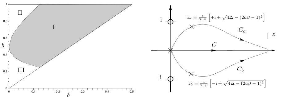
Figure 1: On the left: For values of $b=2\beta a$ and $\delta=2\beta a\Delta$ in the shaded region (I), the saddle points have non-zero real parts. Otherwise (in regions II and III) the saddle points are on the imaginary axis. The boundary of the shaded area on the right hand side ($b=2\delta$) corresponds to (39). On the right: The complex saddle points ($0,\,z_{a},\,z_{b}$) of $q_{a}$ and $q_{b}$ when ($b$, $\delta$)$\in I$, the original contour along the positive real axis ($C$) and the deformed integration contours ($C_{a}$, $C_{b}$).

Returning to the expression of the differential power of the radiation per unit pion energy, the factor $F^{2}(\beta,\Delta,\xi)$ appearing in (28) is just the square of the expression which appears in (32), therefore

$$\frac{\textnormal{d}P}{\textnormal{d}E_{\pi}} = \frac{{g^{2}}}{\pi}\frac{M_{p}\xi}{\gamma}\int\textnormal{d}\Delta\frac{\beta}{\sqrt{\beta^{2}-a\Delta-\frac{m^{2}/M_{p}^{2}+B/B_{0}}{\gamma^{2}}}}$$ (35)

$$\times \frac{1}{\pi\xi}\sqrt{\frac{1}{4\Delta-(2\beta a-1)^{2}}}\,\left[1+\sin\left(2\xi\Phi_{1}(\beta a,\Delta)+2\Phi_{2}(\beta a,\Delta)\right)\right]\,$$

The strongly oscillating term of the integrand would give ${\cal O}(1/\xi)$ contribution therefore one can neglect it and one finds a simple result which is different from zero for a restricted range of $E_{\pi}/E_{p}$ ($0.25\leq E_{\pi}/E_{p}\leq\gamma^{2}$, for $\gamma^{2}\gg 1$) :

$$\frac{\textnormal{d}P}{\textnormal{d}E_{\pi}} = {\frac{g^{2}}{\pi^{2}}}\frac{M_{p}}{\gamma}\int_{(2\beta a-1)^{2}/4}^{\Delta^{+}}\textnormal{d}\Delta\frac{\beta}{\sqrt{\beta^{2}-a\Delta-\frac{m_{\pi}^{2}/m_{p}^{2}+B/B_{0}}{\gamma^{2}}}}\frac{1}{\sqrt{4\Delta-(2\beta a-1)^{2}}}$$ (36)

$$\approx \frac{g^{2}}{2\pi}\frac{E_{\pi}}{\gamma^{2}},\,\,\,\,\,\,\textrm{if}\,\qquad\frac{1}{4}\leq\frac{E_{\pi}}{E_{p}}\leq\gamma^{2}\,.$$

This simple result can be used actually only for $E_{\pi}<E_{p}$ since the energy of the radiated pion cannot exceed the energy of its parent proton. The result is compared next with the results of [14] and [10].

5 Numerical results

Figure 2: The differential radiation power per unit $\pi^{+}$ energy for different proton energies in comparison with the $\pi_{0}$ radiation given by [14] for strong ($B=10^{16}$ G) magnetic fields.

In figure 2 we plotted the above expression and the corresponding $\pi_{0}$ spectra for different proton energies at $B=10^{16}$ G. In this plot we restrict the emitted pion energy to the physically interesting region ($E_{\pi}<E_{p}$) as in [14]. It is interesting that the width of spectrum in our case is independent of the proton energy (in logarithmic scale) in contrast to the case of $\pi_{0}$ emission. This behaviour is obvious from the very simple expression (36), and this is the consequence of the large $\xi$ asymptotic form of the Laguerre polynomial (32), which becomes exponentially small when $\beta=E_{\pi}/E_{p}$ goes over from region I to region II or III (see figure 1). The location of the intersection of the boundary of region I and of the integration range of (36) is independent of $\xi$ (and $B$) and lies at $E_{\pi}/E_{p}=1/4$. In our approximation the slope of the spectrum variation is infinite at $E_{\pi}/E_{p}=1/4$ due to the very different behaviour of the Laguerre polynomials in regions I and III. As a matter of fact, our saddle point analysis is not valid in a very small vicinity of the boundary of regions I and II. due to the fact that the second derivative of $q_{a,b}$ in (31) tends to zero when $\beta,\,\Delta$ reach the boundary. The detailed investigation of the saddle point structure of Laguerre polynomials shows that the width of this “transition” region is $\approx 1/\xi$, and the slope of the spectrum at $E_{\pi}/E_{p}=1/4$ in figure 2 is proportional to $\xi$ (logarithmic scale!).

Another interesting property of the $\pi^{+}$ radiation is that the total emitted pion energy (integral of the expression (36) over $E_{\pi}$) is independent of the magnetic field in our approximation. This $B$ independence is also shown in [14] for the $\pi^{0}$ radiation at large magnetic fields and/or proton energy, in contrast with [10], where the total emitted $\pi^{0}$ energy is proportional to $B^{2}$. The origin of the difference between these two results (although both papers are based on the same semiclassical treatment of the $\pi_{0}$ radiation, calculated in [10]) is that in [14] the differential power of radiation is integrated over $E_{\pi}$ from $m_{\pi}$ to $E_{p}$, while in [10] the integration range is infinite, and the dominant contribution of emitted energy comes from the unphysical ($E_{\pi}>E_{p}$) region of the spectrum in case of large $B$ and/or $E_{p}$.

6 Discussion

The prospective astrophysical interest of the very high energy neutrino source discussed in this paper depends on the simultanous occurrence of very strong magnetic fields and very energetic (e.g. $100$ TeV) protons. Different propositions put proton acceleration at different distances from the surface of the neutron core, therefore the actual magnitude of the magnetic field strength might vary strongly. Most optimistic is the so-called “light-cylinder” accelerator mechanism, which in fast rotating objects can be located close to the surface. In this case the magnetic field strength is not much weaker than that directly measurable on the surface. Since surface keV-photons are necessarily present a concurrence between resonant photoproduction of charged pions (from the decay of $\Delta^{+}$) and non-resonant synchrotron radiation-like-production (4) should be envisaged. There could be 10-20 magnetars in our galaxy, with the great observational advantage that their activity is not restricted to only a few minutes, like in case of GRB’s. Assuming some well-defined galactic distribution for these objects, one combines it with the neutrino luminosity of single objects to estimate the muon flux generated by $\nu$-detection in ice.

Appendix

We present below a detailed derivation of the asymptotic behaviour of (31) when $\xi>>1$. The notation looks somewhat simpler if one goes back to the original Landau level wave functions

$$F(\beta,\Delta,\xi)=R^{\mu}_{n}\left(\frac{\mu}{2b}\right),\qquad b\equiv a\beta.$$ (37)

Relations between the variables $\Delta=n/\xi,\mu=2b\xi$ were used in the main text. The integral representation of this function has now the following form:

$$R^{\mu}_{n}\left(\frac{\mu}{2b}\right) = \frac{1}{\sqrt{\Gamma(n+1)\Gamma(n+\mu+1)}}\exp\left(\frac{\mu}{4b}\right)\left(\frac{\mu b}{2}\right)^{n+\mu/2+1}$$ (38)

$$\times {\int_{0}^{\infty}\mathrm{d}x\exp\left(\mu\left[-xb/2+(\delta+1/2)\ln x\right]\right)J_{\mu}(\mu\sqrt{x})}\,,$$

where a new integration variable is introduced instead of the variable appearing in (30) and also a new parameter is defined:

$$k=x\frac{\mu b}{2},\qquad 0<\delta\equiv\frac{n}{\mu}<\frac{b}{2}\,.$$ (39)

In our application $\mu$ is large, one can use the asymptotic form of the Bessel functions given by 9.3.2 and 9.3.3 of [15],

$$J_{\mu}(\mu\sqrt{x})\!=\!\!\frac{1}{\sqrt{2\pi\mu}}\times\left\{\begin{array}[]{l}\frac{2}{\sqrt{{\tan}K_{1}}}\cos(\mu(\tan K_{1}-K_{1})-\pi/4),\,\,\,\,\,\textrm{if }x>1\\ \frac{1}{\sqrt{\tanh K_{2}}}\exp(\mu(\tanh K_{2}-K_{2})),\,\,\quad\quad\textrm{if }x<1\end{array}\right.\!\!,$$ (40)

where

$$\begin{array}[]{l}\cos K_{1}=\sqrt{1/{x}},\\ \tan K_{1}=\sqrt{x-1},\end{array}\qquad\begin{array}[]{l}\cosh K_{2}=\sqrt{1/{x}},\\ \tanh K_{2}=\sqrt{1-x}\,,\end{array}$$ (41)

Therefore (38) is broken up into the sum of two integrals:

$$R^{\mu}_{n}\left(\frac{\mu}{2b}\right)=N(I_{1}+I_{2}),$$ (42)

where

$$I_{1} = \!\int_{1}^{\infty}\!\!\mathrm{d}x\frac{2}{(x-1)^{1/4}}\exp\left(\mu\left[-\frac{xb}{2}+(\delta+\frac{1}{2})\ln x\right]\right)$$ (43)

$$\times \cos\left(\mu\left[\sqrt{x-1}-\mathrm{acos}\,\left(\frac{1}{\sqrt{x}}\right)\right]-\frac{\pi}{4}\right),$$

$$I_{2} = \!\int_{0}^{1}\mathrm{d}x\frac{1}{(1-x)^{1/4}}\exp\left(\mu\left[-\frac{xb}{2}+(\delta+\frac{1}{2})\ln x+\sqrt{1-x}-\mathrm{acosh}\,\left(\frac{1}{\sqrt{x}}\right)\right]\right)\!,$$ (44)

$$N = \frac{1}{\sqrt{2\pi\mu\Gamma(n+1)\Gamma(n+\mu+1)}}\exp\left(\frac{\mu}{4b}\right)\left(\frac{\mu b}{2}\right)^{n+\mu/2+1}.$$ (45)

Moreover, $N$ can be replaced in the asymptotic regime using Stirling’s formula for the $\Gamma$-functions,

$$N \approx \frac{1}{2\pi\sqrt{\mu}}\exp\left[\mu\left(\frac{1}{4b}+\frac{1}{2}\right)+n+1+\frac{\mu}{2}\ln\left(\frac{\mu b}{2(n+\mu+1)}\right)\right.$$ (46)

$$+ \left.n\ln\left(\frac{\mu b}{2\sqrt{n+1}\sqrt{n+\mu+1}}\right)+\ln\left(\frac{\mu b}{2\left(n+\mu+1\right)^{1/4}\left(n+1\right)^{1/4}}\right)\right].$$

Now we can proceed with the evaluation of $I_{1}$. The method will be similar also for $I_{2}$, and will be just stated after the discussion of the case of $I_{1}$. One changes once more the integration variable in (43),

$$I_{1}=2\exp\left(-\frac{\mu b}{2}\right)\int_{0}^{\infty}\mathrm{d}z\sqrt{z}\left[\exp\left(\mu q_{a}(z)-\mathrm{i}\frac{\pi}{4}\right)+\exp\left(\mu q_{b}(z)+\mathrm{i}\frac{\pi}{4}\right)\right],$$ (47)

where one introduces

$$x=z^{2}+1\,\leftrightarrow(x-1)^{1/4}=\sqrt{z}\,,$$ (48)

and

$$q_{a}(z) = -z^{2}\frac{b}{2}+\left(\delta+\frac{1}{2}\right)\ln(z^{2}+1)+\mathrm{i}\sqrt{z^{2}}-\mathrm{i}\,\mathrm{acos}\sqrt{\frac{1}{z^{2}+1}},$$ (49)

$$q_{b}(z) = -z^{2}\frac{b}{2}+\left(\delta+\frac{1}{2}\right)\ln(z^{2}+1)-\mathrm{i}\sqrt{z^{2}}+\mathrm{i}\,\mathrm{acos}\sqrt{\frac{1}{z^{2}+1}}.$$ (50)

In (47) the integrand can be continued analytically into the complex $z$ plane, which allows the use of the method of steepest descent and stationary phase for the evaluation of the integral (saddle point approximation in the complex plane). For $\mathbf{Re}\,z>0$,

$$q_{a,b}(z)=-z^{2}\frac{b}{2}+\left(\delta+\frac{1}{2}\right)\ln(z^{2}+1)\pm\mathrm{i}{z}\mp\frac{1}{2}\ln\frac{1+\mathrm{i}z}{1-\mathrm{i}z}.$$ (51)

The saddle points are determined by the zeros of the derivative $q_{a,b}^{\prime}(z)$,

$$q_{a,b}^{\prime}(z)=-bz+\frac{(2\delta+1)z}{z^{2}+1}\pm\mathrm{i}\mp\mathrm{i}\frac{1}{z^{2}+1}{=}0.$$ (52)

The location of the solutions on the complex $z$–plane depends on the values of $\delta$ and $b$: there are actually three distinct regions in the ($b$ – $\delta$) plane (see the left hand side of figure 1). We listed in table 1 the solutions of the saddle equations which correspond to the different values of ($b$, $\delta$). In the table $z_{1}$, $z_{2}$ denote

$$z_{1}=\frac{1}{2b}\left[\mathrm{i}+\sqrt{8b\delta-(2b-1)^{2}}\right],\quad z_{2}=\frac{\mathrm{i}}{2b}\left[1-\sqrt{(2b-1)^{2}-8b\delta}\right].$$ (53)

	($b,\,\delta$) $\in$ I	($b,\,\delta$) $\in$ II	($b,\,\delta$) $\in$ III
$z_{a}:$	$\left\{0,z_{1}\right\}$	$\left\{0,z_{2}\right\}$,   $(\left|z_{2}\right|<1)$	$\left\{0,z_{2}\right\}$,  $(\left|z_{2}\right|>1)$
$z_{b}:$	$\left\{0,z_{1}^{\star}\right\}$	$\left\{0,z_{2}^{\star}\right\}$,   $(\left|z_{2}\right|<1)$	$\left\{0,z_{2}^{\star}\right\}$,   $(\left|z_{2}\right|>1)$

Table 1: The location of saddle points of $q_{a}$, $q_{b}$ are $z_{a}$, $z_{b}$ correspondingly. The $z_{1}$ and $z_{2}$ are given in (53).

It is interesting that, the “trivial”$z=0$ saddle point is present in each region. However, when one continues analytically also the integrand of $I_{2}$ into the complex plane one finds that its contribution exactly cancels the contribution of the $z=0$ saddle point of $I_{1}$. Hence it is enough to handle $I_{1}$ with its non trivial saddle points. The integration contours which are displayed on the right hand side of figure 1 correspond to region I.

For the actual evaluation with help of the saddle point technique let us recall that its general strategy tells us that we have to deform the integration contour of $I_{1}$ in order the integration path passes over the saddle point (see the r.h.s. of figure 1) because the dominant contribution of the integral comes from the neighbourhood of the saddle point. Near the saddle point $q_{a,b}(z)$ can be approximated by their second order Taylor expansions around the saddle point,

$$q(z)=q(z_{s})+\frac{1}{2}\left.q^{\prime\prime}\right|_{z_{s}}\left(z-z_{s}\right)^{2}=q(z_{s})-D\frac{\tau^{2}}{2},$$ (54)

where $z_{s}$ denotes the corresponding saddle point and

$$D=\left|q^{\prime\prime}(z_{s})\right|,\quad\,\,z=z_{s}+\tau\exp\left[\frac{-\mathrm{i}}{2}\left(\mathrm{arctan}\left(\frac{\mathbf{Im\,}q^{\prime\prime}(z_{s})}{\mathbf{Re\,}q^{\prime\prime}(z_{s})}\right)\mp{\pi}\right)\right],\quad\tau\in\mathbf{R}\,.$$ (55)

Practically speaking, the above form of $q_{a,b}$ provides a parameterization ($z(\tau)$) of the integration path near the saddle point in which the argument of the exponential function have constant imaginary part along the parameterized integration contour (stationary phase). Using the above parameterization for an integral of type $I_{1}$, one can write

$$\int_{0}^{\infty}\mathrm{d}z\sqrt{z}\exp\left(\mu q(z)\right)\approx\mathrm{e}^{\mu q(z_{s})}\int_{z_{s}}\mathrm{d}\tau\frac{\mathrm{d}z}{\mathrm{d}\tau}\sqrt{z(\tau)}\exp\left(-\mu D\frac{\tau^{2}}{2}\right)\approx$$

$$\approx\sqrt{z_{s}}\left.\frac{\mathrm{d}z}{\mathrm{d}\tau}\right|_{z_{s}}\mathrm{e}^{\mu q(z_{s})}\int_{-\infty}^{\infty}\mathrm{d}\tau\exp\left(-\mu D\frac{\tau^{2}}{2}\right)=\sqrt{z_{s}}\mathrm{e}^{\mu q(z_{s})}\sqrt{\frac{-2\pi}{\mu q^{\prime\prime}(z_{s})}},$$ (56)

where in the first line the notation $\int_{z_{s}}$ means that the integration range is a small interval near $z_{s},\,(\tau=0)$. In the second line this range is extended to $[-\infty,\,\infty]$ because the contribution to a Gaussian integral is small far away from the saddle point when $\mu$ is large. In addition we write $\sqrt{z_{s}}$ instead of $\sqrt{z}$ since it is a slowly varying function near the saddle point. Higher order terms of the Taylor expansion of $\sqrt{z}$ give $\mathcal{O}(1/\mu)$ corrections.

It can be seen from (56) that the order of magnitude of the integral $I_{1}$ is determined by the real part of $q_{a,b}(z_{s})$, which can be written for the regions $i=$ (I, II, III) in the form $q^{i}_{a}(z^{i}_{s})=R^{i}+\mathrm{i}\Gamma^{i}$, $q^{i}_{b}(z^{i}_{s})=R^{i}-\mathrm{i}\Gamma^{i}$. After some algebra, where one pays attention to the branch cuts of $\exp(\mu q(z_{s}))$ appearing in (56) one can obtain the following explicit expressions for the real and imaginary parts:

$$R^{I}\!\! = \!-\frac{1}{4b}+\frac{b-1-2\delta}{2}+\frac{2\delta+1}{2}\ln\left(1+\delta\right)+\delta\ln\sqrt{\delta^{2}+\delta},$$ (57)

$$R^{II}\!\! = \!-\ln(2)-\frac{1}{4\beta}\left(2b-1-\sqrt{(2b-1)^{2}-8b\delta}\right)+$$ (58)

$$+ \!(\delta+1)\ln\left(2b+1-\sqrt{(2b-1)^{2}-8b\delta}\right)-\delta\ln\left(2b-1-\sqrt{(2b-1)^{2}-8b\delta}\right)\!,$$

$$R^{III}\!\! = \!-\ln(2)-\frac{1}{4b}\left(2b-1+\sqrt{(2b-1)^{2}-8b\delta}\right)+$$ (59)

$$+ \!\!(\delta+1)\ln\left(2b+1+\sqrt{(2b-1)^{2}-8b\delta}\right)\!-\!\delta\ln\left(\left|2b-1+\sqrt{(2b-1)^{2}-8b\delta}\right|\right)\!,$$

$${I^{I}}\!\! = \!\frac{\sqrt{8b\delta-(2b-1)^{2}}}{4b}+\frac{2\delta+1}{2}\mathrm{atan}\,\frac{\sqrt{8b\delta-(2b-1)^{2}}}{2b-1+4b\delta}$$ (60)

$$- \!\frac{1}{2}\mathrm{atan}\,\frac{\sqrt{8b\delta-(2b-1)^{2}}}{2b-1-2b\delta}\,,$$

$${I^{II}}\!\! = \!I^{III}=0.$$ (61)

Using these expressions together with the form of the normalization factor $N$ from (46) and the exponential factor from (47) one obtains that

$$0<R^{II,III}-b/2\approx\mathcal{O}(1),\quad\textrm{ therefore}\quad N\exp\left(\mu(R^{II,III}-b/2\right))\ll 1,$$ (62)

hence $R_{n}^{\mu}(\mu/2b)$ is exponentially small when $b,\,\delta$ are in regions II or III. Unlike in region I, where the exponential factors are cancelled, and the result is surprisingly simple:

$$N^{\prime}\exp\left(R^{I}-\mu\frac{b}{2}\right)\approx\left[\frac{\delta}{\delta+1}\right]^{1/4}.\\$$ (63)

Using (63) in (56) together with the explicit form of $q^{\prime\prime}(z_{s})$, one can obtain the expression (32). This form of the asymptotic behaviour of the Laguerre polynomials is in agreement with the results of [16], where asymptotic analysis of the Laguerre polynomials was derived with help of the generating function of these functions.

References

- [1] IceCube Coll (M. Krasberg) AIP Conf.Proc.867 (2006) 209-216
- [2] U.F. Katz, Nucl. Instr.Meth. A567 (2006) 457
- [3] J.N. Bahcall and P. Mészáros, Phys. Rev. Lett. 85 (2000) 1362
- [4] B. Zhang, Z.G. Dai, P. Mészáros, E. Waxman and A.K. Harding, Ap.J. 595 (2003) 346
- [5] J. Arons, ApJ 589 (2003) 871
- [6] A. Atoyan and C.D. Dermer, Phys. Rev. Lett. 87 (2001) 221102
- [7] P. Blasi, R.I. Epstein and A.V. Olinto, ApJ 533 (2000) L123
- [8] A. Kappes, J. Hinton, C. Stegmann and F.A. Aharonian, ApJ 656 (2007) 870
- [9] E. Waxman and J.N. Bahcall, Phys. Rev. Lett. 78 (1997) 2292
- [10] V.L. Ginzburg and G.F. Zharkov, JETP 47 (1964) 2279
- [11] V.L. Ginzburg and S.I. Sirovatski, Ann. Rev. Astron. Astrophys. 3 (1965) 297
- [12] G.F. Zharkov, J. of Sov. Nucl. Phys. 1 (1965) 173
- [13] A.K. Harding and D. Lai, Repts on Progress in Phys. 69 (2006) 2631
- [14] A. Tokuhisa and T. Kajino Ap.J. 525 (1999) L117
- [15] M.A. Abramowitz and I.A. Stegun, Handbook of Mathematical Functions, Nat. Bur. Stand. Appl. Math. Ser. 55 (1964)
- [16] A.P. Smith, J. Math. Phys. 33 (1992) 1666