Kinetic Energy Density Study of Some
Representative Semilocal Kinetic Energy Functionals

Abstract

There is a number of explicit kinetic energy density functionals for non-interacting electron systems that are obtained in terms of the electron density and its derivatives. These semilocal functionals have been widely used in the literature. In this work we present a comparative study of the kinetic energy density of these semilocal functionals, stressing the importance of the local behavior to assess the quality of the functionals. We propose a quality factor that measures the local differences between the usual orbital-based kinetic energy density distributions and the approximated ones, allowing to ensure if the good results obtained for the total kinetic energies with these semilocal functionals are due to their correct local performance or to error cancellations. We have also included contributions coming from the laplacian of the electron density to work with an infinite set of kinetic energy densities. For all the functionals but one we have found that their success in the evaluation of the total kinetic energy are due to global error cancellations, whereas the local behavior of their kinetic energy density becomes worse than that corresponding to the Thomas-Fermi functional.

I Introduction

Density Functional Theory (DFT) has nowadays a privileged position within the current methods for calculating the electron structure. The theorems of Hohenberg and Kohn Hohenberg and Kohn (1964) show that the ground state of a system of nuclei and electrons can be fully described in terms of its electron density. In fact, the total energy $E[n]$ of the electrons can be written as a functional of the density and the variational minimization of $E[n]$ yields the ground state electron density and its total energy.

The usual procedure within the DFT solves the Kohn-ShamKohn and Sham (1965) (KS) equations for $N$ orbitals, where $N$ is the number of electrons of the system. This KS method allows the partition of the total energy functional in different pieces with distinct physical meanings

$$E[n]=T_{S}[n]+V[n]+J[n]+E_{xc}[n],$$ (1)

where $E[n]$ is the total energy, $V[n]$ is the energy of the electron density allocated in the electric field generated by the nuclei, $J[n]$ is the classical repulsion of the electron density (also called Hartree energy), $T_{S}[n]$ is the kinetic energy of a noninteracting system that yields the same electron density of the interacting one and $E_{xc}[n]$ is a density functional that takes into account the exchange and the correlation (XC) energies. The major part of the kinetic energy, $T_{S}[n]$, is then expressed exactly by means of the KS one-electron orbitals and the small part ($T[n]-T_{S}[n]$) is included in the XC functional, $E_{xc}[n]$, which is the only part of the energy to be approximated. The exact ground-state electron density $n\left(\mathbf{r}\right)$ is the sum of the densities of the KS orbitals, the kinetic energy functional is evaluated exactly through the KS orbitals,Kohn and Sham (1965) and the minimization of the total energy functional (1) becomes the resolution of a set of coupled Schrödinger-like equations for the KS orbitals.

The computational cost of solving the KS equations can be avoided by using $T_{S}$ as a functional depending explicitly on the electron density, instead of constructing the KS orbitals and evaluating the kinetic energy in terms of them. In that case, the computational cost of this orbital-free procedure would scale with the number of electrons (a linear scaling method) and can offer much faster computational times than the KS calculations, allowing to deal with systems that involve several hundred thousands of atoms or more. The ground state of these systems is then calculated through an Euler-Lagrange variational minimization. Moreover, the use of an approximate orbital-free kinetic energy functional, instead of the KS method, makes easier the evaluation of the forces and reduces the computational cost of complex calculations in first-principle molecular dynamics Car and Parrinello (1985). But one of the issues that must be solved about orbital-free kinetic energy functionals is the stability of their numerical solutions, because some functionals have been proved to be linearly stable but nonlinearly unstable (see, e. g., Ref. Blanc and Cances, 2005) and the solution obtained can be meaningless.

As a consequence, the construction of functionals depending explicitly on the density $n\left(\mathbf{r}\right)$ (without any reference to the wave functions) has an undoubted formal interest and an important practical side. Being the analytic dependence of $T_{S}$ on the electron density a rather academic problem for a long time (see reviews in Refs. Parr and Yang, 1989 and Wang and Carter, 2000), the increasingly rapid development of computational chemistry has turn it an interesting topic, from the proposals of new kinetic energy functionalsAlonso and Girifalco (1978); Chacón et al. (1985); García-Gonzalez et al. (1996a, b, 1998a, 1998b); García-González et al. (2000); Wang and Teter (1992); Foley and Madden (1996); Wang et al. (1999); Watson and Carter (2000); Carling and Carter (2003); Zhou et al. (2005) to the study of the kinetic energy densityYang et al. (1996); Sim et al. (2003) and the application to simple systems.Iyengara et al. (2001); Chan et al. (2001); King and Handy (2001)

In order to construct accurate explicit $T_{S}\left[n\right]$ functionals we need to get not only good total energies but also the correct density profiles for the ground state of the total energy functional (Eq. 1) after a fully variational minimization of the energy. For that reason, although common tests to determine the quality of a kinetic energy functional only calculate the energies and density profiles using good densities (i.e., those obtained with accurate methods such as the Hartree-Fock or KS ones) we are interested in studying the quality of the kinetic functionals beyond this limitation. In particular, we think the properties of the kinetic energy density deserve a study by itself, paving the way for understanding when and why functionals are able or not to describe the characteristic quantum properties, like the presence of structure in the density profiles.

This paper presents an extensive study of the kinetic energy densities of a number of semilocal kinetic functionals thanks to the proposal of a quality factor that helps to determine how far from a valid kinetic energy density are the approximated ones.

II The Kinetic Energy Density

The kinetic energy density (KED) can be defined as any function $t_{S}(\mathbf{r})$ that integrates to the exact total kinetic energy,

$$T_{S}[n]=\int d\mathbf{r~{}}t_{S}(\mathbf{r}).$$ (2)

It is clear that such definition does not determine the kinetic energy density uniquely: any function – with the appropriate scaling properties – that integrates to zero in the whole space can be added to any KED to yield another KED, and an infinite number of new valid KEDs can be defined by multiplying this function by any coefficient. The non uniqueness of the kinetic energy density has been studied in the literature.Yang et al. (1996); Sim et al. (2003)

Within the KS method, an orbital-based KED can be obtained in terms of the KS orbitals. Two main definitions are commonly used in the literature. The first definition has the advantage of being positive everywhere, because it is calculated through the squared gradient of the orbitals of an $N$-electron system (atomic unit will be used in this paper):

$$t_{S}^{I}(\mathbf{r})=\frac{1}{2}\sum_{i=1}^{N}\left|\nabla\phi_{i}(\mathbf{r})\right|^{2},$$ (3)

where $\phi_{i}(\mathbf{r})$ is the $i$th KS orbital. A second definition can be obtained using the kinetic energy operator in the way it appears in the KS equations, yielding a non positive definite function:

$$t_{S}^{II}(\mathbf{r})=-\frac{1}{2}\sum_{i=1}^{N}\phi_{i}^{\ast}(\mathbf{r})\nabla^{2}\phi_{i}(\mathbf{r}).$$ (4)

Functions $t_{S}^{I}$ and $t_{S}^{II}$ are related through the laplacian of the electron density,

$$t_{0}(\mathbf{r})=\nabla^{2}n(\mathbf{r}),$$ (5)

as

$$t_{S}^{I}(\mathbf{r})-t_{S}^{II}(\mathbf{r})=\frac{1}{4}t_{0}(\mathbf{r}).$$ (6)

They have different local properties, but both of them are valid definitions for KED because they integrate to the same total kinetic energy since the integral of $t_{0}(\mathbf{r})$ over the whole space is zero. In finite systems the electron density decays exponentially and the divergence theorem can be used to transform the integral over the space into a surface integral, $\int_{V}d\mathbf{r\nabla}^{2}n(\mathbf{r})=\int_{S}d\mathbf{S\nabla}n(\mathbf{r})$. The gradient of the electron density decays faster than the growth of the surface (which is proportional to $r^{2}$) and the integral is zero. For extended systems, but periodic, the last integral is extended over the surface of the unit cell of the periodic system; the gradients in opposites sides of the cell cancel one each other, and the surface integral has also a zero value.

We must remark that, besides the interest of the study of the intrinsic properties of the KED, some new XC density functionals have been proposed using the KED.Boese and Handy (2002); Ernzerhof et al. (2002); Maximoff et al. (2002)

III Simple kinetic energy density functionals

III.1 The First Functional Approximations.

The first explicit kinetic energy density functional formulated was the Thomas-Fermi (TF) approximation,Thomas (1927); Fermi (1927) where each point of an inhomogeneous electron system with density $n(\mathbf{r})$ contributes to the kinetic energy as any point in an homogeneous one with the same electron density, $n_{0}=n(\mathbf{r})$. We then get the TF functional

$$T_{TF}[n(\mathbf{r})]=\int d\mathbf{r}C_{TF}n^{5/3}(\mathbf{r}),$$ (7)

where $C_{TF}=\frac{3}{10}(3\pi^{2})^{2/3}$ is the TF constant. By construction, this functional is exact for homogeneous systems and a good approximation for systems close to the free electron gas.March (1983); Lieb (1981) But this functional gives, in general, poor results when applied to atoms or molecules, and the density profiles obtained in a variational minimization show no quantum effects. For atoms, in fact, no shell structure is obtained and the errors in the total kinetic energy are about 10%. This relative error is also obtained when the functional is applied using good densities.

Another explicit kinetic energy density functional is the von Weizsäcker (vW) $T_{vW}[n]$ functional, constructed to be exact for one or two electrons in the same spacial state.Weizsacker (1935) The most usual form in which functional is found in the literature is

$$T_{vW}[n]=\frac{1}{8}\int{\frac{|\mathbf{\nabla}n(\mathbf{r})|^{2}}{n(\mathbf{r})}d\mathbf{r}},$$ (8)

but can also rewritten in other ways that yield the same total kinetic energy. Being the functional exact for single orbital systems, it gives the correct KED when the contribution of a given orbital to the electron density is much larger than all the other orbitals. For the same reason, for those regions in space that are very close or very far away from the positions of the nuclei, this functional also gives the correct KED. Finally, $T_{vW}[n]$ is exact in regions with large variations of the electron density. But when applied to general systems this functional yields large errors. So, the variational minimization for atoms gives no shell structures and the relative errors increase a lot when the number of electrons grows, getting energies of a different order of magnitude than the exact ones for atoms with a large number of electrons.

A very interesting functional can be obtained as a combination of the TF and vW functionals, the so called second order gradient expansion approximation (GEA2), constructed as:Kirzhnits (1957)

$$T_{S}^{GEA2}[n] =T_{TF}[n]+\frac{1}{9}T_{vW}[n]$$

$$=C_{TF}\int{n(\mathbf{r})^{5/3}d\mathbf{r}}+\frac{1}{72}\int{\frac{|\mathbf{\nabla}n(\mathbf{r})|^{2}}{n(\mathbf{r})}d\mathbf{r}}$$ (9)

$$=C_{TF}\int{d\mathbf{r}n(\mathbf{r})^{5/3}}\left[1+\frac{1}{72C_{TF}}\left|\frac{\mathbf{\nabla}n(\mathbf{r})}{n^{4/3}(\mathbf{r})}\right|^{2}\right].$$

This functional gives the correct kinetic energies for systems with slow varying electron densities. Density profiles obtained in the variational minimization of the total energy with the GEA2 approximation show the same pathologies as the previous functionals, but when applied using good electron densities the error in the total energy is only about 1% for a number of very different systems. This error is clearly too big for chemical precision, but is quite small for common orbital-free kinetic energy density functionals.Iyengara et al. (2001)

III.2 The Generalized Gradient Approximations.

In this paper we make a comprehensive study of the kinetic energy density functionals that can be expressed within the Generalized Gradient Approximation (GGA), which allows a general form for those semilocal functionals that only depend on the electron density and its gradient. Any semilocal functional of this kind can be written as

$$T_{S}^{GGA}[n(\mathbf{r})]=\int d\mathbf{r}t_{TF}\left(\mathbf{r}\right)F_{enh}(s(\mathbf{r})),$$ (10)

where $t_{TF}\left(\mathbf{r}\right)=C_{TF}n^{5/3}(\mathbf{r})$ is the KED corresponding to the TF functional and $F_{enh}(s(\mathbf{r}))$ is the so-called enhancement factor, that depends on the adimensional variable

$$s(\mathbf{r})=\frac{\left|\mathbf{\nabla}n(\mathbf{r})\right|}{n^{4/3}(\mathbf{r})}.$$ (11)

The quantity $s(\mathbf{r})$ is called the reduced density gradient and has a clear physical interpretation, because it controls the speed of the variation of the electron density. Large values of $s(\mathbf{r})$ correspond to fast variations in the electron density and small values to slow ones; a zero value indicates a region of the space where the electron density has no variation.

The mathematical form of the enhancement factor determines the functional and authors have proposed many different forms for the enhancement factor. In this paper, the following set of semilocal functionals have been selected.

1. Thomas–Fermi functional (TF).Thomas (1927); Fermi (1927) When the enhancement factor has a constant value of $1$, the TF functional is recovered,

$$F_{TF}(s(\mathbf{r}))=1.$$

2. Second order gradient expansion approximation (GEA2).Kirzhnits (1957) This approximation is a particular case of the GGA approximations, obtained with the expression:

$$F_{GEA2}(s(\mathbf{r}))=\left[1+\frac{1}{72C_{TF}}s(\mathbf{r})^{2}\right].$$

There are some functionals constructed as a linear combination of the TF functional and the vW functional. We cite now some of them.

3. Thomas–Fermi + $\frac{1}{5}$ von Weizsäcker (TF$\mathbf{5}$W). In this case the contribution of the vW functional is weighted by a prefactor $1/5$, Yonei and Tomishima (1965); Tomishima and Yonei (1966); Yonei (1967, 1982); Gross and Dreizler (1979); Berk (1983); Stich et al. (1982); Govind et al. (1994); Chan et al. (2001)

$$F_{TF5W}(s(\mathbf{r}))=\left[1+\frac{1}{40C_{TF}}s(\mathbf{r})^{2}\right].$$

4. Thomas–Fermi + von Weizsäcker (TFvW).Yonei (1967) The combination involving both the full Thomas-Fermi and von Weizsäcker functionals is theoretically interesting but in practical applications largely overestimate the kinetic energy,

$$F_{TFvW}(s(\mathbf{r}))=\left[1+\frac{1}{8C_{TF}}s(\mathbf{r})^{2}\right].$$

5. Thomas–Fermi + $\frac{b}{9}$ von Weizsäcker (TF$\mathbf{9}$W). A modification of GEA2 can be written with the introduction of a parameter $b$ that modifies the contribution of the gradient correction. Several values of $b$ have been used by different authors. For this work we have chosen a value of $b=1.067$.Thakkar (1992)

$$F_{TF9W}(s(\mathbf{r}))=\left[1+\frac{b}{72C_{TF}}s(\mathbf{r})^{2}\right].$$

6. $N$-dependent Thomas–Fermi functional (TF-$\mathbf{N}$).Thakkar and Pedersen (1990) Several functionals have been developed as modifications of the TF functional by including a prefactor that depends on the number of electrons $N$. For this work we have chosen:

$$F_{TF-N}(s(\mathbf{r}))=\left(1+\frac{0.313}{N^{1/3}}-\frac{0.187}{N^{2/3}}\right),$$

that usually provides better values for the kinetic energies than those obtained with the TF functional.

7. Pearson functional (Pear).Pearson (1982) This functional, a modification of the GEA2 approximation that follows the idea presented by Pearson and Gordon,Pearson and Gordon (1985) is constructed in such a way that the gradient correction takes only into account the regions of the space where the density varies slowly. This can be done with the introduction of a cut-off that depends on the value of the reduced gradient $s$. A sharp cutoff usually introduces numerical problems and a functional with a smooth cutoffPearson (1982) is proposed with the enhancement factor:

$$F_{Pear}[n]=\int{d\mathbf{r}}\left[1+\frac{1}{1+\left[s/\zeta\right]^{6}}\frac{1}{72C_{TF}}s(\mathbf{r})^{2}\right],$$

where $\zeta$ is a parameter that Pearson and Gordon fixed as $\zeta=1$, the optimum value for fitting to atomic Hartree-Fock kinetic energies. This functional form prevents the contributions of the gradient expansions coming from regions where fast variations of the electron density occur.

8. DePristo–Kress functional (DK).Depristo and Kress (1987a) These authors introduce a mathematical form based on a Padé-type approximation that is able to recover different desirable limits:

$$F_{DK}(s(\mathbf{r}))=\frac{9b_{3}x^{4}+a_{3}x^{3}+a_{2}x^{2}+a_{1}x+1}{b_{3}x^{3}+b_{2}x^{2}+b_{1}x+1},$$

where

$$x=\frac{(s(\mathbf{r}))^{2}}{72C_{TF}}.$$

This functional is equivalent to GEA2 for slowly varying densities – small values of $s$ – and equivalent to the von Weizsäcker functional for fast varying densities – large values of $s$ –. The parameters of the functional ($a_{1}=0.95$, $a_{2}=14.28111$, $a_{3}=-19.5762$, $b_{1}=-0.05$, $b_{2}=9.99802$, $b_{3}=2.96085$) were obtained by fitting the results of the functional to atomic Hartree-Fock kinetic energies:

9. Lee–Lee–Parr functional (LLP).Lee et al. (1991) These authors have used the same mathematical form of an enhancement factor for the exchange functional for constructing the kinetic energy density functional

$$F_{LLP}(s(\mathbf{r}))=\left[1+\frac{b\left[s(\mathbf{r})\right]^{2}}{1+c\left[s(\mathbf{r})\right]\arcsin(s(\mathbf{r}))}\right],$$

where the parameters have the values $b=0.0044188$ and $c=0.0253$.

10. Ou-Yang – Levy 1 functional (OL1).Ou-Yang and Levy (1991) Following the nonuniform coordinate scaling requirement for the kinetic energy density functional,Ou-Yang and Levy (1990) these authors suggest these two new functional forms:

$$F_{OL1}(s(\mathbf{r}))=1+\frac{1}{72C_{TF}}\left[s(\mathbf{r})\right]^{2}+d\left[s(\mathbf{r})\right],$$ (12)

where $d=0.00187$, and

11. Ou-Yang – Levy 2 functional (OL2).Ou-Yang and Levy (1991)

$$F_{OL2}(s(\mathbf{r}))=1+\frac{1}{72C_{TF}}\left[s(\mathbf{r})\right]^{2}+\frac{D\left[s(\mathbf{r})\right]}{1+2^{5/3}\left[s(\mathbf{r})\right]},$$

with $D=0.0245$.

12. Thakkar functional (Thak).Thakkar (1992) In a review of many semilocal functionals, Thakkar proposed a new one as a conjoint of the mathematical forms of the most successful functionals:

$$F_{Thak}(s(\mathbf{r}))=1+\frac{b\left[s(\mathbf{r})\right]^{2}}{1+c\left[s(\mathbf{r})\right]\arcsin[s(\mathbf{r})]}-\frac{D\left[s(\mathbf{r})\right]}{1+2^{5/3}\left[s(\mathbf{r})\right]},$$

with the parameters: $b=0.0055$, $c=0.0253$ and $D=0.072$.

As was commented before, Lee, Lee and Parr argued that the enhancement factors used for the GGA XC energy functionals can also be used for the development of kinetic energy functionals. The next five functionals, formulated following that approach, were proposed by Lacks and Gordon.Lacks and Gordon (1994)

13. Becke 86A functional (B86A).Becke (1986a)

$$F_{B86A}(s(\mathbf{r}))=1+0.0039\frac{\left[s(\mathbf{r})\right]^{2}}{1+0.004\left[s(\mathbf{r})\right]^{2}}.$$

14. Becke 86B functional (B86B).Becke (1986b)

$$F_{B86B}(s(\mathbf{r}))=1+0.00403\frac{\left[s(\mathbf{r})\right]^{2}}{\left(1+0.007\left[s(\mathbf{r})\right]^{2}\right)^{4/5}}.$$

15. DePristo–Kress 87 functional (DK87).Depristo and Kress (1987b)

$$F_{DK87}(s(\mathbf{r}))=1+$$

$$\frac{7}{324\left(18\pi^{4}\right)^{1/3}}\left[s(\mathbf{r})\right]^{2}\frac{1+0.861504s(\mathbf{r})}{1+0.044286\left[s(\mathbf{r})\right]^{2}}.$$

16. Perdew–Wang 86 functional (PW86).Perdew and Yue (1986)

$$F_{PW86}(s(\mathbf{r}))=1+1.296\left[s(\mathbf{r})\right]^{2}+14\left[s(\mathbf{r})\right]^{4}+0.2\left[s(\mathbf{r})\right]^{61/15}.$$

17. Perdew–Wang 91 functional (PW91).Perdew et al. (1992)

$$F_{PW91}(s(\mathbf{r}))=$$

$$\frac{1+a_{1}s(\mathbf{r})\arg\sinh\left(b\left[s(\mathbf{r})\right]\right)+\left[a_{2}-a_{3}e^{-100\left[s(\mathbf{r})\right]^{2}}\right]}{1+as(\mathbf{r})\arg\sinh\left(b\left[s(\mathbf{r})\right]\right)+a_{4}\left[s(\mathbf{r})\right]^{2}}.$$

with $a_{1}=0.19645$, $a_{2}=0.2747$, $a_{3}=0.1508$, $a_{4}=0.004$ and $b=7.7956$.

18. Lacks–Gordon functional (LG94). In their extensive study of the kinetic energy density functionals,Lacks and Gordon (1994) these authors made their own contribution with the formulation of a new one, based on a previous exchange functional of the same authors developed by fitting exchange energies of atoms and ions, as well as the correct behavior of the exchange energy for small $s(r)$:

$$F_{LG94}(s(\mathbf{r}))=\left[\frac{1+a_{2}\left[s(\mathbf{r})\right]^{2}+a_{4}\left[s(\mathbf{r})\right]^{4}+a_{6}\left[s(\mathbf{r})\right]^{6}+a_{8}\left[s(\mathbf{r})\right]^{8}+a_{10}\left[s(\mathbf{r})\right]^{10}+a_{12}\left[s(\mathbf{r})\right]^{12}}{1+10^{-8}\left[s(\mathbf{r})\right]^{2}}\right]^{b},$$

with $a_{2}=\left(10^{-8}+0.1234\right)/0.024974$, $a_{4}=29.790$, $a_{6}=22.417$, $a_{8}=12.119$, $a_{10}=1570.1$, $a_{12}=55.944$ and $b=0.024974$.

19. von Weizsäcker functional (vW).Weizsacker (1935) The vW functional can also be written as a semilocal functional if we choose the enhancement factor:

$$F_{vW}(s(\mathbf{r}))=\frac{1}{8C_{TF}}s(\mathbf{r})^{2}.$$

20. Acharya et al. functional (ABSP).Acharya et al. (1980) Acharya, Bartolotti, Sears, and Parr proposed a functional with the full vW functional, introducing a TF contribution weighted by a prefactor depending on the electron number $N$:

$$F_{ABSP}[n]=\frac{1}{8C_{TF}}s(\mathbf{r})^{2}+\left(1-\frac{1.412}{N^{1/3}}\right).$$

21. Gázquez–Robles functional (GR).Gázquez and Robles (1982) Following the same spirit of the previous functional, Gázquez and Robles developed another one, with a more complicated form for the weight of the TF functional:

$$F_{GR}[n]=\frac{1}{8C_{TF}}s(\mathbf{r})^{2}+\left(1-\frac{2}{N}\right)\left(1-\frac{1.303}{N^{1/3}}+\frac{0.029}{N^{2/3}}\right).$$ (13)

IV Measurement of the Distance Between two Kinetic Energy Densities.

As the KED can be evaluated by using the KS orbitals, we may think that every approximate functional yields an approximation to the KED by simply defining it as the integrand $t_{S}^{func}(\mathbf{r})$ that appears in the expression of the functional:

$$T_{S}^{func}[n]=\int d\mathbf{r~{}}t_{S}^{func}(\mathbf{r}).$$ (14)

As the main aim of this paper is to know, in a quantitative way, how the semilocal functionals are able to reproduce the KED, we need to define a measure of the closeness between the orbital-based and approximated orbital-free KED distributions, i.e. we must find an efficient and reasonable measure of the distances between distributions. Some distances between probability distributions have been defined, most of them to be used for normalized and positive definite distributions. The electron density is normalized and positive, but the KEDs are no normalized and they are not, in general, positive definite (note that the second definition of the KS KED has always negative values in some regions of the space). For these reasons those distances are not appropriate in our case. But the absolute value norm, being the absolute value of the difference between two distributions integrated over the whole space, is a measure of the accumulated local error of the KED,

$$\epsilon=\int d\mathbf{r}\left|t_{S}(\mathbf{r})-t_{S}^{func}(\mathbf{r})\right|,$$ (15)

where $t_{S}(\mathbf{r})$ is a valid distribution of KED and $t_{S}^{func}(\mathbf{r})$ an approximated one. This definition satisfies the three desirable requirements for a distance: it is positive definite, is symmetric and verifies the triangular inequality.

The defined measure $\epsilon$ depends on the size of the system, because the total kinetic energy has a nonlinear dependence with the number of electrons (the kinetic energy of neon is more than two hundred times the kinetic energy of hydrogen). In order to get a measure that does not depend so much on the size of the system we divide $\epsilon$ by the exact total kinetic energy. In this way, we propose a quality factor $\sigma$ for a KED as

$$\sigma=\frac{\epsilon}{T_{S}[n]}.$$ (16)

With this definition, the bigger the difference between the distributions is the larger the value of $\sigma$ becomes, and $\sigma$ is zero for two identical KEDs. Note that the value of $\sigma$ can be interpreted as the amount of the approximated KED that is misplaced when compared to the distribution of the orbital-based KED. With this factor $\sigma$ we are going to test whether the good results obtained for the total kinetic energies with the GGA functionals are due to their correct local KED or to error cancellations among different regions of the space.

V Electron Densities for Light Atoms

In order to clarify the quality of the KED each approximate functional yields, we want to use good enough atomic electron densities to evaluate our semilocal functionals.

We initially tried commercial software that performs KS calculations and outputs the orbitals used; in that way the related electron density, the KED and the total kinetic energy can be evaluated. But we decided to avoid the use of these codes for several reasons. Firstly, the behavior of any XC functional leads to a bad decay of the density in the outer region of the atom, reflecting some problems in the quality of the KS orbitals, their density and in the KED. More importantly, when using a basis set of gaussians, several gaussians are generally needed to approximate one Slater-like KS orbital. As a result, changes in the slope of the KS orbitals appear; that could not noticeable by simple inspection but, when the careful numerical evaluation of the laplacian of the density is done, spurious structure arises. So, when the laplacian of the density is numerically evaluated one must be cautious with the use of a gaussian basis set. Furthermore, gaussian basis set are unable to give a good description of both the cusps of the density in the positions of the nuclei and the decay of the orbitals far away from them.

For that reasons, we have decided to use Slater orbitals for the light atoms. They only approximately describe the KS orbitals but all the aforementioned pathologies will not appear (there are no spurious oscillations, no cut-offs and correct cusp conditions and decay of the orbitals can be achieved). There are several sets of values of exponents for the Slater orbitals, with only small differences between them; Table 1 presents our choice of parametersAtkins (1997); Clementi and Raimondi (1963) for the ten first atoms.

	H	He	Li	Be	B	C	N	O	F	Ne
1s	1	1.6875	2.6906	3.6848	4.6795	5.6727	6.665	7.6579	8.6501	9.6421
2s			1.2792	1.912	2.5762	3.2166	3.8474	4.4916	5.1276	5.7584
2p					2.4214	3.1358	3.834	4.4532	5.1000	5.7584

Table 1: Values of the effective charge, $Z_{eff}$.

VI Total Kinetic Energies

We have performed total energy calculations for twenty one functionals, using the densities corresponding to the Slater orbitals with parameters given in Table 1.

The relative errors for the total kinetic energies are presented in Table 2. We also show the average of the absolute values of the errors for every functional. To add more information, the dispersion of data is displayed under the label “Range”, where we give the statistical range, i.e., the length of the interval which includes all the former data. When the value of the range is larger than the average we can think the average could be meaningless. All the tables of this paper will be presented this way (in each case, for the relative error, for the values of $\sigma$, etc.).

	H	He	Li	Be	B	C	N	O	F	Ne	Ave	Range
TF	-0.082	-0.082	-0.085	-0.091	-0.097	-0.095	-0.085	-0.090	-0.087	-0.077	0.087	0.020
GEA2	0.029	0.029	0.023	0.013	0.003	0.000	0.006	-0.003	-0.003	0.004	0.011	0.032
TF5W	0.118	0.118	0.109	0.097	0.083	0.077	0.079	0.067	0.064	0.068	0.088	0.054
TFvW	0.918	0.918	0.887	0.846	0.800	0.762	0.736	0.695	0.667	0.648	0.788	0.269
TF9W	0.036	0.036	0.030	0.020	0.010	0.007	0.013	0.003	0.003	0.009	0.017	0.034
TF-N	0.034	0.038	0.031	0.021	0.011	0.010	0.018	0.010	0.011	0.020	0.020	0.028
Pear	-0.070	-0.070	-0.074	-0.079	-0.085	-0.083	-0.073	-0.078	-0.075	-0.064	0.075	0.021
DK	0.031	0.031	0.016	-0.003	-0.011	-0.010	-0.001	-0.007	-0.005	0.005	0.012	0.042
LLP	0.023	0.023	0.018	0.011	0.002	0.001	0.008	0.000	0.001	0.008	0.010	0.022
OL1	0.039	0.039	0.032	0.023	0.012	0.010	0.016	0.006	0.006	0.013	0.020	0.033
OL2	0.036	0.036	0.029	0.020	0.009	0.007	0.013	0.004	0.004	0.011	0.017	0.032
Thak	0.026	0.026	0.022	0.015	0.006	0.005	0.011	0.004	0.004	0.011	0.013	0.022
B86A	0.023	0.023	0.019	0.013	0.004	0.003	0.010	0.002	0.003	0.010	0.011	0.021
B86B	0.049	0.049	0.045	0.038	0.028	0.026	0.033	0.025	0.025	0.032	0.035	0.025
DK87	0.030	0.030	0.026	0.019	0.010	0.009	0.015	0.008	0.008	0.015	0.017	0.022
PW86	0.020	0.020	0.016	0.009	0.001	0.000	0.007	-0.001	0.000	0.008	0.008	0.021
PW91	0.026	0.026	0.021	0.014	0.005	0.003	0.009	0.001	0.001	0.008	0.011	0.025
LG94	0.024	0.024	0.020	0.013	0.005	0.004	0.010	0.003	0.003	0.011	0.012	0.021
vW	0.000	0.000	-0.027	-0.064	-0.104	-0.143	-0.179	-0.215	-0.247	-0.275	0.125	0.275
ABSP	-0.378	-0.111	-0.008	0.037	0.054	0.059	0.061	0.052	0.047	0.043	0.085	0.439
GR	0.252	0.000	0.006	0.023	0.031	0.033	0.035	0.028	0.023	0.022	0.045	0.252

Table 2: Relative errors in the total kinetic energy for the semilocal functionals. The average is made over the absolute relative errors.

As we can see in Table 2, we get errors bigger than $8\%$ for the $T_{TF}$, $T_{TF1/5vW}$, $T_{TFvW}$, $T_{Pear}$, $T_{vW}$, $T_{ABSP}$ functionals, about $4.5\%$ for the $T_{GR}$ one and smaller than $2\%$ for all the other functionals.

VII The Kinetic Energy Density and the Role of the Laplacian of the Electron Density

The nonuniqueness of the orbital-based definition of the KED have been pointed out by many authors. The first definition $t_{S}^{I}(\mathbf{r})$ is widely used in the theory Atoms in MoleculesBader (1990) of Bader, that recently claimed the usefulness of the topological analysis of that definitionBader (2005). The asymptotic behavior of the of the KED seems to support the use of the second definition $t_{S}^{II}\left(\mathbf{r}\right)$.Yang et al. (1996) But “classical” properties are recovered more appropriately with a mixture of both definitions, in particular the mean average of them (see, e. g., Refs. Ghosh et al., 1984 and Lombard et al., 1991). We feel the use of one or another definition is still an open question.

When we compare the approximated orbital-free KED with $t_{S}^{I}(\mathbf{r})$ very large values for the quality factor $\sigma$ are obtained, about 0.6 for the TF functional and for almost all the other GGA functionals. But, as commented, the comparison of the GGA functionals with any single definition of KED is only a choice. It is possible to make comparisons with an infinite set of KEDs. Indeed, the difference between $t_{S}^{I}(\mathbf{r})$ and $t_{S}^{II}(\mathbf{r})$ is one fourth the laplacian of the electron density, an archetypical function related with the electron system that integrates to zero over the whole space and having the adequate scaling properties to be a kinetic energy density. So, an infinite set of valid KEDs can be obtained through (see, e.g., Ref. Yang et al., 1996)

$$t_{S}^{L}(\mathbf{r})=t_{S}^{I}(\mathbf{r})+at_{0}(\mathbf{r}),$$ (17)

where the $t_{S}^{L}(\mathbf{r})$ is constructed as $t_{S}^{I}(\mathbf{r})$ plus the laplacian of the electron density $t_{0}(\mathbf{r})=\nabla^{2}n(\mathbf{r})$, multiplied by a prefactor $a$ that can have any real value. The value of $a=0$ yields $t_{S}^{I}(\mathbf{r})$, whereas the value of $a=-\frac{1}{4}$ gives $t_{S}^{II}(\mathbf{r})$. On the other hand, the arithmetic mean of the first and second definition is recovered with $a=-\frac{1}{8}$,Ghosh et al. (1984); Lombard et al. (1991) and we have all the intermediate KEDs by continuously varying $a$.

We want to test every functional in the more adequate conditions for itself. For that reason, we have compared its approximate KED with the $t_{S}^{L}(\mathbf{r})$ that is its closest, choosing among all possible values of the parameter $a$. To do that we minimize the value of $\sigma$ when varying the parameter $a$. To obtain the value of $a$ that makes the best fit of the distribution $t_{S}^{L}(\mathbf{r})$ to the approximated KED we have minimized the value of $\sigma$ using a golden search algorithm.Press et al. (1992) After the minimization process, each functional has a given value of $a$ that yields the lower value of $\sigma$, being the closest KED that $t_{S}^{L}(\mathbf{r})$ constructed by using this value of the parameter $a$ in Eq. (17).

	H	He	Li	Be	B	C	N	O	F	Ne	Ave.	Range
TF	0.163	0.163	0.166	0.169	0.169	0.169	0.169	0.169	0.169	0.168	0.167	0.006
GEA2	0.144	0.144	0.147	0.149	0.150	0.151	0.151	0.152	0.152	0.152	0.149	0.008
TF5W	0.129	0.129	0.132	0.135	0.136	0.138	0.138	0.140	0.140	0.140	0.136	0.011
TFvW	0.000	0.000	0.046	0.066	0.074	0.080	0.083	0.089	0.095	0.097	0.063	0.097
TF9W	0.143	0.143	0.146	0.148	0.149	0.150	0.150	0.151	0.151	0.151	0.148	0.008
TF-N	0.162	0.162	0.165	0.167	0.167	0.168	0.167	0.167	0.167	0.167	0.166	0.006
Pear	0.164	0.164	0.168	0.170	0.171	0.171	0.171	0.170	0.170	0.170	0.169	0.007
DK	0.144	0.144	0.149	0.160	0.159	0.159	0.158	0.158	0.157	0.157	0.155	0.016
LLP	0.150	0.150	0.151	0.153	0.154	0.155	0.155	0.155	0.155	0.155	0.153	0.006
OL1	0.143	0.143	0.146	0.148	0.149	0.150	0.151	0.151	0.151	0.151	0.148	0.008
OL2	0.144	0.144	0.147	0.149	0.150	0.151	0.151	0.152	0.152	0.152	0.149	0.008
Thak	0.148	0.148	0.150	0.152	0.153	0.153	0.153	0.153	0.154	0.153	0.152	0.005
B86A	0.149	0.149	0.151	0.153	0.154	0.154	0.154	0.154	0.155	0.154	0.153	0.005
B86B	0.147	0.147	0.148	0.151	0.151	0.152	0.152	0.152	0.152	0.152	0.150	0.005
DK87	0.148	0.148	0.150	0.152	0.152	0.153	0.153	0.152	0.153	0.152	0.151	0.005
PW86	0.150	0.150	0.152	0.154	0.155	0.155	0.155	0.155	0.155	0.156	0.154	0.005
PW91	0.147	0.147	0.148	0.151	0.152	0.152	0.152	0.152	0.153	0.152	0.151	0.006
LG94	0.148	0.148	0.149	0.151	0.152	0.152	0.152	0.152	0.152	0.152	0.151	0.005
vW	0.000	0.000	0.000	0.000	0.002	0.002	0.002	0.003	0.003	0.003	0.002	0.003
ABSP	0.000	0.000	0.004	0.016	0.025	0.033	0.040	0.045	0.049	0.053	0.026	0.054
GR	0.000	0.000	0.006	0.015	0.023	0.031	0.037	0.043	0.048	0.051	0.025	0.051

Table 3: Values of $a$ when the semilocal functionals are fitted to $t_{S}^{L}(\mathbf{r})$, Eq. (17).

This methodology is used for all the functionals. The best values of $a$ are shown in Table 3. We see that the values of $a$ are almost constant and do not depend so much on the number of electrons for almost all of the functionals. For all functionals but those with a full vW term, the best fits to $t_{S}^{L}(\mathbf{r})$ are almost equidistant to both $t_{S}^{I}(\mathbf{r})$ and $t_{S}^{II}(\mathbf{r})$, although a little bit closer to the second one. The vW functional is a special case: the values of $a$ are zero for the four first atoms and very close to zero for all the others, reflecting the fact that $T_{vW}$ in the form usually found in literature is directly related to $t_{S}^{I}(\mathbf{r})$ and its approximate KED is always closer to that definition than to any other one.

	H	He	Li	Be	B	C	N	O	F	Ne	Ave.	Range
TF	0.166	0.166	0.166	0.168	0.171	0.167	0.162	0.161	0.160	0.160	0.165	0.012
GEA2	0.187	0.187	0.188	0.190	0.192	0.188	0.187	0.186	0.185	0.186	0.188	0.007
TF5W	0.225	0.225	0.227	0.228	0.228	0.225	0.224	0.221	0.220	0.221	0.224	0.009
TFvW	0.918	0.918	0.893	0.873	0.838	0.805	0.779	0.750	0.727	0.710	0.821	0.208
TF9W	0.189	0.189	0.191	0.193	0.195	0.190	0.190	0.188	0.187	0.188	0.190	0.007
TF-N	0.210	0.213	0.210	0.207	0.204	0.197	0.196	0.191	0.190	0.191	0.201	0.023
Pear	0.166	0.166	0.166	0.168	0.170	0.165	0.162	0.161	0.160	0.161	0.164	0.010
DK	0.218	0.218	0.207	0.208	0.209	0.203	0.200	0.197	0.194	0.194	0.205	0.024
LLP	0.199	0.199	0.199	0.199	0.200	0.195	0.193	0.191	0.190	0.191	0.196	0.010
OL1	0.192	0.192	0.193	0.195	0.197	0.192	0.191	0.190	0.189	0.190	0.192	0.008
OL2	0.190	0.190	0.191	0.194	0.195	0.191	0.190	0.188	0.188	0.189	0.191	0.008
Thak	0.203	0.203	0.202	0.202	0.202	0.197	0.195	0.193	0.191	0.192	0.198	0.011
B86A	0.203	0.203	0.202	0.202	0.202	0.196	0.195	0.192	0.191	0.192	0.198	0.011
B86B	0.217	0.217	0.216	0.215	0.215	0.210	0.208	0.205	0.204	0.204	0.211	0.013
DK87	0.210	0.210	0.209	0.208	0.208	0.203	0.201	0.198	0.196	0.197	0.204	0.013
PW86	0.201	0.201	0.200	0.200	0.200	0.195	0.193	0.191	0.190	0.191	0.196	0.011
PW91	0.200	0.200	0.200	0.200	0.201	0.196	0.194	0.192	0.191	0.191	0.197	0.010
LG94	0.207	0.207	0.207	0.206	0.206	0.200	0.198	0.195	0.193	0.194	0.201	0.014
vW	0.000	0.000	0.027	0.064	0.104	0.143	0.179	0.215	0.247	0.275	0.125	0.275
ABSP	0.378	0.111	0.034	0.118	0.173	0.209	0.232	0.256	0.271	0.280	0.206	0.345
GR	0.252	0.000	0.044	0.107	0.156	0.192	0.217	0.243	0.260	0.270	0.174	0.270

Table 4: Values of $\sigma$ when the semilocal functionals are fitted to $t_{S}^{L}(\mathbf{r})$, Eq. (17).

In Table 4 we present the corresponding values of $\sigma$. As an average, the TF functional puts a 16.5% of the KED misplaced from those regions where the KED that better fits TF is located. Thinking that the GGA functionals are corrections to the TF functional, one can expect that they will improve not only the total energies (as they do) but also the local behavior of the kinetic functional. GEA2 do the same for 18.8%, and a careful exam of the results show an unexpected result: all the GGA functionals, despite their improvement in the evaluation of the total energies, yield larger values for the quality factor $\sigma$ that the TF ones. It seems that, within the GGA scheme, all functionals but those with a full vW term improves the TF results giving total kinetic energies within 2% of the exact one, but they place the additional KED (i.e. the KED not included in the TF functional) in wrong regions of the space. We conclude that the GGA functionals improve the results for the TF kinetic energy by global error cancellations in the evaluation of the total kinetic energies, while the local behavior of their KEDs becomes worse than the TF one. The only exception to the previous results is the Pearson functional, constructed with a different philosophy, which gives slightly better values for $\sigma$ and for the total kinetic energies.

For the purpose of gaining insight on the origin of the previous results, we have also divided the contribution to the KED coming from each orbital. Even with no clear physical justification, we have used a sum of the laplacian for each orbital $\phi_{i}(\mathbf{r})$ with a parameter $a_{i}$ as a prefactor – summation is extended over the $N$ electrons of the system. We assume that electrons with opposite spin, but sharing the same spatial orbitals, have the same $a_{i}$. In the cases where $p$-orbitals are needed we only use one parameter for all them, in order to preserve the spherical symmetry. For our light atoms we then have $t_{S}^{L}(r)=t_{S}^{I}(r)+a_{1s}\nabla^{2}n_{1s}(r)+a_{2s}\nabla^{2}n_{2s}(r)+a_{2p}\nabla^{2}n_{2p}(r)$, where $n_{1s}(r)$, $n_{2s}(r)$ and $n_{2p}(r)$ are the orbital densities, obtained squaring the appropriate atomic orbitals. All quantities only depend on the radial distance $r$. We have obtained the same qualitative behavior for the values of $\sigma$ as those obtained with the previous method and we cannot extract any additional information about the quality of the functionals in this way. As expected, we conclude that the use of the laplacian of the electron density is the correct way to generate a representative set of KEDs.

For the sake of completion, we also present the results obtained with a more sophisticated fully nonlocal functional. By “fully nonlocal” we mean the functional explores the whole space when evaluating the contribution to the kinetic energy from any point of the system. We have chosen the functional developed in 1985 by Chacón-Alvarellos-Tarazona Chacón et al. (1985), the simplest of a family of functionals.García-Gonzalez et al. (1996a, b, 1998a, 1998b); García-González et al. (2000) In Table 5 we show the relative errors for the total kinetic energies and the values of $\sigma$ obtained with the aforementioned procedure and this functional approximation. Note the errors are about those obtained for most of the GGA functionals (in the average, smaller than $3.5\%$), and the values of $\sigma$ do not represent any clear improvement over the GGA ones. A complete study of the rest of the related fully nonlocal functionals, as well as a number of another kinetic energy functionals, has been done in Ref. García-Aldea, 2006 and will be presented elsewhere.García-Aldea and Alvarellos (2007)

	H	He	Li	Be	B	C	N	O	F	Ne	Ave	Range
Rel. error	0.107	-0.041	-0.012	0.022	0.021	0.032	0.037	0.032	0.023	0.011	0.034	0.148
$\sigma$	0.107	0.055	0.082	0.105	0.122	0.138	0.155	0.170	0.186	0.205	0.133	0.150

Table 5: Relative errors in the total kinetic energy and values of $\sigma$ when adjusting with Eq. (17) for the original 1985 CAT functional. The average of the relative errors is made over their absolute values.

VIII A brief Graphical Study

Up to now, integrated values for the study of the KED have been discussed. Now we present a graphical study of the KED for the neon atom; our aim is to show how the new technique developed works and the qualitative behavior of the approximate KEDs.

For the sake of briefness, we have chosen three representative functionals: the TF functional, the GEA2 approximation and the vW functional. TF yields the lowest values of the quality factor, GEA2 is representative of those GGA functionals that give errors of about $1\%$ for the total kinetic energy and the lowest values of $\sigma$ of the usual GGA functionals. Finally, vW is also studied due to its theoretical importance and its special behavior.

In Figs. 1, 2 and 3 we show the orbital-based KED for the Ne atom as a thick solid line, the approximated KEDs corresponding to the three functionals as dashed lines and the approximate KED that includes the contribution due to the laplacian of the electron density is depicted with a thin solid line.

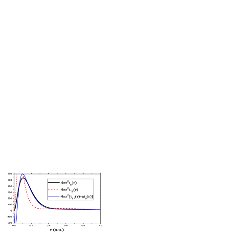
Figure 1: Radial TF kinetic energy densities for the neon atom.

Figure 2: Radial GEA2 kinetic energy densities for the neon atom.

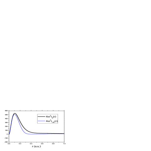
Figure 3: Radial vW kinetic energy densities for the neon atom.

Being $t_{S}^{I}(\mathbf{r})$ always positive, we choose it for convenience as the reference KED, whereas the corrections with the laplacians of the density are included as “laplacian contributions” to the approximated functionals. This can be done because comparing $t_{S}^{L}(\mathbf{r})=t_{S}^{I}(\mathbf{r})+at_{0}(\mathbf{r})$ with $t_{S}^{func}(\mathbf{r})$ is equivalent to compare $t_{S}^{func}(\mathbf{r})-at_{0}(\mathbf{r})$ with $t_{S}^{I}(\mathbf{r})$. We use $t_{S}^{I}(\mathbf{r})$, always positive, because it shows more clearly the KED in different regions of the space. Specifically, the figures exhibit a clear first shell and a small shoulder at the second shell (these features are verified against the radial density, $4\pi r^{2}n(r)$, and do not appear at the same positions when using $t_{S}^{II}(\mathbf{r})$).

For the TF functional (Fig. 1) we see that, without the laplacian contribution, the KED distribution has its main contribution to the kinetic energy in a region nearer to the nuclei than $t_{S}^{I}(\mathbf{r})$ has. The approximate KED with the laplacian contribution yields a more similar distribution but two eye-catching pathologies are shown. The peak corresponding to the $1s$ shell is exaggerated and a defect of KED is found near the nucleus. Instead, the asymptotic behavior seems to be almost correct.

For GEA2 we can observe (Fig. 2) qualitatively almost the same behavior than the TF, but now the pathologies are bigger. It is now clear how this gradient correction yields better values of the total kinetic energy than TF, without improving the local behavior of the KED, being the differences with the reference distribution bigger and the value of $\sigma$ worse.

For the von Weizsäcker functional (Fig. 3) very different results are obtained. The approximated KED is always smaller than the exact one, reflecting that when the von Weizsäcker functional is written in the form given by the equation (8), it is a local lower bound for the first definition of the KED. That is, the vW functional is not only a lower bound to the total kinetic energy but is also a local lower bound for the KED,Hoffman-Ostenhof and Hoffman-Ostenhof (2001) and there is no need for any laplacian correction. Note that in this case the contribution of the laplacian of the electron density yields a curve that is almost indistinguishable from the curve without it, as commented in section VII, and it is not depicted. It can be noted that $t_{vW}$ is only correct near the nucleus and in the asymptotic decay – the single orbital regions–, as expected from the definition of the vW functional.Yang et al. (1996)

IX Conclusions

We have developed a method to test kinetic energy density functionals attending not only to the total kinetic energies but looking at the local behavior of the kinetic energy densities associated to the functionals. To obtain quantitative measure of the accumulated difference between the distributions we have defined a quantity $\sigma$ that we have called quality factor. Due to the non-uniqueness of the KED definition we have performed comparisons with an infinite family of kinetic energy densities, $t_{S}^{L}(\mathbf{r})$, generated by adding to the definition of the orbital-based KED the laplacian of the electron density multiplied by a variable prefactor.

The procedure have been employed to test the local quality of twenty one semilocal functionals. We check the fitting of the KED corresponding to each functional to the closest $t_{S}^{L}(\mathbf{r})$ given by Eq. (17). For a given functional, we got values of $a$ (that weights the contribution of the laplacian), corresponding to a minimum value of $\sigma$, that show a small dependence on the atomic number $Z$. And for that value of $a$ the corresponding KED is always closer to the mean of the first and second definitions of the orbital-based KED than to the definitions themselves. This result recalls that this mean has been proved to be the more natural definition for a “classical” KED.Lombard et al. (1991); Yang et al. (1996)

The main result found is the unexpected failure of all semilocal functionals but those with a full vW term to improve the local pathologies of the Thomas-Fermi functional. Our measurement technique assures that, even the GGA corrections to the TF functional always yield better total kinetic energies, this semilocal functionals get worse local KEDs. This result confirms the preliminar calculations presented in Ref. García-Aldea and Alvarellos, 2005. The only exception to this rule is the Pearson functional, that yields bad values for the total kinetic energies.

Finally, we have qualitatively studied the behavior of the KEDs, showing the characteristic pathologies of the TF functional, that exhibits an excess in the first peak of the density (corresponding to the $1s$ orbital) and a defect near the nucleus. This pathologies are always enlarged in all the semilocal functionals, reflecting the main conclusion of this paper.

—————————————————– —————————————————–