Superfluid-Insulator and Roughening Transitions in Domain Walls

Abstract

We have performed quantum Monte Carlo simulations to investigate the superfluid behavior of one- and two-dimensional interfaces separating checkerboard solid domains. The system is described by the hard-core Bose-Hubbard Hamiltonian with nearest-neighbor interaction. In accordance with Ref. Burovski , we find that (i) the interface remains superfluid in a wide range of interaction strength before it undergoes a superfluid-insulator transition; (ii) in one dimension, the transition is of the Kosterlitz-Thouless type and is accompanied by the roughening transition, driven by proliferation of charge-$1/2$ quasiparticles; (iii) in two dimensions, the transition belongs to the 3D $U\left(1\right)$ universality class and the interface remains smooth. Similar phenomena are expected for domain walls in quantum antiferromagnets.

I Introduction

Strongly correlated quantum lattice systems represent one of the most exciting and active fields in condensed matter physics. On the fundamental physics side, they provide a rich playground to investigate quantum phase transitions and study new exotic states of matter (for a review see e.g. Bloch and as an example of more exotic systems see e.g. exotic_1 ; exotic_2 ). On the experimental side, the possibility of trapping bosons in optical lattices in a highly controllable manner makes such systems good candidates for applications in a variety of different fields such as quantum communication, computing, and precision measurements Jaksch ; Duningham ; Rodriguez . In particular, recently there has been a great interest toward studying trapped cold polar molecules for which the possibility of controlling long-range dipole-dipole interactions opens up the way to realization of novel quantum phases and possible use of this system for above mentioned applications (see polar_molecules1 and references therein).

Studies of quantum phases and transitions between them are mostly confined to well defined geometries and lattice types in a given dimension. It is, however, important to recognize that low-dimensional quantum systems can also emerge in the form of extended defects in a higher dimensional regular structure. Domain walls, grain boundaries and dislocations are the most prominent examples of such systems. Recently, stimulated by the observation of non classical moment of inertia in solid He-4 NCMI , superfluid properties of defects in crystals were looked at in Refs. Burovski ; He-gb ; Screw disl. . In particular, it has been shown that it is possible to have lower dimensional superfluid phases emerging on topologically frustrated defects in solid ⁴He.
For the scope of this work we are particularly interested in the results of Ref. Burovski , where the authors studied universal properties of the superfluid-insulator (SF-I) transition in interfaces separating two checkerboard (CB) domains by simulating the classical (d+1)-dimensional bond-current model bond-current . Here we briefly summarize their results. It has been shown that the grain boundary remains superfluid in a large range of parameters before undergoing the SF-I transition. In one dimension, the transition is of the Kosterlitz-Thouless (KT) type. An argument explaining why one should expect a roughening transition to happen simultaneously to the SF-I transition has been given: both transitions are driven by proliferation of one and the same quasiparticle carrying charge $1/2$. In two dimensions, however, the interface remains smooth and the transition belongs to the 3D $U\left(1\right)$ universality class.
At the qualitative level, the model studied in Ref. Burovski works for all systems of the same universality class. However, it can not be used for making quantitative predictions regarding realistic quantum bosonic Hamiltonians. These predictions are one of the main goals of our paper. In addition, we present a direct evidence for the fact that topological excitations carry charge-$1/2$, and quantitatively discuss the connection between roughening and SF-I transitions.

We are interested in studying grain boundaries in the CB solid which may be created in the system of hard-core cold bosons taken across the SF-CB transition. A possible experimental realization is represented by cold polar molecules in an optical lattice. In the interesting experimental regime, interparticle distances are such that double occupancy is strongly suppressed (giving rise to hard core bosons), while the nearest-neighbor interaction can be tuned via external electric fields polar_molecules1 ; polar_molecules2 .
The hard-core extended Bose-Hubbard Hamiltonian reads:

$$H=-t\sum_{<ij>}\left(a^{{\dagger}}_{i}\,a_{j}+h.c.\right)+V\sum_{<ij>}n_{i}n_{j}-\sum_{i}\mu_{i}n_{i}\;,$$ (1)

where $a^{{\dagger}}_{i}(a_{i})$ is the bosonic creation (annihilation) operator, $t$ is the hopping matrix element, $V$ is the nearest neighbor repulsion, and $\mu$ is the chemical potential. On a simple cubic/square lattice the model (1) is equivalent to the spin-1/2 XXZ antiferromagnet with exchange couplings $|J_{x}|=|J_{y}|=2t$, $J_{z}=V$ and magnetic field $h=zV/2-\mu$, where $z$ is the number of nearest neighbors. This correspondence makes our work equally relevant for studies of domain walls in spin systems, especially in the limit of strong anisotropy (or small domain wall width when the continuous approximation breaks down). The zero magnetic field case, i.e. $\mu=zV/2$, corresponds, in bosonic language, to half-integer filling factor. At half filling, the ground state of model (1) features the SF and CB phases only. The SF phase, characterized by broken U(1) symmetry, corresponds to the easy-plane antiferromagnet with the order parameter $\Psi=S_{x}+iS_{y}$, while the CB order, characterized by broken $Z_{2}$ symmetry, corresponds to the easy-axis antiferromagnet with long-range correlations in $S_{z}$ (here $S_{x,y,z}$ describe components of the Néel vector). While at a generic filling factor the system undergoes phase separation into SF and CB phases ground_state_phase_1 ; ground_state_phase_2 , at half filling the SF-CB transition happens at a special higher-symmetry point, $V=2t$, where the Hamiltonian (1) features an O(3) symmetry. In the spin model it corresponds to the Heisenberg point. At the Heisenberg point the Néel vector lives on a sphere and can point in any direction; it simply rotates from equator to the pole when going from the SF to the CB phase giving rise to the discontinuous (in terms of order parameters) SF-CB transition.

In what follows we consider a system initially prepared with two large solid domains with $S_{z}=M$ and $S_{z}=-M$ respectively, separated by a domain wall. To achieve this we consider a system of size $L_{x}=N+1,L_{y}(=L_{z})=N$ where N is an even integer, with periodic boundary conditions (PBC). For the easy-axis Hamiltonian, this results in a frustrated CB where two atoms can avoid occupying nearest neighbor sites everywhere but in the domain wall layer. Our goal is to study properties of the resulting $(d-1)$-dimensional interface embedded in a $d$-dimensional solid using quantum Monte Carlo simulations. We focus on the case of zero magnetic field (half filling factor), i.e. the chemical potential is fixed to $\mu=zV/2$, and show that the interface remains SF (has gapless magnons, in magnetic language) well beyond the bulk SF-CB transition, for a wide range of $V/t$.

Another interesting question concerns the roughness of the interface (for a brief review of roughening transition see e.g. roughening ). To be specific, an interface (viewed on large scale as a membrane) is said to be smooth if its mean square relative displacement, see Eq. (5) below, is finite in the thermodynamic limit. On the contrary, if the latter diverges with the system size, an interface is said to be rough. In this work we present numerical results, taken across the SF-I transition, of the mean square relative displacement for several system sizes.

The paper is organized as follows. In Subsection II A we present results for the 1D interface and show that the superfluid and roughening transitions happen simultaneously. In Subsection II B we consider a 2D interface and calculate the critical point for the SF-I transition. We briefly summarize our results in the Conclusion.

II Results

Our simulations are based on the Worm algorithm path integral approach worm algorithm , which allows efficient sampling of the many-body path winding numbers $\left\langle W_{\alpha}^{2}\right\rangle$ in imaginary time and space directions. In the path integral representation winding numbers have a simple geometrical meaning: $W_{\tau}=N$ is the number of particles in the system, and $W_{x,y,z}$ describe how many times the many-body trajectory loops around the system with periodic boundary conditions in directions $\hat{x}$, $\hat{y}$ or $\hat{z}$. Thus, winding number fluctuations in temporal and spatial directions define the compressibility and superfluid stiffness, respectively. Since we consider the easy-axis Hamiltonian at $V>2t$ and half integer filling, i.e. the system is in the insulating CB phase, the superfluidity is restricted to the plane of the grain boundary. As a consequence, we expect a nonzero value for spatial winding numbers only along directions parallel to the grain boundary. In the following we show that the superfluid response persists up to a critical value $(V/t)_{c}$, at which the interface undergoes the SF-I transition. In 1D interfaces this transition is of the Kosterlitz-Thouless type KT and is accompanied by roughening. In 2D the transition belongs to the 3D U(1) universality class and the interface remains smooth.
In order to calculate critical points (Fig. 2 and Fig. 7 below) we have performed simulations in a square system, i.e. $L_{\tau}\approx L_{y,z}=L$, where $L_{\tau}=c\beta$. Here $c=\sqrt{\rho_{s}/\kappa}$ is the sound velocity. In practice, for each system size we choose $\beta$ such that $\left\langle W_{\tau}^{2}\right\rangle\sim\left\langle W_{y,z}^{2}\right\rangle$. This requirement implies $c\approx L/\beta$, with the inverse temperature $\beta$ scaling with the system size. The last expression for $c$ comes from the dependence on winding numbers of the superfluid stiffness $\rho_{s}=\frac{L^{2-d}\langle\overrightarrow{W}^{2}\rangle}{\beta d}$, where $d$ is the system dimensionality and $\langle\overrightarrow{W}^{2}\rangle=\sum_{i=1,d}\;\langle{W_{i}^{2}}\rangle$, and compressibility $\kappa=\frac{\beta\langle{W_{\tau}^{2}}\rangle}{V}$, where $V$ is the volume.

II.1 One dimensional interface

Here we consider a system with $L_{x}=N+1$, $L_{y}=N$, which implies a grain boundary along the $\hat{y}$-direction. We start our study at $V/t=2.3$, slightly above the Heisenberg point $V/t=2$. We recall that winding number fluctuations in the superfluid phase are described by the gaussian distribution (see e.g. sf_density ), which in $d=1$ takes the form $P(W_{y}^{2})\propto\exp(-LW_{y}^{2}/2\beta\rho_{s})$. Similarly for winding numbers in imaginary time direction (particle number fluctuations) $P(W_{\tau}^{2})\propto\exp(-\beta W_{\tau}^{2}/2L\kappa)$. In $d=1$ the distributions are essentially discrete and the best way to extract superfluid stiffness and compressibility from the simulated distributions is by considering the following ratios:

$$\rho_{s}^{-1}=2\frac{\beta}{L}\ln\left[\frac{2P(W_{y}=0)}{P(W_{y}=-1)+P(W_{y}=+1)}\right],$$ (2)

and

$$\kappa^{-1}=2\frac{L}{\beta}\ln\left[\frac{2P(W_{\tau}=0)}{P(W_{\tau}=-1)+P(W_{\tau}=+1)}\right]\;.$$ (3)

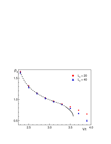
Figure 1: (Color online) Superfluid stiffness ($\rho_{s}$) vs interaction strength (V/t) for system sizes $L_{y}=20$ (circles) and $L_{y}=40$ (triangles) at zero temperature. The dashed line is to guide an eye, and the solid line represents $\rho_{s}$ in the thermodynamic limit, from finite size scaling. Error bars are within the symbol size.

We find that $W_{x}^{2}=0$ in our system sizes, ensuring that non-zero values for $W_{y}^{2}$ are due to grain boundary only. In Fig. 1 we plot the superfluid stiffness as a function of the interaction strength $V/t$, for system sizes $L_{y}=20$ (circles) and $L_{y}=40$ (triangles). The temperature has been chosen much smaller than the finite size energy gap, so that the system is effectively at zero temperature. The grain boundary remains superfluid, and, within statistical error bars, we do not see any size effects up to $V/t\gtrsim 3.5$. Finite-size effects indicate that we are approaching the SF-I transition in the interface.

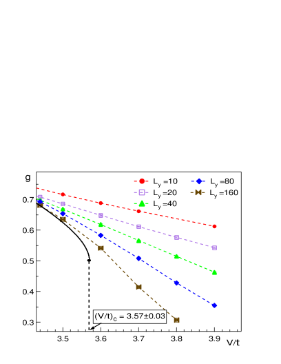
Figure 2: (Color online) Luttinger liquid parameter g as a function of $V/t$. (Error bars are within the symbol size). Dashed lines are to guide an eye; the solid line is the result of extrapolation to the infinite system size based on the Kosterlitz-Thouless theory. Simulation results are consistent with the universal jump at $g_{c}=0.5$. The critical value is at $(V/t)_{c}=3.57\pm 0.03$.

The 1D interface forms a Luttinger liquid and the quantum phase transition to the insulating state is of the Kosterlitz-Thouless type, characterized by the universal jump at $g=g_{c}=2/m^{2}$, where $g=\pi\sqrt{\rho_{s}\kappa}$ is the dimensionless Luttinger liquid parameter (see e.g. g-luttinger ) and $1/m$ is the fractional filling factor. In Fig. 2, we show $g$ as a function of $V/t$ for various system sizes (data are taken in square systems). Clearly, simulation results are fully consistent with the universal jump at $g_{c}=0.5$, which implies an effective filling factor $1/2$ in the grain boundary. The only logical explanation for fractional filling factor when translation symmetry in the bulk is broken with doubling of the unit cell volume, is to assume that the SF boundary is rough. Rough interface effectively averages the bulk potential and thus retains the original translation symmetry of the lattice. At the microscopic level, superfluidity and roughening are both linked to the proliferation of spinon excitations, and we provide additional evidence for this explanation below. In the figure, the solid line is the result of finite-size scaling based on the Kosterlitz-Thouless renormalization group (RG) flow KT . The integral form of the equations reads:

$$\int_{g(L_{1})/g_{c}}^{g(L_{2})/g_{c}}\dfrac{dt}{t^{2}(\ln(t)-\xi)+t}=4\ln(L_{1}/L_{2}),$$ (4)

where $\xi$ is a system size independent parameter. Using numerical data for $g(L)$ the integral can be solved numerically and $\xi(V/t)$ can be evaluated for each pair of sizes ($L_{1}$,$L_{2}$). In the critical region one expects $\xi$ to be a linear function of the interaction potential. At the critical point, Eq.(4) is satisfied by $\xi=1$.

In Fig. 3 we show the solution of Eq. (4) for three different pairs of ($L_{1}$,$L_{2}$). The data show a good collapse in the vicinity of the critical point $(V/t)_{c}=(3.57\pm 0.03)$. The $L\rightarrow\infty$ limit of Eq. (4) yields $(g(V/t)/g_{c})(\ln(g(V/t)/g_{c})-\xi(V/t))=-1$; its solution determines the thermodynamic value of the Luttinger liquid parameter $g$ indicated by the solid line in Figs. 2 and 1.

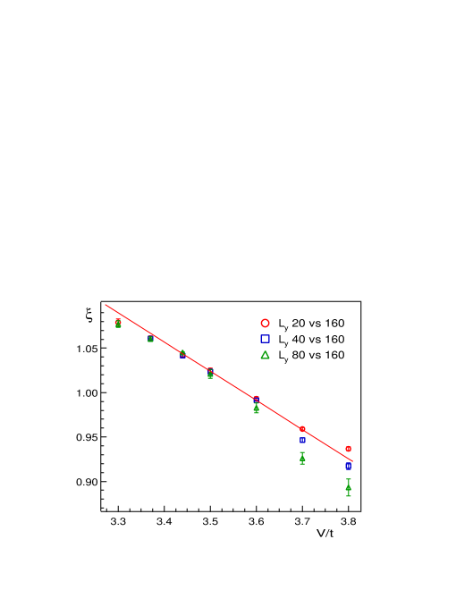
Figure 3: (Color online) Parameter $\xi$ for different pairs of system sizes $(L_{1},L_{2})$ as a function of (V/t). The solid line is a linear fit. The transition point is determined from the $\xi(V/t)=1$ condition.

We can explicitly verify that topological excitations driving the transition in 1D carry an effective charge of $1/2$. As it has been argued by Burovski et al., the propagation of kinks, or spinons, is achieved by shifting particles along the grain boundary. A single particle hopping event moves the grain boundary in the transverse direction and shifts the kink by two lattice steps. It means that in the presence of a gauge field a kink going around the system will accumulate half the gauge phase an ordinary particle will, i.e. its effective quasiparticle charge is 1/2.
In order to show that this is the case we measure how winding number fluctuations develop in imaginary time. The measurement is done for the insulating domain wall when winding number fluctuations are rare and one can study individual events. More specifically, we monitor $W_{y}^{2}$ and pick configurations with $W_{y}^{2}=1$. To suppress noise originating from quantum fluctuations in the solid bulk, we “filter” the trajectory by erasing hopping events which connect the same nearest neighbor sites and follow each other in imaginary time (see Fig. 4).

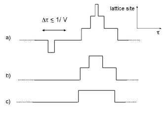
Figure 4: Here we show an example on how we “filter” the original trajectory a) by erasing hopping events, happening on a time scale $\Delta\tau\lesssim 1/V$, which connect the same nearest neighbor sites. Trajectories b) and c) show the result of ‘first and second filtering stage’ respectively. We stop the process at the second stage.

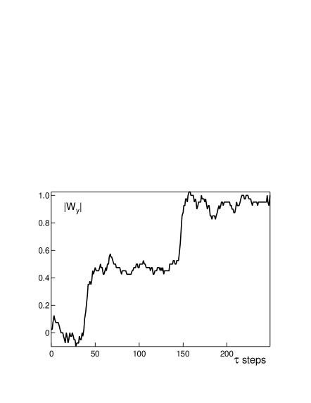
Figure 5: The development of the non-zero winding number along the grain boundary in imaginary time. The data refer to a system of size $L_{y}=20$ and $V/t=4.2$. The presence of steps implies that $W$ fluctuations happen in the form of instantons, i.e. the transition time from one ground state (degenerate in the thermodynamic limit) to another is a rare and fast virtual event. The step amplitude $\approx 1/2$ proves the fact that relevant elementary excitations carry charge $1/2$.

Figure 5 shows an example of the winding number trajectory for a system with $L=20$ and $V/t=4.2$. The first step describes system transition to an equivalent ground state obtained by shifting interface particles once, i.e. with the domain wall shifted by one unit length in the transverse direction. At this point the system has two choices: going back to the initial state or making another transition in the same direction and completing the full winding number (which has to be integer). This latter case is shown in Fig. 5 because we consider a configuration with $W_{y}^{2}=1$. As one moves closer to the transition point spinon excitations become more frequent and start overlapping in imaginary time making the whole picture less transparent for analysis.

Next we would like to discuss the connection between SF and roughening more quantitatively. In order to do so we have calculated the mean square displacement $\langle\Delta x^{2}\rangle$ of the grain boundary profile, where the average is done in both, imaginary time and space:

$$\left\langle\Delta x^{2}\right\rangle=\left\langle\int_{0}^{L_{y}}\int_{0}^{\beta}\Delta x^{2}(y,\tau)d\tau dy\right\rangle\;.$$ (5)

Here $\Delta x(y,\tau)$ is the instantaneous position of the center of the wall (recall that the interface is along the $y$ direction), calculated from the center of the grain boundary at $(\beta L_{y})^{-1}\int\int x(y,\tau)d\tau dy$. To determine $x(y,\tau)$, we calculate the difference between the “instantaneous” densities of two consecutive sites along the $x$ direction, $\delta n(i,\tau)=|n(i,\tau)-n(i+\hat{x},\tau)|$. Note that by “instantaneous” density, $n(i,\tau)$, we mean an average over some time interval $\Delta\tau$ such that $1/V\ll\Delta\tau\ll\beta$, in order to eliminate zero point fluctuations. Within the checkerboard solid, $\delta n(i,\tau)\approx 1$. In the grain boundary, instead, one can have consecutive sites either both occupied or empty (with a fractional value of $n(i,\tau)$ in the superfluid state of the boundary). Practically, for any given $y$, we start from the first lattice site and determine $x(y,\tau)$ from $\min(\delta n(i,\tau))$.

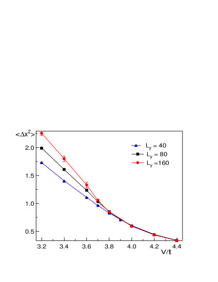
Figure 6: (Color online) The mean square displacement (measured in units of lattice spacing) of the grain boundary profile as a function of (V/t). In the insulating phase the data for different system sizes collapse, as expected for a smooth interface. Data start splitting in the vicinity of the critical point. In the superfluid state the interface is rough and $\langle\Delta x^{2}\rangle$ depends on the system size.

By definition, $\langle\Delta x^{2}\rangle$ is expected to be $\sim 1$ and system size independent for a smooth interface. For a rough interface, however, $\langle\Delta x^{2}\rangle$ diverges with the system size. Our results are consistent with this expectation as Fig. 6 shows. Beyond the transition to the insulating state, results for different system sizes overlap within statistical errors. On the superfluid side, instead, $\langle\Delta x^{2}\rangle$ increases with the system size $L$.

II.2 Two dimensional interface

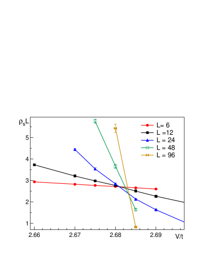
Figure 7: (Color online) Finite size scaling for the superfluid stiffness of a 2D interface. From the intersection of curves we estimate $(V/t)_{c}=2.683\pm 0.003$. Solid lines are to guide an eye.

Here we present results referring to a 3D system, i.e. 2D interface, at half integer filling factor. In this case the phase transition belongs to the $U(1)$ universality class in three dimensions, indicating a SF—Mott insulator transition at integer filling factor. As discussed in Ref. Burovski , the bulk acts as an effective periodic potential which doubles the primitive cell in the interface (if it remains smooth at the transition), bringing the filling factor from $1/2$ to $1$. In Fig. 7 we show the finite size scaling of the superfluid stiffness obtained from $\rho_{s}=\left\langle W^{2}_{y}+W^{2}_{z}\right\rangle/\beta$ (recall that the transverse direction is $x$), with $\beta$ scaling with the system size. From the intersection of scaled curves referring to different system sizes we obtain the critical point at $(V/t)_{c}=2.683\pm 0.003$.

In 3D, we did not observe quasiparticles carrying fractional charge $1/2$. Hopping of single particles along the interface remains a local fluctuation; to shift the wall one has to create a macroscopic line defect (“atomic step”) which is energetically expensive. Since the energy barrier between equivalent ground states increases with system size the interface remains smooth at $T=0$.

III Conclusions

To summarize, we studied superfluid-insulator transitions in 2D and 1D domain walls in the bosonic checker-board solid. In both cases domain walls remain superfluid well past the bulk SF-CB transition. In 1D the SF-I transition in the wall is intrinsically linked to the interface roughness since both properties are due to the proliferation of fractionally charged spinon excitations.

The minimal description of the system is given by the hard-core extended Bose-Hubbard Hamiltonian. Because on the bi-partite lattice the latter can be exactly mapped onto a spin 1/2 XXZ antiferromagnet model, the results presented here are also relevant to spin systems (for other lattice types the equivalent spin model is ferromagnetic in the xy-plane and antiferromagnetic along the z-axis). One can imagine creating domain walls in the system of ultra cold bosons in the process of fast ramping of the optical potential with several solid seeds nucleated at different locations in the trap. Clearly, the dynamics of grain boundaries and sample “annealing” will crucially depend on the the SF/roughening transitions. It might be also possible to observe signatures of lower-dimensional coherence in absorption images and interference experiments where none are expected for the ideal insulating bulk state.

The work was supported by the National Science Foundation under Grants PHY-0426881 and PHY-0653183.

References

- (1) E. Burovski, E. Kozik, A. Kuklov, N. Prokof’ev, and B.V. Svistunov, Phys. Rev. Lett. 94, 165301 (2005).
- (2) I. Bloch, J. Dalibard, W. Zwerger, cond-mat 0704.3011 (2007); I. Bloch, Nature Physics 1, 23 (2005).
- (3) F. Illuminati and A. Albus, Phys. Rev. Lett. 93, 090406 (2004); S. Ospelkaus, C. Ospelkaus, O. Wille, M. Succo, P. Ernst, K. Sengstock, and K. Bongs, Phys. Rev. Lett. 96, 180403 (2006).
- (4) A. D. Greentree, C. Tahan, J. H. Cole, and L. C. L. Hollenberg, Nature Physics 2, 856 (2006).
- (5) D. Jaksch and P. Zoller, Ann. Phys. 315, 52 (2005).
- (6) J.A. Dunningham and K. Burnett, Phys. Rev. A 70, 033601 (2004).
- (7) M. Rodriguez, S.R. Clark, and D. Jaksch, Phys. Rev. A 75, 011601(R) (2007).
- (8) A. Micheli, G. Pupillo, H.P. Büchler and P. Zoller, quant-ph/0703031.
- (9) E. Kim and M.H.W. Chan, Nature, 427, 225 (2004); Science 305, 1941, (2004).
- (10) L. Pollet, M. Boninsegni, A.B. Kuklov, N.V. Prokof’ev, B.V. Svistunov, and M. Troyer, Phys. Rev. Lett. 98, 135301 (2007).
- (11) M. Boninsegni, A.B. Kuklov, L. Pollet, N.V. Prokof’ev, B.V. Svistunov, and M. Troyer, cond-mat 0705.2976 (2007).
- (12) M. Wallin, E.S. Sørensen, S.M. Girvin, and A.P. Young, Phys. Rev. B 49, 12115 (1994).
- (13) H.P. Büchler, A. Micheli and P. Zoller, cond-mat/0703688.
- (14) F. Hébert, G.G. Batrouni, R.T. Scalettar, G. Schmid, M. Troyer, and A. Dorneich, Phys. Rev. B 65, 014513 (2001).
- (15) M. Kohno and M. Takahashi, Phys. Rev. B 56, 3212 (1997).
- (16) S. Balibar, H. Alles, A.Y. Parshin, Rev. Mod. Phys. 77, 317 (2005).
- (17) N.V. Prokof’ev, B.V. Svistunov, and I.S. Tupitsyn, Phys. Lett. A 238, 253 (1998); Sov. Phys. JETP 87, 310 (1998).
- (18) J.M. Kosterlitz and D.J. Thouless, J.Phys. C 6, 1181 (1973).
- (19) N.V. Prokof’ev and B.V. Svistunov, Phys. Rev. B 61, 11282 (2000).
- (20) V.A. Kashurnikov, A.I. Podlivaev, N.V. Prokof’ev, and B.V. Svistunov, Phys. Rev. B 53, 13091 (1996).