Dynamic structure factor of Fermi superfluid in the BEC-BCS crossover

Abstract

We consider cigar shaped Fermi superfluid in the BEC-BCS crossover. Using polytropic form of equation of state, we derive low energy multibranch bosonic excitations and the corresponding density fluctuations in three different regimes along the crossover, namely weak-coupling BCS, unitarity and molecular BEC regimes. Bragg spectroscopy can be used to probe the multibranch nature of the low energy bosonic excitations by measuring dynamic structure factor. Therefore, we calculate dynamic structure factor in those three different regimes. In the Bragg spectroscopy, an actual observable is momentum imparted to the superfluid due to the Bragg potential. We also present results of the momentum imparted to the superfluid due to the Bragg pulses.

I Introduction

The crossover from Bose-Einstein condensation (BEC) to Bardeen-Cooper-Schrieffer (BCS) state has drawn renewed interest in past few years due to rapid experimental progress in cold atomic two-component Fermi gases. Several experimental groups greiner ; jochim ; zw ; hara ; regal ; barten ; bourdel ; chin achieved the BEC-BCS crossover in the two-component atomic Fermi gases due to the magnetized Feshbach resonance mechanism houb ; stwa ; ties . The fermionic system becomes molecular BEC for strong repulsive interaction and transform into the BCS states when the interaction is attractive. Near the resonance, the zero energy $s$-wave scattering length $a$ exceeds the interparticle spacing and the interparticle interactions are unitarity limited and universal.

As in the case of bosonic clouds the frequencies of collective modes of Fermi gases can be measured to high accuracy. The collective oscillation frequencies of a trapped gas can provide crucial information on the equation of state of the system. The experimental results on the collective frequencies of the lowest axial and radial breathing modes on ultra cold gases of ⁶Li across the Feshbach resonance have also become available freq1 ; freq2 . Since the weak-coupling BCS and unitarity limits are characterized by the same collective oscillation frequency, it is an interesting to find out another observable which makes a clear identification of these two regimes and to better characterize two kinds of superfluid.

All the experiments of cold atomic Fermi gases are done in a cigar shaped geometry in which the atomic density is inhomogeneous in the radial plane and quasi-homogeneous along the symmetry axis. The axial excitations of a cigar shaped Fermi superfluid can be divided into two regimes: short wavelength excitations whose wavelength is much smaller than the axial size and long wavelength excitations whose wavelength is equal or larger than the axial size of the system. In the later case, the axial excitations are discrete and the lowest axial breathing mode frequency has been measured freq2 . In the former case, the short wavelength axial phonons with different number of radial modes of a cigar-shaped Fermi superfluid give rise to the multibranch spectrum zaremba . These are similar to the electromagnetic wave propagation in a wave guide. In the BCS side of the resonance, the low energy bosonic excitations, apart from the gaped fermionic excitations, of the Fermi superfluid are called multibranch Bogoliubov-Anderson (BA) modes. In the usual electronic superconductors, the BA phonon mode is absent due to the long-range Coulomb interaction.

In this work we find that the low energy multibranch modes in the BCS limit are different from that of in the unitarity limit, although discrete radial and axial mode frequencies are same due to the same exponent in the equation of state in the unitarity and BCS regimes. Therefore, these multibranch modes can be used to identify and characterize the weak-coupling BCS and unitarity states.

It is an interesting to study how one can probe such bosonic modes in the current available experimental setup. In fact, these multibranch low-energy bosonic modes could be observed by measuring dynamic structure factor (DSF) in a Bragg scattering experiment. Bragg spectroscopy of a trapped atomic system has proven to be an important tool for probing many bulk properties such as dynamic structure factor phonon , verification of multibranch Bogoliubov excitation spectrum in the usual atomic BEC mbs2 , correlation functions and momentum distributions of a phase fluctuating Bose gases ric ; gerbier . There has been a suggestion of Bragg scattering experiment to study the fermionic excitations at zero temperature deb as well as at temperature close to the critical temperature baym .

In this work, we also calculate DSF in the various regimes of the crossover, namely the weak-coupling BCS, unitarity and molecular BEC regimes. In actual Bragg scattering experiments, the measured response function is momentum transferred $P_{z}(t)$ to the superfluid by the Bragg pulses. The momentum transferred is directly related to the dynamic structure factor when time duration of the Bragg pulses is long enough. Therefore, we also study momentum transferred to the superfluid by the Bragg pulses. In order to probe the multibranch nature of the modes, we also estimate required values of wave vector and time duration of the two-photon Bragg pulses in the Bragg scattering experiments.

Recently, there is a measurement of sound velocity along the crossover sound . The measured sound velocity do not match with the theoretical prediction in the molecular BEC regime, however it matches very well in other regimes of the crossover tkgsound . One can also estimate the sound velocity in the three different regimes along the crossover by measuring slope of the phonon mode. It may resolve the puzzle of mismatch of the measured sound velocity with that of the theoretical prediction in the molecular BEC state.

This paper is organized as follows. In section II, we provide quantized hydrodynamic description of the Fermi superfluid along the crossover. In section III, we calculate the dynamic structure factor along the crossover. In section IV, we discuss the possible Bragg scattering experiment in this system and present results of the momentum transferred to the system due to the Bragg pulses. We also discuss a summary and conclusions in section V.

II quantized hydrodynamic theory of Fermi superfluid

We use hydrodynamic model with the Weizsacker quantum pressure term to describe low-energy dynamics of a two-component Fermi superfluid at zero temperature. This system can be well described by a time-dependent non-linear Schrodinger equation as follows kim :

$$i\hbar\frac{\partial\hat{\psi}({\bf r},t)}{\partial t}=[-\frac{\hbar^{2}}{2M}\nabla^{2}+V_{\rm ext}(r,z)+\bar{\mu}(n)]\hat{\psi}({\bf r},t),$$ (1)

where the non-linear term $\bar{\mu}(n)=\frac{\partial}{\partial n}[n\epsilon(n)]$ is the chemical potential in a uniform system and $\epsilon(n)$ is the ground state energy per particle. Here, $M$ is the mass of a Fermi atom and $V_{\rm ext}(r,z)=(M/2)(\omega_{r}^{2}r^{2}+\omega_{z}^{2}z^{2})$ is an external harmonic trap potential with $\omega_{r}>>\omega_{z}$. We have taken $\omega_{z}/\omega_{r}=0.1$ and total number of atoms $N=2.0\times 10^{6}$ in all numerical calculations. On the basis of quantum Monte Carlo data of Astrakharchik et al. astra , Manini and Salasnich manini proposed a very useful analytical fitting expression for $\epsilon(n)$ (see Eq. (6) and Table 1 of Ref. manini ). The Hamiltonian corresponds to Eq. (1) can be written as

$$H=\int d{\bf r}\hat{\psi}^{*}({\bf r},t)[-\frac{\hbar^{2}}{2M}\nabla^{2}+V_{\rm ext}(r,z)+\bar{\mu}(n)]\hat{\psi}({\bf r},t).$$

Using phase ($\theta$)-density ($n$) representation of the order parameter of the composite bosons: $\hat{\psi}({\bf r},t)=\sqrt{\hat{n}({\bf r},t)}e^{i\hat{\theta}({\bf r},t)}$, the above Hamiltonian becomes,

$$\hat{H} = \int d{\bf r}[\sqrt{\hat{n}}(-\frac{\hbar^{2}}{2M}\nabla^{2}\sqrt{\hat{n}})+\frac{1}{2}M{\hat{\bf v}}^{2}n+V_{\rm ext}(r,z)\hat{n}$$ (2)

$$+ \bar{\mu}(n)\hat{n}].$$

Linearizing the density and phase around their equilibrium values: $\hat{n}({\bf r},t)=n_{0}({\bf r})+\delta\hat{n}({\bf r},t)$ and ${\hat{\bf v}}({\bf r},t)=\delta{\hat{\bf v}}({\bf r},t)$, where ${\hat{\bf v}}=(\hbar/M)\nabla\hat{\theta}$ is the superfluid velocity. Keeping upto quadratic fluctuations, the above Hamiltonian reads

$$H=H_{0}+\int d{\bf r}[\frac{M\delta{\hat{\bf v}}^{2}}{2}+\frac{\partial\bar{\mu}}{\partial n}|_{n_{0}}\delta\hat{n}^{2}],$$ (3)

where $H_{0}$ is the ground state energy. By using time-dependent Heisenberg equations of motion for the density and velocity fluctuations, one can get continuity and Euler’s equations which are given by

$$\delta\dot{\hat{n}}=-\nabla\cdot[n_{0}(r)\delta\hat{\bf v}],$$ (4)

and

$$M\delta\dot{\hat{\bf v}}=-\nabla[\frac{\partial\bar{\mu}}{\partial n}|_{n_{0}}\hat{\delta}n].$$ (5)

Since the Hamiltonian is quadratic in terms of the fluctuation operators, it can be diagonalized by using the following standard canonical transformations:

$$\delta\hat{n}(r,z,t)=\sum_{j,k}[A_{j,k}\psi_{j,k}(r)\hat{\alpha}_{j,k}e^{i(kz-\omega_{j}(k)t)}+h.c.],$$ (6)

and

$$\delta\hat{\theta}(r,z,t)=\sum_{j,k}[B_{j,k}\psi_{j,k}(r)\hat{\alpha}_{j,k}e^{i(kz-\omega_{j}(k)t)}+h.c.].$$ (7)

Here, $j$ is a set of two quantum numbers: radial quantum number, $n_{r}$ and the angular quantum number, $m$. Also, $k$ is the axial wave vector. The density and phase fluctuations satisfy the following equal-time commutator relation: $[\delta\hat{n}(r),\delta\hat{\theta}(r^{\prime})]=i\delta(r-r^{\prime})$. One can easily show that

$$A_{j,k}=i\sqrt{\frac{\hbar\omega_{j}(k)}{2\frac{\partial\bar{\mu}}{\partial n}|_{n_{0}}}},B_{j,k}=\sqrt{\frac{2\frac{\partial\bar{\mu}}{\partial n}|_{n_{0}}}{\hbar\omega_{j}(k)}}$$ (8)

We are assuming that $\psi_{j,k}(r)$ satisfies the orthonormal conditions: $\int d{\bf r}\psi_{j,k}^{*}(r)\psi_{j^{\prime},k}(r)=\delta_{jj^{\prime}}$ and $\sum_{j}\psi_{j,k}(r)\psi_{j,k}^{*}({r}^{\prime})=\delta(r-r^{\prime})$.

We assume power-law form of the equation of state as $\bar{\mu}(n)=Cn^{\gamma}$. Here, $C$ depends on interaction strength and the effective polytropic index $\gamma$ is a function of a dimensionless parameter $y=1/k_{F}a$, where $k_{F}$ is the Fermi wave vector and $a$ is the scattering length between Fermi atoms of different components. The weak-coupling BCS ($y<<-1$) and the unitarity ($y=0$) states are described by the same exponent $\gamma=2/3$ with different values of $C$. For the weak-coupling BCS regime, $C_{\rm bcs}\simeq(3\pi^{2})^{2/3}(3\hbar^{2}/10M)$ and for the unitarity regime, $C_{\rm uni}=0.44C_{\rm bcs}$. The molecular BEC state ($y>>1$) is described by $\gamma=1$ and $C_{\rm bec}=4\pi\hbar^{2}a_{m}/M$, where $a_{m}=0.6a$ is the molecular scattering length gvs . In our calculation we have assumed $a_{m}=1.0\times 10^{-8}m$. The power-law form of the equation of state is being used successfully to study the Fermi superfluid along the crossover manini ; poly1 ; poly2 ; bulgac ; astra1 . At equilibrium, the density profile takes the form $n_{0}(r)=(\mu/C)^{1/\gamma}(1-\tilde{r}^{2})^{1/\gamma}$, where $\tilde{r}=r/R_{0}$, $R_{0}=\sqrt{2\mu/M\omega_{r}^{2}}$ and $\mu$ is the chemical potential in the non-uniform system, which can be obtained from the normalization condition.

Taking first-order time-derivative of Eq. (4) and using Eq. (5), the second-order equation of motion for the density fluctuation is given by

$$\frac{\partial^{2}\delta n}{\partial t^{2}}=\nabla\cdot[n_{0}(r)\nabla\frac{\partial\bar{\mu}(n)}{\partial n}|_{n=n_{0}}\delta n].$$ (9)

Using the polytropic form of the equation of state and Eq. (6), then Eq. (9) reduces to the following equation:

$$-\tilde{\omega}_{j}^{2}(k)\psi_{j,k}(r) = [\frac{\gamma}{2}\nabla_{\tilde{r}}\cdot[(1-\tilde{r}^{2})^{1/\gamma}\nabla_{\tilde{r}}(1-\tilde{r}^{2})^{1-1/\gamma}]$$ (10)

$$- \frac{\gamma}{2}\tilde{k}^{2}(1-\tilde{r}^{2})]\psi_{j,k}(r),$$

where $\tilde{\omega}=\omega/\omega_{r}$ and $\tilde{k}=kR_{0}$.

For $k=0$, it reduces to a two-dimensional eigenvalue problem and the solutions of it can be obtained analytically. The energy spectrum is given by

$$\tilde{\omega}_{j}^{2}=|m|+2n_{r}[\gamma(n_{r}+|m|)+1].$$ (11)

The corresponding orthogonal eigenfunction is given by

$$\psi_{j}\propto(1-\tilde{r}^{2})^{1/\gamma-1}\tilde{r}^{|m|}P_{n_{r}}^{(1/\gamma-1,|m|)}(2\tilde{r}^{2}-1)e^{im\phi},$$ (12)

where $P_{n}^{(a,b)}(x)$ is a Jacobi polynomial of order $n$ and $\phi$ is the polar angle.

The solution of Eq. (10) can be obtained for arbitrary value of $k$ by numerical diagonalization. For $k\neq 0$, we expand the density fluctuation as

$$\psi_{j,k}(r,\phi)=\sum_{j}b_{j}\psi_{j}(r,\phi).$$ (13)

Substituting the above expansion into Eq. (10), we obtain,

$$0 = [\tilde{\omega}_{j}(k)^{2}-[|m|+2n_{r}(\gamma(n_{r}+|m|)+1)]$$ (14)

$$- \frac{\gamma}{2}\tilde{k}^{2}]b_{j}+\frac{\gamma}{2}\tilde{k}^{2}\sum_{j^{\prime}}M_{jj^{\prime}}b_{j^{\prime}}.$$

Here, the matrix element $M_{jj^{\prime}}$ is given by

$$M_{jj^{\prime}}=\int d^{2}\tilde{r}\psi_{j}\tilde{r}^{2}\psi_{j^{\prime}}.$$ (15)

The above eigenvalue problem (Eq. (14)) is block diagonal with no overlap between the subspaces of different angular momentum, so that the solutions to Eq.(14) can be obtained separately in each angular momentum subspace. We can obtain all low energy multibranch spectrum on the both sides of the Feshbach resonance including the unitarity limit from Eq. (14). Equations (14) and (15) show that the spectrum depends on the average over the radial coordinate and the coupling between the axial mode and transverse modes within a given angular momentum symmetry. Particularly, the coupling is important for large values of $k$. We are interested to study $m=0$ states since these states are excited in the Bragg scattering experiments due to axial symmetry of the system. We show low energy multibranch modes of $m=0$ states in three different regimes in Fig. 1. The top three panels of Fig. 1 show the multibranch spectrum in the three different regimes. To compare these spectrum, we have plotted all those spectrum of different regimes in a single frame, which is shown in the bottom panel of Fig. 1. The lowest branch corresponds to the Bogoliubov axial mode with no radial nodes. This mode has the usual form $\omega=c_{s}k$ at low momenta, where $c_{s}$ is the sound velocity. In the limit of small $k$, the other branches have free-particle dispersion due to the gaped nature of these modes.

The discrete radial and axial modes are same in the unitarity and BCS regimes since the exponent $\gamma$ are the same for both the regimes. However, the multibranch modes are different in the unitarity and BCS regimes in spite of the same exponent in the equation of state. This is due to the different radial sizes in those two regimes for a given number of atoms and the trap potential. Therefore, these low energy axial propagation of discrete radial modes can be used to characterize different regimes of the superfluid. The density fluctuations for a fixed value of the axial momentum are plotted in Fig. 2. The density fluctuations corresponds to the multibranch modes are also different in the different regimes. In Fig. 2, the magnitude of the density fluctuations are given in an arbitrary unit since these are the linear fluctuations.

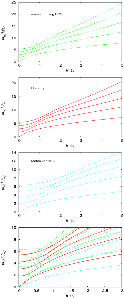
Figure 1: (Color online) Plots of the low energy multibranch modes in the three different regimes.

III dynamic structure factor

The dynamic structure factor is the Fourier transformation of density-density correlation functions and it is given as

$$S(k,\omega)=\int d{\bf r}d{\bf r}^{\prime}dt<\delta\hat{n}^{{\dagger}}({\bf r},t)\delta\hat{n}({\bf r}^{\prime},0)>e^{i{\bf k}\cdot({\bf r}-{\bf r}^{\prime})}e^{i\omega t}$$

This can be written as

$$S(k,\omega)=\sum_{j}S_{j}(k)\delta(\omega-\omega_{j}(k)),$$ (16)

where the weight factor $S_{j}(k)$ is given by

$$S_{j}(k)=\frac{\hbar\omega_{j}(k)}{2\frac{\partial\bar{\mu}}{\partial n}|_{n_{0}}}|\psi_{j}(k)|^{2}.$$ (17)

Here, $\psi_{j}(k)=\int d{\bf r}e^{-i{\bf k}\cdot{\bf r}}\psi_{j,k}({r})$ is the Fourier transform of the eigenfunctions $\psi_{j,k}({r})$. The weight factors are plotted in Fig. 3. The weight factors $S_{j}(k)$ determine how many modes are excited for a given value of $k$. For example, when $ka_{r}=1.0$, $n_{r}$ = {0, 1}, $n_{r}$ = {0, 1, 2 } and $n_{r}$ = {0, 1, 2, 3} modes are excited in the molecular BEC, unitarity and weak-coupling BCS regimes, respectively. The harmonic oscillator length is defined as $a_{r}=\sqrt{\hbar/M\omega_{r}}$. To excite many other low-energy modes, the wave vector in the Bragg potential must be large. From Fig. 3, it is clear that $S_{0}(k)\sim k$ and $S_{n_{r}>0}(k)$ is almost constant in the limit of small $k$. Therefore, $\omega_{0}(k)\sim k$ and $\omega_{n_{r}>0}(k)\sim k^{2}$ when $k$ is very small. Therefore, our analysis also satisfies the Feynman-like relation $\omega_{n_{r}}(k)\sim k^{2}/S_{n_{r}}(k)$. The dynamic structure factors of the three different regimes for $ka_{r}=0.5$ are plotted in Fig. 4. The delta function in Eq. (16) is replaced by the Lorentzian form to plot Fig. 4.

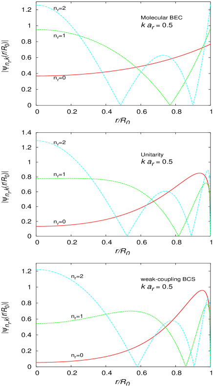
Figure 2: (Color online) Plots of the low-energy density fluctuations in the three different regimes for $ka_{r}=0.5$.

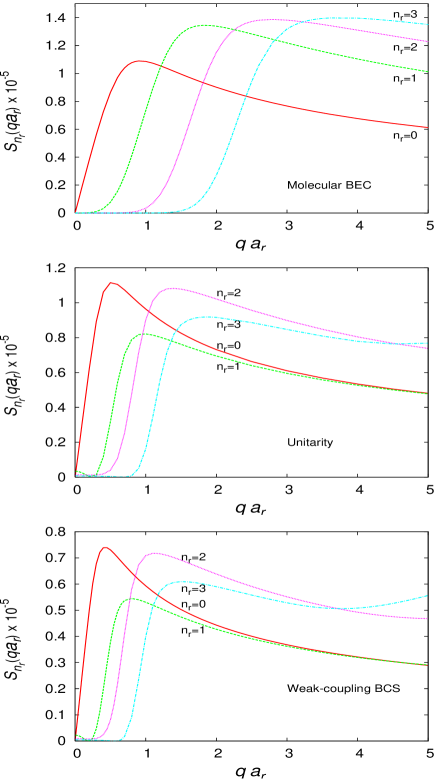
Figure 3: (Color online) Plots of the weight factors in the three different regimes.

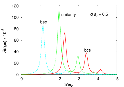
Figure 4: (Color online) Plots of the dynamic structure factors of the three different regimes for $ka_{r}=0.5$.

IV Bragg scattering experiment

The behavior of these multiple peaks in the dynamic structure factor can be resolved in a two-photon Bragg spectroscopy, as shown by Steinhauer et al. davidson for usual BEC. In the two-photon Bragg spectroscopy, the dynamic structure factor can not be measured directly. Actually, the observable in the Bragg scattering experiments is the momentum transferred to the superfluid, which is related to the dynamic structure factor and reflects the behavior of the quasiparticle energy spectrum. The populations in the quasiparticle states can be controlled by using the two-photon Bragg pulse. When the superfluid is irradiated by an external moving optical potential $V_{\rm op}=V_{B}(t)\cos(qz-\omega t)$, the excited states are populated by the quasiparticle with energy $\hbar\omega$ and the momentum $\hbar q$, depending on the value of $q$ and $\omega$ of the optical potential $V_{\rm op}$. Here, $V_{B}$ is the intensity of the Bragg pulse. Suppose the system is subjected to a time-dependent Bragg pulse which is switched on at time $t>0$ and $q$ is also along the $z$-direction. We calculate, similar to the calculation of Refs. tkg ; blak , the momentum transfer to the superfluid from the moving optical potential and it is given by

$$P_{z}(t) = \sum_{j,k}\hbar k<\hat{\alpha}_{j,k}^{{\dagger}}(t)\hat{\alpha}_{j,k}(t)>=\left(\frac{V_{B}(t)}{2\hbar}\right)^{2}$$ (18)

$$\times \sum_{j}\hbar qS_{j}(\tilde{q})\times[F_{j}(\omega_{-}t)-F_{j}(\omega_{+}t)],$$

where $\hat{\alpha}_{j,k}(t)$ is the time-evolution of the quasiparticle operator of energy $\hbar\omega_{j}(k)$ and

$$F_{j}(\omega_{\pm}t)=\left(\frac{\sin[(\omega_{j}(q)\pm\omega)t/2]}{(\omega_{j}(q)\pm\omega)/2}\right)^{2}.$$ (19)

For positive $\omega$ and a given $\tilde{q}$ such that $S_{j}(\tilde{q})$ is maximum, the momentum transferred $P_{z}(t)$ is resonant at the frequencies $\omega=\omega_{j}(q)$. The width of the each peak goes like $2\pi/t$. For large $t$ and $\omega_{z}<<\omega_{r}$, one can show that $P_{z}(t)\sim S(k,\omega)$ tozo .

In Fig. 5, we plot the net momentum transfer $P_{z}(t)$ vs the Bragg frequency $\omega$ for three different choices of the time duration of the Bragg pulses. Figure 5 shows that the shape of the $P_{z}(t)$ strongly depends on the time duration of the Bragg pulses $t_{B}$. When $t_{B}=0.5T_{r}$, $P_{z}(t)$ is a smooth curve with a single peak. Here, we define $T_{r}=2\pi/\omega_{r}$ is radial trapping period. When $t_{B}=1.0T_{r}$, there is a little evidence of few small peaks start developing in $P_{z}(t)$. When $t_{B}=2.0T_{r}$, the multiple peaks in $P_{z}(t)$ appears prominently. Therefore, the duration of the Bragg pulses $t_{B}$ should be greater than the radial trapping period $T_{r}$ in order to resolve different peaks in the DSF. Figure 5 also shows that the number of quasiparticle modes in unitarity regime is much higher than the other regimes of the crossover. This is due to the fact that $P_{z}(t)$ is proportional to the number of quasiparticle modes for a given $k$.

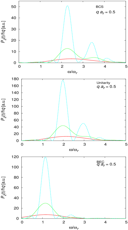
Figure 5: (Color online) Plots of the momentum transferred in the three different regimes for $ka_{r}=0.5$ and for different time duration of the Bragg pulses: $t=0.5T_{r}$ (solid), $t=1.0T_{r}$ (dashed) and $t=2.0T_{r}$ (dot-dashed).

V summary and conclusions

We have presented the quantized hydrodynamic theory of cigar shaped Fermi superfluid along the BEC-BCS crossover by using the power law form of the equation of state. We have calculated multibranch low energy bosonic modes and the corresponding density fluctuations in three different regimes along the BEC-BCS crossover, namely the weak-coupling BCS, unitarity and molecular BEC states. Then we have presented results of the dynamic structure factor calculation. We have also calculated the momentum transferred to the superfluid by the Bragg pulses and shown that the multibranch nature would be observed when the time duration of the Bragg pulses is greater than the radial trapping period.

We have found that the axial propagation of discrete radial modes in the weak-coupling BCS and unitarity regimes are different, although the axial and radial modes are same in both cases. One can identify these two regimes by probing these multibranch modes with the help of the Bragg scattering experiment. We have also seen that the number of quasi particle modes in the unitarity regime is quite large compared to other two regimes for a fixed value of the Bragg momentum and the number of atoms. Therefore, the response function in the unitarity regime will be more prominent than the other two regimes in the crossover. Moreover, one can estimate the sound velocities in different regimes along the crossover by measuring the slope of the phonon modes.

- (1) M. Greiner, C. A. Regal, and D. S. Jin, Nature 426, 537 (2003).
- (2) S. Jochim, M. Bartenstein, A. Altmeyer, G. Hendl, S. Riedl, C. Chin, J. H. Denschlag, and R. Grimm, Science 302, 2101 (2003).
- (3) M. W. Zwierlein, C. A. Stan, C. H. Schunck, S. M. F. Raupach, S. Gupta, Z. Hadzibabic, and W. Ketterle, Phys. Rev. Lett. 91, 250401 (1993).
- (4) C. A. Regal, M. Greiner, and D. S. Jin, Phys. Rev. Lett. 92, 040403 (2004).
- (5) M. Bartenstein, A. Altmeyer, S. Riedl, S. Jochim, C. Chin, J. H. Denschlag, and R. Grimm, Phys. Rev. Lett. 92, 120401 (2004).
- (6) T. Bourdel, L. Khaykovich, J. Cubizolles, J. Zhang, F. Chevy, M. Teichmann, L. Tarruell, S. J. J. M. F. Kokkelmans, and C. Salomon, Phys. Rev. Lett. 93, 050401 (2004).
- (7) C. Chin, M. Bartenstein, A. Altmeyer, S. Riedl, S. Jochim, J. H. Denschlag, and R. Grimm, Science 305, 1128 (2004).
- (8) K. M. O’Hara, S. L. Hemmer, M. E. Gehm, S. R. Grande, and J. E. Thomas, Science 298, 217 (2002).
- (9) M. Houbiers, H. T. C. Stoof, W. I. McAlexander, and R. G. Hulet, Phys. Rev. A 57, R1497 (1998).
- (10) W. C. Stwalley, Phys. Rev. Lett. 37, 1628 (1976).
- (11) E. Tiesinga, B. J. Verhaar, and H. T. C. Stoof, Phys. Rev. A 47, 4114 (1993).
- (12) J. Kinast, S. L. Hemmer, M. E. Gehm, A. Turlapov, and J. E. Thomas, Phys. Rev. Lett. 92, 150402 (2004).
- (13) M. Bartestein, A. Altmeyer, S. Riedl, S. Jochim, C. Chin, J. H. Denschlag, and R. Grimm, Phys. Rev. Lett. 92, 203201 (2004).
- (14) E. Zaremba, Phys. Rev. A 57, 518 (1998).
- (15) J. Stenger, S. Inouye, A. P. Chikkatur, D. M. Stamper-Kurn, D. E. Pritchard, and W. Ketterle, Phys. Rev. Lett. 82, 4569 (1999); D. M. Stamper-Kurn, A. P. Chikkatur, A. Gorlitz, S. Inouye, S. Gupta, D. E. Pritchard, and W. Ketterle, Phys. Rev. Lett. 83, 2876 (1999).
- (16) J. Steinhauer, N. Katz, R. Orezi, N. Davidson, C. Tozzo and F. Dalfovo, Phys. Rev. Lett. 90, 060404 (2003).
- (17) S. Richard, F. Gerbier, J. H. Thywissen, M. Hugbart, P. Bouyer, and A. Aspect, Phys. Rev. Lett. 91, 010405 (2003).
- (18) F. Gerbier, J. H. Thywissen, S. Richard, M. Hugbart, P. Bouyer, and A. Aspect, Phys. Rev. A 67, 051602 (2003).
- (19) B. Deb, J. Phys. B 39, 529 (2006).
- (20) G. M. Bruun and G. Baym, Phys. Rev. A 74, 033623 (2006).
- (21) J. Joseph, B. Clancy, L. Luo, J. Kinast, A. Turlapov, and J. E. Thomas, Phys. Rev. Lett. 98, 170401 (2007).
- (22) T. K. Ghosh and K. Machida, Phys. Rev. A 73, 013613 (2006).
- (23) Y. E. Kim and A. L. Zubarev, Phys. Rev. A 70, 033612 (2004).
- (24) G. E. Astrakharchik, J. Boronat, J. Casulleras, and S. Giorgini, Phys. Rev. Lett. 93, 200404 (2004).
- (25) N. Manini and L. Salasnich, Phys. Rev. A 71, 033625 (2005).
- (26) D. S. Petrov, C. Salomon, and G. V. Shlyapnikov, Phys. Rev. Lett. 93, 090404 (2004).
- (27) H. Heiselberg, Phys. Rev. Lett. 93, 040402 (2004).
- (28) H. Hu, A. Minguzzi, X. J. Liu, and M. P. Tosi, Phys. Rev. Lett. 93, 190403 (2004).
- (29) A. Bulgac and G. F. Bertsch, Phys. Rev. Lett. 94, 070401 (2005).
- (30) G. E. Astrakharchik, R. Combescot, X. Leyronas, and S. Stringari, Phys. Rev. Lett. 95, 030404 (2005).
- (31) J. Steinhauer, N. Katz, R. Ozeri, N. Davidson, C. Tozzo, and F. Dalfovo, Phys. Rev. Lett. 90, 060404 (2003).
- (32) T. K. Ghosh, Int. J. Mod. Phys. B 20, 5443 (2006).
- (33) P. B. Blakie, R. J. Ballagh, and C. W. Gardiner, Phys. Rev. A 65, 033602 (2002).
- (34) C. Tozzo and F. Dalfovo, New J. Phys. 5, 54 (2003).