Filtering of spin currents based on ballistic ring

Abstract

Quantum interference effects in rings provide suitable means for controlling spin at mesoscopic scales. Here we apply such a control mechanism to the spin-dependent transport in a ballistic quasi one dimensional ring patterned in two dimensional electron gases (2DEGs). The study is essentially based on the natural spin-orbit (SO) interactions, one arising from the laterally confining electric field ($\beta$ term) and the other due to to the quantum-well potential that confines electrons in the 2DEG ( conventional Rashba SO interaction or $\alpha$ term). We focus on single-channel transport and solve analytically the spin polarization of the current. As an important consequence of the presence of spin splitting, we find the occurrence of spin dependent current oscillations.

We analyze the transport in the presence of one non-magnetic obstacle in the ring. We demonstrate that a spin polarized current can be induced when an unpolarized charge current is injected in the ring, by focusing on the central role that the presence of the obstacle plays.

I Introduction

In recent years both experimental and theoretical physics communities have devoted a great deal of attention to the field of quantum electronics AAFKN98 . In particular a big effort has been devoted to the study and the realization of electric field controlled spin based devicesspintro . The main problem raised in this field is the generation of spin-polarized carriers and their appropriate manipulation. In order to realize a fully spin based circuitry, the interplay between spin-orbit (SO) coupling and quantum confinement in semiconductor heterostructures can provide a useful tool to manipulate the spin degree of freedom of electrons by coupling to their orbital motion, and vice versa.

Recently many works have been focusing on the so called spin Hall effect [3] ; [7] ; cul ; noish and most of the implementations in two dimensional electron gases (2DEGs) proposed for the spin manipulation are mainly based upon the SO interaction, which can be seen as the interaction of the electron spin with the magnetic field appearing in the rest frame of the electron. The SO Hamiltonian reads Thankappan

$$\hat{H}_{SO}=-\frac{\lambda_{0}^{2}}{\hbar}\;e{\bf E}({\bf r})\left[\hat{{\bf\sigma}}\times\left(\hat{\bf p}+\frac{e}{c}{\bf A}({\bf r})\right)\right].$$ (1)

Here ${\bf E}({\bf r})$ is the electric field, $\hat{{\sigma}}$ are the Pauli matrices, $\hat{\bf p}$ is the canonical momentum operator, ${\bf A}({\bf r})$ is a vector potential, ${\bf r}$ is a 3 dimensional position vector and $\lambda_{0}^{2}=\hbar^{2}/(2m_{0}c)^{2}$, where $m_{0}$ denotes the electron mass in vacuum. In materials $m_{0}$ and $\lambda_{0}$ are replaced by their effective values $m^{*}$ and $\lambda$.

In this paper we consider low dimensional electron systems formed by quasi-one-dimensional (Q1D) devices patterned in 2DEGs. In such systems there can be different types of natural SO interaction, such as: (i) the so-called Dresselhaus term which originates from the inversion asymmetry of the zinc-blende structure3t , (ii) the Rashba ($\alpha$-coupling) term due to the quantum-well potential Kelly that confines electrons to a 2D layer, and (iii) the confining ($\beta$-coupling) term arising from the in-plane electric potential that is applied to squeeze the 2DEG into a quasi-one-dimensional channel Thornton ; Kelly .

In this article we focus on the aspects of spin-interference in ballistic Q1D ring geometries with two leads subject to natural $\alpha$ and $\beta$-SO coupling. In fact coherent ring conductors enable one to exploit the distinct interference effects of electron spin and charge which arise in these doubly connected geometries. This opens up the area of spin-dependent Aharonov-Bohm physics, including topics such as Berry phases, B84 ; bphase spin-related conductance modulation,NMT99 ; MSC99 persistent currents, LGB90 ; SGZ03 spin filters PFR03 and detectors,ID03 spin rotation,MSC02 ; CMC03 and spin switching mechanisms FHR01 ; FHR03 ; HSFR03 .

In some earlier papers FRURIC the spin-induced modulation of unpolarized currents, as a function of the Rashba coupling strength, was discussed, often in the presence of an external magnetic field. In this paper we present a different mechanism based on the natural constant Rashba coupling, without the help of an external magnetic field. Here we also analyze the effects due to the $\beta$ coupling. As it was discussed in several papers noiq ; qse ; iii the in-plane electric potential, applied to patterned Q1D devices, can yield a high electric field in the plane of the 2DEG, leading to a sizeable $\beta$ term. In the above cited references, where this SO term was investigated by taking into account the sole confining potential, it was demonstrated that in some devices (such as a narrow Q1D wire) the effect of the $\beta$-SO term is analogous to the one of a uniform effective magnetic field, $B_{eff}$, orthogonal to the 2DEG ($x-y$ plane), and directed upward or downward according to the spin polarization along the $z$ direction.

The goals of the following treatment are: (a) checking the presence of the spin splitting in a Q1D ring due to the $\beta$ and (b) to the natural $\alpha$ SO coupling; (c) investigating quantum interference effects in rings; (d) analyzing the spin-induced modulation of unpolarized currents due to the SO term; (e) the discussion of the transport in the presence of a non-magnetic obstacle.

In order to pursue our aims we first analyze the $\beta$ coupling case, and then we discuss the apparently more difficult case of the $\alpha$ coupling.

In section II we discuss the analogies between the presence of a $\beta$-SO coupling and a transverse magnetic field in a Q1D narrow channel. Thus, we introduce the Hamiltonian for the Q1D ring, in order to calculate the eigenvalues and eigenstates and the spin splitting. In section III we present the ballistic approach to the transport through the ring and the quantum interference effects by analyzing the oscillations in the transmission. In section IV we discuss the possible spin-induced modulation of unpolarized currents also in the presence of a non-magnetic obstacle. In section V we extend our analysis to the $\alpha$ (Rashba) coupling by showing the analogies with the $\beta$ case. We demonstrate how the presence of a non-magnetic obstacle can produce a significant spin current by giving a novel mechanism for the ring based quantum spin filtering.

II $\beta$ SO coupling: model and relevant parameters

II.1 $\beta$-SO coupling and effective magnetic field

In this section we neglect the $\alpha$ (Rashba) coupling and the Dresselhaus term, so that the SO Hamiltonian in Eq.1 results very simplifiedmorozb

$$\hat{H}_{SO}^{\beta}=\frac{\lambda^{2}}{\hbar}\hat{\sigma_{z}}\left[{{\nabla V_{c}({\bf r})}}\times\left(\hat{\bf p}+\frac{e}{c}{\bf A}\right)\right]_{z}.$$ (2)

We can limit ourselves to the $z$ component, because the motion perpendicular to the 2DEG is quantum mechanically frozen out (i.e. with a mean value $\langle p_{z}\rangle=0$ in the ground state, for the potential well in the $z$ direction), while we assume that no external magnetic field is present so that ${\bf A}=0$. Notice that $S_{z}$ commutes with the Hamiltonian in Eq. 2, implying that the $\hat{z}$ component of the spin is preserved in the motion through the device. Thus the total Hamiltonian of an electron moving in a confining potential $V_{c}(r)$ is equivalent to that of a charged particle in a transverse magnetic field, but here the sign of ${B}_{eff}({\bf r})$ depends on the direction of the spin along $\hat{z}$noiq .

II.2 A Q1D channel

The basic brick of our device are narrow quantum wires (QWs), that are devices of width $W$ less than $1000\AA$thor and length up to some microns (here we think to a QW where $W\sim 5-100nm$). In these devices quantum effects are affecting transport properties. In fact, because of the confinement of conduction electrons in the transverse direction of the wire, their transverse energy is quantized into a series of discrete values. From a theoretical point of view a QW is usually defined by a parabolic confining potential along the transverse direction $\hat{x}$, with force $\omega_{d}$me i.e. $V_{c}(x)=\frac{m^{*}}{2}\omega_{d}^{2}x^{2}$.

In the special case of a QW $e{\bf\nabla}V_{c}({\bf r})\equiv m^{*}\omega_{d}^{2}(x,y,0)$ thus

$${B}_{eff}=\frac{\lambda^{2}}{\hbar}\;\frac{{m^{*}}^{2}\omega_{d}^{2}c}{e}\equiv\frac{\beta}{\hbar l_{\omega}}\frac{m^{*}c}{e},$$ (3)

where $l_{\omega}=\sqrt{\hbar/m^{*}\omega_{d}}$, while $\beta\equiv\lambda^{2}{m^{*}}\omega_{d}^{2}l_{\omega}$. Next, we introduce the effective cyclotron frequency $\omega_{c}=\frac{\beta}{\hbar l_{\omega}}$ ($\omega_{c}/\omega_{d}=\lambda^{2}/l_{\omega}$), the related frequency $\omega_{0}^{2}=\omega_{d}^{2}-\omega_{c}^{2}$ and the total frequency $\omega_{T}=\sqrt{\omega_{0}^{2}+\omega_{c}^{2}}$, thus

$$\hat{H}_{0}+\hat{H}^{\beta}_{SO}=\frac{\omega_{0}^{2}}{\omega_{T}^{2}}\frac{p_{y}^{2}}{2m^{*}}+\frac{p_{x}^{2}}{2m^{*}}+\frac{m^{*}\omega_{T}^{2}}{2}(x-x_{0})^{2},$$ (4)

where $x_{0}=s\frac{\omega_{c}p_{y}}{\omega_{T}^{2}m^{*}}$, $s=\pm 1$, corresponds to the spin polarization along the $z$ direction. Hence we can conclude that 4-split channels are present for a fixed Fermi energy, $\varepsilon_{F}$, corresponding to $\pm p_{y}$ and $s_{z}=\pm 1$. Notice the analogy with the Hamiltonian corresponding to one electron in the QW when an external transverse magnetic field is present.

II.3 The Q1D ring

Here we outline briefly the derivation of the Hamiltonian describing the motion of an electron in a realistic Q1D ringmeijer . We consider the 2DEG in the $xy$ plane; then we introduce a radial potential $V_{\text{c}}(r)$, so that the electrons are confined to move in a ring. The full single-electron Hamiltonian reads

$$H=\frac{{\bf p}^{2}}{2m^{*}}+V_{\text{c}}(r)+H^{\beta}_{\text{so}},$$ (5)

Due to the circular symmetry of the problem, it is natural to rewrite the Hamiltonian in polar coordinatesmeijer

$$H = -\frac{\hbar^{2}}{2m^{*}}\left[\frac{\partial^{2}}{\partial r^{2}}+\frac{1}{r}\frac{\partial}{\partial r}-\frac{1}{r^{2}}\left(i\frac{\partial}{\partial\varphi}\right)^{2}\right]+V_{\text{c}}(r)$$ (6)

$$+\frac{\lambda^{2}}{\hbar}e\frac{E_{r}(r)}{r}\left(-i\hbar\frac{\partial}{\partial\varphi}\right)\sigma_{z},$$

because the electric field has just the radial component. It follows that $L_{z}=-i\hbar\frac{\partial}{\partial\varphi}$ and $\sigma_{z}$ commute with the Hamiltonian $\hat{H}$ and the corresponding eigenvalues are $\pm\hbar\mu$ for $L_{z}$ and $\pm 1$ for $\sigma_{z}$.

In the case of a thin ring, i.e., when the radius $R_{0}$ of the ring is much larger than the radial width of the wave function, it is convenient to project the Hamiltonian on the eigenstates of

$$H_{0}=-\frac{\hbar^{2}}{2m^{*}}\left[\frac{\partial^{2}}{\partial r^{2}}+\frac{1}{r}\frac{\partial}{\partial r}\right]+V_{\text{c}}(r).$$

To be specific, we use a parabolic radial confining potential

$$V_{\text{c}}(r)=\frac{1}{2}m^{*}{\omega_{d}^{2}}(r-R_{0})^{2}\quad,$$ (7)

for which the radial width of the wave function is given by $l_{\omega}$. In the following, we assume $l_{\omega}/R_{0}\ll 1$ and neglect contributions of order $l_{\omega}/R_{0}$ to $H_{0}$ and to the centrifugal term,

$$H_{c}\simeq-\frac{\hbar^{2}}{2m^{*}R_{0}^{2}}\;\frac{\partial^{2}}{\partial\varphi^{2}}=\hbar\omega_{R}\frac{\partial^{2}}{\partial\varphi^{2}}.$$

In this limit, $H_{0}$ reduces to

$$H_{0}=-\frac{\hbar^{2}}{2m^{*}}\left[\frac{\partial^{2}}{\partial r^{2}}\right]+\frac{1}{2}m^{*}{\omega_{d}^{2}}(r-R_{0})^{2}\quad.$$ (8)

After some tedious calculations (see appendix A) we are able to obtain the energy spectrum of $H_{0}=H_{c}=H_{SO}$ as

$$\varepsilon_{n,\mu,s}\sim\hbar\sqrt{\omega_{d}^{2}+2\omega_{c}\omega_{R}\mu s}(n+\frac{1}{2})+\hbar\omega_{R}\mu^{2}.$$ (9)

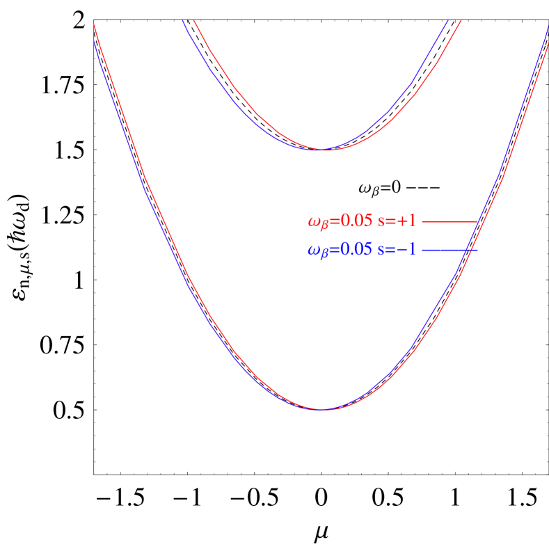
Figure 1: Bandstructure with and without the effects of the SO coupling. Notice the splitting: for each value of the Fermi energy $\varepsilon_{F}$ and for a fixed band $n$, there are 4 different eigenvalues. This spin dependent splitting in the energy allows for the interference phenomena that we next discuss.

The corresponding bandstructure is shown in Fig. 1. It follows that for fixed values of the Fermi energy, $\varepsilon_{F}$, and of the band $n$ there are 4 different eigenstates $\Psi_{n,\mu}^{s}$ i.e. particles with fixed Fermi energy $\varepsilon_{F}$ can go through the ring with four different wave numbers $\pm\mu_{\pm 1/2}$, depending on spin and direction of motion ($\pm$). Moreover the presence of non vanishing $\beta$ term implies an edge localization of the currents depending on the electron spins, also giving the presence of two localized spin currents with opposite chiralitiesnoish

Now we want to remark the presence of a spin splitting which is the basis of the interference phenomena in the transport through the ring. In the typical Aharonov-Bohm devices the phase difference is due to the enclosed flux of an external magnetic field. In the presence of a $\beta$ SO coupling the phase difference is generated by the splitting of the opposite spin polarized subbands.

In the presence of $\beta$ coupling the energy splitting is such that particles with Fermi energy $\varepsilon_{F}$ can go through the ring with four different wave numbers $\lambda\mu_{\lambda,s}$, depending on spin ($s$) and direction of motion ($\lambda=\pm$). The quantities $\lambda\mu_{\lambda,s}$ are obtained by solving $\varepsilon_{\mu,n}=\varepsilon_{F}$ and are not required to be integer. Because of the symmetry of the system, we can also obtain that $\mu_{+,\uparrow}=\mu_{-,\downarrow}$ and $\mu_{-,\uparrow}=\mu_{+,\downarrow}$. Next the fundamental quantity that we take in account is the phase difference $\pi\Delta\mu$, where

$$\Delta\mu=\mu_{+,\uparrow}-\mu_{-,\uparrow}=\mu_{-,\downarrow}-\mu_{+,\downarrow}\sim 2\frac{\omega_{c}}{\omega_{d}}.$$

III Theoretical approach to the transport through a ring

III.1 Ballistic transport and Landauer formula

We first consider the case where the 1D ring of Sec.II.b is symmetrically coupled to two contact leads (Fig.3.top panel left) in order to study the transport properties of the system subject to a constant, low bias voltage (linear regime). To this end, we calculate the zero temperature conductance $G$ based on the Landauer formula note9

$$G=\frac{e^{2}}{h}\sum_{n^{\prime},n=0}^{M}\sum_{\sigma^{\prime},\sigma}T_{n^{\prime}n}^{\sigma^{\prime}\sigma}\;,$$ (10)

where $T_{n^{\prime}n}^{\sigma^{\prime}\sigma}$ denotes the quantum probability of transmission between incoming ($n,\sigma$) and outgoing ($n^{\prime},\sigma^{\prime}$) asymptotic states defined on semi-infinite ballistic leads. The labels $n,n^{\prime}$ and $\sigma,\sigma^{\prime}$ refer to the corresponding mode and spin quantum numbers, respectively. In our case where $\sigma_{z}$ commutes with the Hamiltonian $T^{\uparrow\downarrow}=T^{\downarrow\uparrow}=0$. We also limit our analysis to the case of just one mode involved: $n=n^{\prime}=0$.

The Landauer formula works in the ballistic transport regime, in which scattering with impurities can be neglected and the dimensions of the sample are reduced below the mean free path of the electrons. Here we think to ring conductors smaller than the dephasing length $L_{\phi}$ i.e. with radius $R\lesssim 1\mu m$ for low temperatures ($T\ll 1^{o}K$). We also assume that this regime is not destroyed by the presence of just one obstacle as we will discuss below. We want also point out that the Landauer formula in the form of eq.(10) works just at $T=0$ while a more general formulation at finite temperatures has to take in account the width of the distribution of injected electrons.

III.2 Theoretical treatment of the scattering

We approach this scattering problem using the quantum waveguide theory2122 . For the strictly one dimensional ring the wavefunctions in different regions for each value of the spin are given below

$$\psi_{I} = e^{ikx_{1}}+r_{s}e^{-ikx_{1}}$$

$$\psi_{II} = A_{s}e^{i\mu_{+,s}\varphi}+B_{s}e^{-i\mu_{-,s}\varphi}$$

$$\psi_{III} = C_{s}e^{i\mu_{+,s}\varphi}+D_{s}e^{-i\mu_{-,s}\varphi}$$

$$\psi_{IV} = t_{s}e^{ikx_{2}},$$

where we can assume the wavevector of the incident propagating electrons in the leads $k\sim\mu/R_{0}$.

Thus we use the Griffith boundary condition23 , which states that the wave function is continuous and that the current density is conserved at each intersection. Thus we obtain the transmission coefficients.

III.3 Interference and oscillations in the transmission

Next we assume $\mu_{+,\uparrow}=\mu_{-,\downarrow}=\mu_{0}+\Delta\mu$ and $\mu_{+,\uparrow}=\mu_{-,\downarrow}=\mu_{0}-\Delta\mu$ with $\Delta\mu$ depending on the strength of the $\beta$ coupling.

Thus we obtain the transmission coefficient as we show in Fig.2,

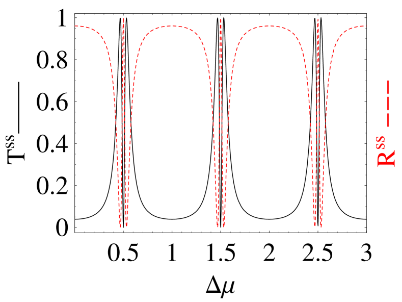
Figure 2: Oscillations in the transmission (and reflection) due to the difference of the phases of the waves with opposite chiralities. This is a quite general result that does not depend on the cause which gives the phase difference, $\Delta\mu$.

where the oscillations in the transmission are plotted as a function of the difference of phase, rescaled by factor $\pi$, i.e. $\Delta\mu$. Moreover it is clear that this kind of device is unable to produce a spin polarized current, because it results $T^{\uparrow\uparrow}=T^{\downarrow\downarrow}$.

The same result can be obtained by introducing a cut in the ring as an infinite barrier at $\varphi=\varphi_{B}$. In Fig.3 we show the oscillations in the transmission versus the position of the barrier.

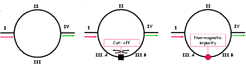
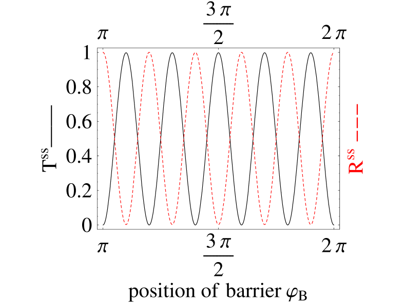
Figure 3: (Top)(Left) Schematic diagram of a ring connected to two leads. (Center) Schematic draw of the ring with a cut off in $\varphi_{B}=3\pi/2$ , i.e. interrupted by a totally reflecting barrier. On the right, the presence of a non magnetic obstacle. (Bottom) Oscillations in the transmission (and reflection) versus the cut position along the ring.

Also in this case, there is no way to select a spin polarized current, because it results $T^{\uparrow\uparrow}=T^{\downarrow\downarrow}$.

IV Modulation of spin unpolarized currents

Our main goal is to obtain a modulation of spin unpolarized currents. In order to do that, we need a symmetry breaking for the transport of opposite spin polarized current, i.e. $T^{\uparrow\uparrow}\neq T^{\downarrow\downarrow}$.

A central role, in order to pursue this goal, can be played by the presence of one or more obstacles along the path of the electrons along the ring. This is the case of impurities, disorder or restrictions in the channel’s width (e.g. due to the presence of a Quantum Point Contact along the channel). Next we analyze the presence of just one obstacle and we name it single non magnetic obstacle in analogy to the non magnetic impurity discussed in ref.[SGZ03, ].

IV.1 Effects of a non-magnetic obstacle

In order to discuss the effect of a non-magnetic obstacle on the transmission of the ring, we have to introduce a correction in our model. To simplify the problem, we will now assume that the obstacle is a delta-function barrier $V_{0}\delta(\varphi-\varphi_{B})$. Thus we can calculate the transmission by imposing the boundary conditions. Results are reported in Fig.4.

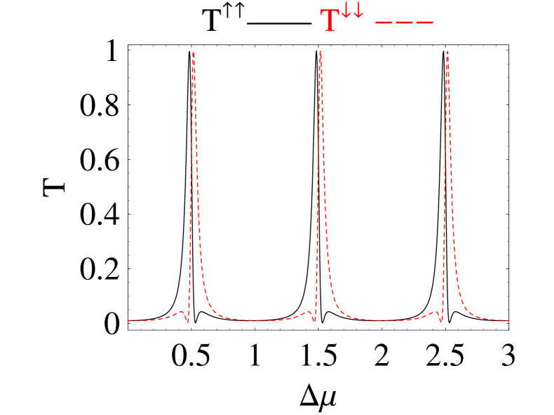
Figure 4: Transmission of the ring with a non magnetic obstacle at $\varphi_{B}=3\pi/2$. (Top) The spin transmissions versus the phase difference $\Delta\mu$. (Bottom) The extrapolated polarization, $P_{z}$ given in Eq. (11) of the emerging current.

In the presence of the obstacle the symmetry between the opposite spin polarization is broken and the transmission $T^{\uparrow\uparrow}$ differs from $T^{\downarrow\downarrow}$ (see Fig4.top). It follows that a spin polarized current can be observed at any values of $\Delta\mu$. Thus in the presence of just one obstacle the ring is able to select a polarized current.

From Fig.4 it is evident that the transmission polarized spin current is controlled by the phase difference, as well as by the modulation, analogously to the transmission charge current. In order to see this modulation clearly, we introduce a dimensionless quantity $P_{z}$ to describe the polarization along the $S_{z}$ spin axis of current transmitted through the Q1D ring, which is defined by

$$P_{z}=P_{z}(\pi\Delta\mu)=\frac{j_{\uparrow}-j_{\downarrow}}{j_{\uparrow}+j_{\downarrow}}=\frac{T^{\uparrow\uparrow}-T^{\downarrow\downarrow}}{T^{\uparrow\uparrow}+T^{\downarrow\downarrow}}.$$ (11)

Here the spin resolved currents $j_{s}$ were obtained employing the Landauer formula and $P_{z}$ turns out to be independent from the momentum of the incident charge carriers. This could yield an important advantage for device applications. Here $P_{z}$ is similar to the spin injection rate defined in ferromagnetic/semiconductor/ferromagnetic heterostructures233 , and it can be measured experimentallyapl .

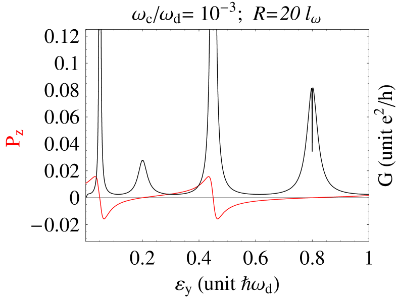
Figure 5: The spin polarization $P_{z}$ of the current exiting from a 1D ring (red line), an the charge conductance, as functions of the Fermi energy $\varepsilon_{F}$ for two realistic strength of the SO-$\beta$ coupling. We can observe that the presence of peaks in the spin polarization is related to dips in the charge transport. These dips in $G$ should correspond to the values of the Fermi energy which give integer angular momenta ($\mu=n$), but the presence of spin splitting doubles the peaks because of the symmetry breaking. We observe that the maximum spin polarization is obtained near the odd peaks.

V Modulation of spin current based on the Rashba SO coupling

V.1 $\alpha$-SO coupling

In what follows we take in account the natural $\alpha$ (Rashba) coupling Kelly . In semiconductors heterostructures, where a 2DEG is confined in a potential well along the $z$ direction, the SO interaction is of the type proposed by Rashba rashba : it arises from the asymmetry of the confining potential which occurs in the physical realization of the 2DEG, e.g. due to the band offset between $AlGaAs$ and $GaAs$. In this case the SO Hamiltonian in Eq.1 becomes

$$H_{\alpha}=\frac{\alpha}{\hbar}\left(\sigma_{x}\,p_{y}-\sigma_{y}\,p_{x}\right),$$ (12)

that in polar coordinates can be written as

$$H_{\alpha}=-\frac{\alpha}{r}\sigma_{r}\left(i\frac{\partial}{\partial{\varphi}}\right)+i\alpha\sigma_{\varphi}\frac{\partial}{\partial r}-\frac{i}{2}\frac{\alpha}{r}\sigma_{\varphi}.$$ (13)

Here $\sigma_{r}=\cos\varphi\,\sigma_{x}+\sin\varphi\,\sigma_{y}$ and $\sigma_{\varphi}=-\sin\varphi\,\sigma_{x}+\cos\varphi\,\sigma_{y}$. In the case of a thin ring, i.e. in the strictly one-dimensional case, when the radius $R$ of the ring is much larger than the radial width of the wave function $\l_{\omega}$, we can neglect the second term in the r.h.s. of Eq.13 and assume $r=R$, in agreement with the result in Eq. (2) of ref.(FRURIC, ).

As in the case of $\beta$ coupling we can introduce an effective magnetic field which in this case is oriented in the plane of the ring.

V.2 Energy bands and wavefunctions

After some tedious calculations we are able to obtain the energy spectrumFRURIC as

$$\varepsilon_{n,\mu,s} = \hbar\omega_{d}(n+\frac{1}{2})+\hbar\omega_{R}\left(\mu+\frac{1}{2}\right)^{2}+\frac{\hbar\omega_{R}}{4}$$ (14)

$$+ s{\hbar}\sqrt{\omega_{R}^{2}+\omega_{\alpha}^{2}}|\mu+\frac{1}{2}|,$$

where $\omega_{\alpha}=\alpha/(\hbar R)$ and $s$ is the spin polarization. If we introduce $j\equiv\mu+1/2$ eq.(14) becomes

$$\varepsilon_{0,j,s}=\frac{\hbar\omega_{d}}{2}+\hbar\omega_{R}\left(j-s\frac{j_{\alpha}}{2}\right)^{2}+\hbar\frac{\omega_{\alpha}^{2}}{\omega_{R}},$$ (15)

where $j_{\alpha}\equiv\sqrt{1+\frac{\omega_{\alpha}^{2}}{\omega_{R}^{2}}}$.

It follows that for a fixed value of the Fermi energy, $\varepsilon_{F}$, there are 4 different eigenstates $\Psi_{\pm,0,\mu}^{s}$ i.e. particles can go through the ring with four different wave numbers $\mu^{s}_{\pm,s}$, depending on spin ($s$) and direction of motion ($\pm$) as in the case discussed in the previous sections. The wave numbers can be obtained by solving the equation

$$\tilde{\varepsilon}=\hbar\omega_{R}(\mu+\frac{\Phi_{AC}^{\pm}}{2\pi})^{2},$$

where $\tilde{\varepsilon}\equiv\varepsilon_{F}-\hbar\omega_{d}/2-?\hbar{\omega_{\alpha}^{2}}/{\omega_{R}}$ and $\Phi_{AC}^{\pm}=-\pi(1\pm J_{\alpha})$ are the Aharonov Casher phase which are acquired while the two spin states evolve in the ring in the presence of the Rashba electric field.

The main difference with the $\beta$ case is that the spin are now polarized in a different direction i.e. $\hat{\bf s}_{\alpha}$ with an angle $2\theta$ respect to the $z$ axis corresponding to $\tan(2\theta)=\frac{\omega_{\alpha}}{\omega_{R}}$.

Thus that we can write the wavefunctions as

$$\Psi_{\pm,0,\mu}^{+} = u_{0}(r)e^{i\mu_{\pm,+}\varphi}\left(\begin{array}[]{c}\cos(\theta)\\ \sin(\theta)e^{i\varphi}\end{array}\right)\;\;\;$$ (18)

$$\Psi_{\pm,0,\mu}^{-} = u_{0}(r)e^{i\mu_{\pm,-}\varphi}\left(\begin{array}[]{c}\sin(\theta)\\ -\cos(\theta)e^{i\varphi}\end{array}\right)\;\;\;$$ (21)

Thus fundamental quantity which gives the phase difference is $\Delta\mu\pi$ is now given by $\Delta\mu=j_{\alpha}-1$.

V.3 From the transmission to the conductance

Now we can develop the calculations based on the Landauer formula in order to obtain the zero temperature conductance as discussed in section III. This approach, as we discussed above, is based on the calculation of the transmission amplitudes $T^{ss^{\prime}}=|t^{ss^{\prime}}|^{2}$. Thus we have to solve the scattering problem analogously to the case reported in section III by using the quantum waveguide theory.

Next we assume that the spin polarization along $\hat{\bf s}_{\alpha}$ is a constant of motion, thus $t^{+-}=t^{-+}=0$. Now we can write the coefficients $t$ in the two different basis as

$$t^{\uparrow\uparrow} = \cos^{2}({\theta})t^{++}+\sin^{2}({\theta})t^{--}$$

$$t^{\uparrow\downarrow} = -\cos({\theta})\sin({\theta})t^{++}+\cos({\theta})\sin({\theta})t^{--}$$

$$t^{\downarrow\downarrow} = -\sin^{2}({\theta})t^{++}-\cos^{2}({\theta})t^{--}$$

$$t^{\downarrow\uparrow} = \cos({\theta})\sin({\theta})t^{++}-\cos({\theta})\sin({\theta})t^{--}.$$ (22)

It follows that $t^{\uparrow\downarrow}=-t^{\downarrow\uparrow}$.

V.4 Modulation of a spin current

Our main goal is to obtain a modulation of spin unpolarized currents. In order to do that, we need a symmetry breaking for the transport of opposite spin polarized current, i.e. $T^{\uparrow\uparrow}\neq T^{\downarrow\downarrow}$ or $T^{\uparrow\downarrow}\neq T^{\uparrow\downarrow}$. The equations in Eq.(22) showed that if $t^{++}=t^{--}$ there is no symmetry breaking, in fact also $t^{\uparrow\downarrow}=-t^{\downarrow\uparrow}$. Thus as in the case of the $\beta$ coupling no spin polarization is present when we consider a clean ring.

A central role, in order to obtain a modulation of spin unpolarized currents, can be played by the presence of one or more obstacles along the path of the electrons in the ring as we discussed above. The corresponding symmetry breaking gives a significant spin polarization of the transmitted current

$$P_{z}=\frac{T^{\uparrow\uparrow}-T^{\downarrow\downarrow}}{T^{\uparrow\uparrow}+T^{\downarrow\downarrow}+2T^{\uparrow\downarrow}}.$$

It follows that a spin polarized current can be observed due to the Rashba phase shift (see Fig.7). Thus in the presence of just one obstacle the ring is able to select a polarized current. However by a comparison with the plots corresponding to the $\beta$ coupling it seems clear that a $\beta$-coupling based mechanism could be more efficient in obtaining a spin polarized current.

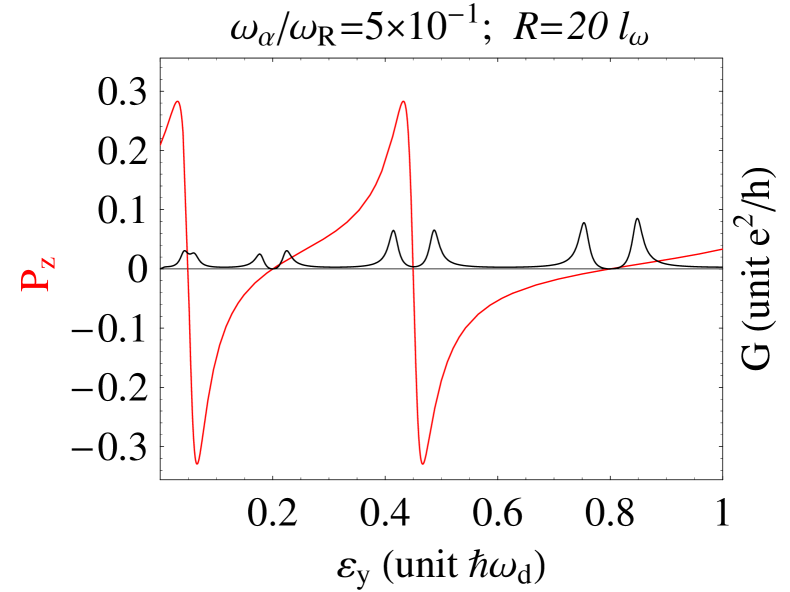
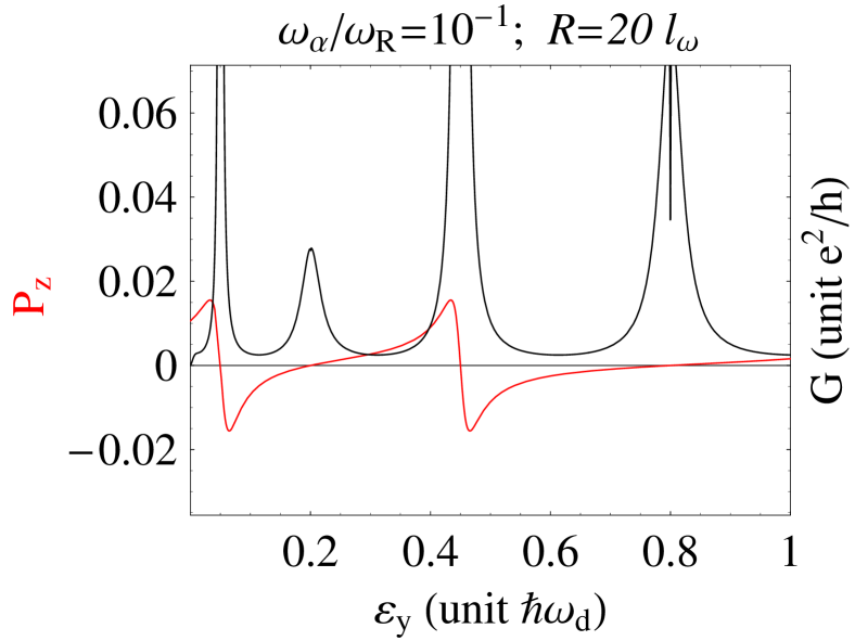
Figure 6: The spin polarization $P_{z}$ of the current exiting from a 1D ring (red line), an the charge conductance, as functions of the Fermi energy $\varepsilon_{F}$ for two realistic strength of the SO-$\alpha$ coupling. We can observe that the presence of peaks in the spin polarization is related to dips in the charge transport. These dips in $G$ should correspond to the values of the Fermi energy which give integer angular momenta ($\mu=n$), but the presence of spin splitting doubles some of the peaks, because of the symmetry breaking. However this splitting is clear just for strong values of the coupling. We observe that the spin polarization is significant near the odd peaks, whereas it vanishes in correspondence of the even peaks.

VI Discussion

The ring conductors have played an essential role in observing how coherent superpositions of quantum states (i.e., quantum-interference effects) on the mesoscopic scale leave imprints on measurable transport properties[26] . In fact they represent a solid state realization of a two-slit experiment, where an electron entering the ring can propagate in two possible directions (clockwise and counterclockwise). In these devices superpositions of quantum states are sensitive to the acquired topological phases in a magnetic [Aharonov-Bohm effect] or an electric [Aharonov-Casher effect for particles with spin] external field whose variations generate an oscillatory pattern of the ring conductance [27] .

In this paper we found that a non vanishing spin polarized current can be measured for a 2 leads ballistic ring in the presence of the natural $\alpha$ and $\beta$ term of the SO coupling. As we showed in Figs.5 and 6, some peaks in the spin polarization, $P_{z}$, are present near the measurable peaks in the charge conductance.All of our calculations are limited to the lowest subband but can be easily extended to the several subband case.

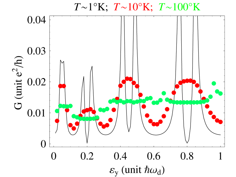
Figure 7: The charge conductance for three different scales of temperatures between $0K$ and some hundred degrees.

Moreover, in order to observe these oscillations at finite temperatures, the width of the distribution of injected electrons should not exceed the gap between the adjacent peaks of $G$ in Figs.5 and 6, while its center (i.e., $\varepsilon_{F}$ of the reservoirs) should be adjusted to their positionnprl . However for the spin-filter realization it is relevant to evaluate the efficiency of the device at non-zero temperature. Thus in the following we generalize our calculations at finite temperature $T$. The conductance at finite $T$ is given bycitro

$$G=-(e^{2}/h)\sum_{\sigma}\int_{0}^{\infty}d\varepsilon\frac{\partial f(\varepsilon,\varepsilon_{F},T)}{\partial\varepsilon}|T_{\sigma}(\varepsilon_{F})|^{2},$$ (23)

where $f$ is the Fermi distribution function and $T$ the temperature. As we show in Fig.7 the peaks disappear when the temperature becomes larger than some tens of $K$. Thus the proposed mechanism for the spin polarization works just at low temperatures.

In several papers (e.g. refs.(nprl, ; FRURIC, )) it was discussed how the tuning of the Rashba SO coupling in a semiconductor heterostructure hosting the ring generates quasiperiodic oscillations of the predicted spin-Hall current, due to spin-sensitive quantum-interference effects caused by the difference in the Aharonov-Casher phase accumulated by opposite spin states. In those cases an additional external field was needed in addition to the natural Rashba coupling. The authors of Refs.(nprl, ; FRURIC, )) proposed that the value of the $\alpha$ SOC could be tuned by controlling the transverse electric field by giving $\omega_{\alpha}/\omega_{R}$ in the range $0-10$. In the present work we discussed the transport in the presence of one non-magnetic obstacle in the ring with just the natural SO couplings, where the spin polarization of the current is governed by the gate voltage modulation. We demonstrated that a spin polarized current can be induced when an unpolarized charge current is injected in the ring thanks to the presence of the obstacle.

In section II and IV of this paper we assumed the $\alpha$-coupling to be negligible, although in general this term is comparable to (or larger than) the $\beta$-coupling term. By comparison with typical quantum-well and transverse electric fields, the SO-coupling constant $\beta$ can be roughly estimated as at least $\beta\sim 0.1\,\alpha$morozb . Moreover, in square quantum wells where the value of $\alpha$ is considerably diminished sw , the constant $\beta$ may well compete with $\alpha$. Furthermore the effects of the Rashba term on the spin polarization are often significant just for strong values of $\alpha$, some order of greatness larger than $\sim 10^{-11}\;eV\;m$(”natural” values of $\alpha$ at the GaAs interfaceNitta ) while the in plane $\beta$ coupling gives a good spin polarization in the currents also for small values of $\beta$, that are however larger than the usual ones (see ref.[noiq, ]).

It is clearly more difficult to modulate the strength of the $\beta$-SO coupling by acting on the split gate voltage. Thus the feasibility of a $\beta$ governed device mainly depends on its size and on the materials. The fundamental theoretical parameter in section IV, $\Delta\mu$, is proportional to the the ratio $\omega_{c}/\omega_{d}$, corresponding to $\lambda^{2}/l_{\omega}^{2}$, i.e. the ratio between a material dependent parameter $\lambda$ and a size dependent one $\l_{\omega}$ (that can be assumed to be a fraction of the real width,$W$, of the conducting channel). The SO strengths have been theoretically evaluated for some semiconductors compounds. In a QW ($W\sim 100$) patterned in InGaAs/InP heterostructures, where $\lambda^{2}$ takes values between $0.5$ and $1.5\,nm^{2}$, it results $\hbar\omega_{c}\sim 10^{-6}-10^{-4}eV$, corresponding to $\omega_{c}/\omega\sim 10^{-4}-10^{-3}$ as in InSb, where $\lambda^{2}\sim 500{\AA}^{2}$. For GaAs heterostructures, $\lambda^{2}$ is one order of magnitude smaller ($\sim 4.4{\AA}^{2}$) than in InGaAs/InP, whereas for HgTe based heterostructures it can be more than three times largerHgTe . However, the lithographical width of a wire defined in a 2DEG can be as small as $20nm$kunze ; thus we can realistically assume that $\omega_{c}/\omega_{d}$ runs from $1\times 10^{-6}$ to $1\times 10^{-1}$[notaf, ]. Here we can realistically assume that the ring has a width of just some tens of $nm$s.

The case reported in section V is more simple to be realized because in typical materials natural $\alpha$ is larger than $\beta$ and can also be tuned by controlling the transverse electric field. The phase shift is proportional to $\omega_{\alpha}/\omega_{R}$ so that a further modulation of the phase shift can be obtained by acting on the ring’s radius.

Thus, we can propose the discussed devices as spin filters based on the Q1D ring. We showed how the spin filtering is grounded on the presence of a non magnetic obstacle which produces a more or less spin polarized current. However, also in samples where spin polarization is quite smaller, the efficiency of a two leads ring as a spin filter can be amplified by realizing a series of these devices.

We acknowledge the support of the grant 2006 PRIN ”Sistemi Quantistici Macroscopici-Aspetti Fondamentali ed Applicazioni di strutture Josephson Non Convenzionali”.

Appendix A Spectrum and spin splitting

Next we can introduce the new variable $\xi=r-R_{0}$ ($p_{\xi}=-i\hbar\frac{\partial}{\partial r}$). The eigenvalues of $L_{z}$ are $\hbar\mu$ and the ones of $\sigma_{z}$ are $s$ ($S_{z}\equiv\frac{\hbar}{2}\sigma_{z}$). Thus we can write

$$H_{0}+H_{c}+H^{\beta}_{SO} \simeq \frac{p_{\xi}^{2}}{2m^{*}}+\frac{m^{*}}{2}\omega_{d}^{2}\xi^{2}+\frac{m^{*}}{2}\omega_{\beta}^{2}s\mu\xi^{2}$$ (24)

$$-\frac{m^{*}}{2}\omega_{\beta}^{2}s\mu 2R_{0}\xi+\hbar\omega_{R}\mu^{2},$$

where $\omega_{\beta}^{2}\equiv\frac{\beta}{m^{*}l_{\omega}R_{0}^{2}}$. Now we can introduce the new variables $\omega_{T}(\mu,s)^{2}\equiv\omega_{d}^{2}+\omega_{\beta}^{2}s\mu$ and $\xi_{0}(\mu,s)=\mu s\frac{\omega_{\beta}^{2}}{\omega_{T}(\mu,s)^{2}}R_{0}$, in order to obtain

$$H \simeq \frac{p_{\xi}^{2}}{2m^{*}}+\frac{m^{*}\omega_{T}(\mu,s)^{2}}{2}\left(\xi-\xi_{0}(\mu,s)\right)^{2}+\hbar\omega_{R}\mu^{2}$$

$$-\frac{m^{*}\omega_{\beta}^{4}R_{0}^{2}}{2\omega_{T}(\mu,s)^{2}},$$

from which the energy spectrum follows,

$$\varepsilon_{n,\mu,s}=\hbar\omega_{T}(\mu,s)(n+\frac{1}{2})+\hbar\omega_{R}\mu^{2}-\frac{m^{*}\omega_{\beta}^{4}R_{0}^{2}}{2\omega_{T}(\mu,s)^{2}}.$$ (25)

It follows that for fixed values of the Fermi energy, $\varepsilon_{F}$, and of the band $n$ there are 4 different eigenstates which have the general form

$$\Psi_{n,\mu}^{s}=u_{n}\left(r-R_{0}-\xi_{0}(s,\mu)\right)e^{i\mu\varphi}\chi_{s},$$

where $u_{n}(x)$ are the eigenstates of the 1D harmonic oscillator.

As we showed in ref.noish, the presence of non vanishing $\beta$ term implies an edge localization of the currents depending on the electron spins, also giving the presence of two localized spin currents with opposite chiralities. However, in our calculations we assume $u_{n}\left(\xi-\xi_{0}(s,\mu)\right)\simeq u_{n}\left(\xi+\xi_{0}(s,\mu)\right)$, in order to reduce the problem to a strictly one dimensional one.

References

- (1) Mesoscopic Physics and Electronics, T. Ando, Y. Arakawa, K. Furuya, S. Komiyama, and H. Nakashima, eds. (Springer, Berlin, 1998).
- (2) D. D. Awschalom, D. Loss, and N. Samarth, Semiconductor Spintronics and Quantum Computation (Springer, Berlin, 2002); B. E. Kane, Nature 393, 133 (1998).
- (3) M. I. D’yakonov and V. I. Perel’, JETP Lett. 13, 467 (1971).
- (4) J. Sinova, D. Culcer, Q. Niu, N. A. Sinitsyn, T. Jungwirth, and A. H. MacDonald, Phys. Rev. Lett. 92, 126603 (2004).
- (5) D. Culcer, J. Sinova, N. A. Sinitsyn, T. Jungwirth, A. H. MacDonald, and Q. Niu, Phys. Rev. Lett. 93, 046602 (2004).
- (6) S. Bellucci and P. Onorato, Phys. Rev. B 73, 045329 (2006).
- (7) L. D. Landau and E. M. Lifshitz, Quantum Mechanics (Pergamon Press, Oxford, 1991).
- (8) G. Dresselhaus, Phys. Rev. 100, 580 (1955).
- (9) M. J. Kelly Low-dimensional semiconductors: material, physics, technology, devices (Oxford University Press, Oxford, 1995).
- (10) T. J. Thornton, M. Pepper, H. Ahmed, D. Andrews, and G. J. Davies, Phys. Rev. Lett. 56, 1198 (1986).
- (11) M. V. Berry, Proc. R. Soc. London A 392, 45 (1984).
- (12) Several theoretical proposals LGB90 ; FHR01 ; FHR03 as well as experimental realizations[27] ; YPS02 exist.
- (13) D. Loss, P. Goldbart, and A. V. Balatsky, Phys. Rev. Lett 65, 1655 (1990).
- (14) D. Frustaglia, M. Hentschel, and K. Richter, Phys. Rev. Lett. 87, 256602 (2001).
- (15) D. Frustaglia, M. Hentschel, and K. Richter, Phys. Rev. B 69, 155327 (2004).
- (16) A.F. Morpurgo, J. P. Heida, T. M. Klapwijk, B. J. van Wees, and G. Borghs, Phys. Rev. Lett. 80, 1050 (1998).
- (17) J.-B. Yau, E. P. De Poortere, and M. Shayegan, Phys. Rev. Lett. 88, 146801 (2002).
- (18) J. Nitta, F. E. Meijer, and H. Takayanagi, Appl. Phys. Lett. 75, 695 (1999).
- (19) A. G. Mal’shukov, V. V. Shlyapin, and K. A. Chao, Phys. Rev. B 60, R2161 (1999).
- (20) J. Splettstoesser, M. Governale, and U. Zülicke, Phys. Rev. B. 68, 165341 (2003).
- (21) M. Popp, D. Frustaglia, and K. Richter, Nanotechnology 14, 347 (2003).
- (22) R. Ionicioiu and I. D’Amico, Phys. Rev. B 67, 041307(R) (2003).
- (23) A. G. Mal’shukov, V. Shlyapin, and K. A. Chao, Phys. Rev. B 66, 081311(R) (2002).
- (24) C. H. Chang, A. G. Mal’shukov, and K. A. Chao, cond-mat/0304508.
- (25) M. Hentschel, H. Schomerus, D. Frustaglia, and K. Richter, Phys. Rev. B 69, 155326 (2004).
- (26) S. Bellucci and P. Onorato, Phys. Rev. B74, 245314 (2006).
- (27) B. A. Bernevig and S. C. Zhang, Phys. Rev. Lett. 96, 106802 (2006).
- (28) Y. Jiang and L. Hu, Phys. Rev. B74, 075302 (2006).
- (29) D. Frustaglia and K. Richter, Phys. Rev. B 69, 235310 (2004).
- (30) A. V. Moroz and C. H. W. Barnes, Phys. Rev. B 61, R2464 (2000).
- (31) T. J. Thornton, Rep. Prog. Phys. 58, 311 (1995).
- (32) S. Bellucci and P. Onorato, Phys. Rev. B 68, 245322 (2003) and references therein.
- (33) F. E. Meijer, A. F. Morpurgo, and T. M. Klapwijk, Phys. Rev. B 66, 033107 (2002).
- (34) For a review see e.g. S. Datta, Electronic Transport in Mesoscopic Systems (Cambridge University Press, Cambridge, 1997).
- (35) J. B. Xia, Phys. Rev. B 45, 3593 (1992); P. S. Deo and A. M. Jayannavar, Phys. Rev. B 50, 11629 (1994).
- (36) S. Griffith, Trans. Faraday Soc., 49, 345 (1953); ibid. 49, 650 (1953).
- (37) M. Johnson, Phys. Rev. B 58, 9635 (1998); M. Johnson, and R. H. Silsbee, Phys. Rev. B 37, 5326 (1988).
- (38) Shen, Li, and Ma, Appl. Phys. Lett. 84, 996 (2004).
- (39) E. I. Rashba, Fiz. Tverd. Tela (Leningrad) 2, 1224 (1960), [Sov. Phys. Solid State 2, 1109 (1960)].
- (40) S. Washburn and R. A. Webb, Rep. Prog. Phys. 55, 1311 (1992).
- (41) S. Souma,B. K. Nikolic Phys. Rev. Lett. 94, 106602 (2005).
- (42) R. Citro, F. Romeo and M. Marinaro, Phys. Rev. B 74, 115329 (2006).
- (43) T. Hassenkam, S. Pedersen, K. Baklanov, A. Kristensen, C. B. Sorensen, P. E. Lindelof, F. G. Pikus, and G. E. Pikus, Phys. Rev. B 55, 9298 (1997).
- (44) J. Nitta, T. Akazaki, H. Takayanagi, and T. Enoki, Phys. Rev. Lett. 78, 1335 (1997).
- (45) X. C. Zhang, A. Pfeuffer-Jeschke, K. Ortner, V. Hock, H. Buhmann, C. R. Becker, and G. Landwehr, Phys. Rev. B 63, 245305 (2001).
- (46) M. Knop, M. Richter, R. Maßmann, U. Wieser, U. Kunze, D. Reuter, C. Riedesel and A. D. Wieck Semicond. Sci. Technol. 20, 814 (2005).
- (47) In any case should be larger than , so that at least one conduction mode is occupied.