Master crossover functions for the one-component fluid “subclass”

Abstract

Introducing three well-defined dimensionless numbers, we establish the link between the scale dilatation method able to estimate master (i.e. unique) singular behaviors of the one-component fluid “subclass” and the universal crossover functions recently estimated [Garrabos and Bervillier, Phys. Rev. E 74, 021113 (2006)] from the bounded results of the massive renormalization scheme applied to the $\Phi_{d}^{4}\left(n\right)$-model of scalar order parameter ($n=1$) and three dimensions ($d=3$), representative of the Ising-like universality class. The master (i.e. rescaled) crossover functions are then able to fit the singular behaviors of any one-component fluid without adjustable parameter, only using one critical energy scale factor, one critical length scale factor, and two dimensionless asymptotical scale factors, which characterize the fluid critical interaction cell at its liquid-gas critical point. An additional adjustable parameter accounts for quantum effects in light fluids at the critical temperature. The effective extension of the thermal field range along the critical isochore where the master crossover functions seems to be valid corresponds to a correlation length greater than three times the effective range of the microscopic short-range molecular interaction.

I Introduction

The universal features of three-dimensional (3D) Ising-like systems are now well-established by the renormalization group approach ZinnJustin2002 of the classical-to-critical crossover behavior Pelissetto2002 . In this theoretical context, it was possible to estimate the complete functions which interpolate between the critical behavior (controlled by the non-trivial (Wilson-Fisher) fixed point Wilson1972 ; Wilson1974 ) and a classical behavior (controlled by the Gaussian fixed point). Such interpolating theoretical expressions were customarily named classical-to-critical crossover functions. The corresponding crossover within the critical domain was referred as the critical crossover Pelissetto1998 ; Pelissetto2002 , or the asymptotic crossover Anisimov2000 .

Our present interest is restricted to the dimensionless expressions derived from a massive renormalization (MR) scheme applied to the $\Phi_{d}^{4}\left(n\right)$ model, for three-dimensional systems ($d=3$) and scalar order parameter ($n=1$) Bagnuls1984a ; Bagnuls1985 ; Bagnuls1987 ; Bagnuls2002 ($d$ and $n$ are the dimensions of the space and order parameter density, respectively, which characterize each universality class ZinnJustin2002 ). In that specific renormalization group approach MSRscheme , the Ising-like universality is linked to the existence of a unique non-trivial fixed point. For convenient simplification in the following presentation, the complete Ising-like universality class is labeled $\left\{\Phi_{3}\left(1\right)\right\}$-class (with reference to the $\Phi_{d=3}^{4}(n=1)$-model), while the one-component fluid “subclass” made of all one-component fluids is labeled $\left\{1f\right\}$-subclass, with the obvious relation $\left\{1f\right\}$-subclass $\subset\left\{\Phi_{3}\left(1\right)\right\}$-class.

The introduction of the system-dependent parameters for the practical use of the theoretical functions was discussed in a detailed manner in Refs. Bagnuls1984b ; Bagnuls1987 ; Bagnuls2002 ; Garrabos2006gb . More generally, the dimensionless forms of the theoretical expressions must be used to fit the experimental results in order to preserve both the number and the critical scaling nature of the fluid-dependent factors which are free in the massive renormalization scheme. Indeed, it was precisely shown in Ref. Garrabos2006gb , hereafter labeled I, that the Ising-like universal features Guida1998 , estimated in the Ising-like preasymptotic domain close to the non-trivial fixed point, require to characterize each system along its critical isochore (the thermodynamic line equivalent to $h=0$) using four parameters.

Two of them are dimensional parameters, namely the critical temperature $T_{c}$ which acts as energy unit (introducing the universal Boltzmann constant $k_{B}$) to express the Hamiltonian in dimensionless form, and the unknown inverse coupling constant $\left(g_{0}\right)^{-1}$ of the fourth-order term of the dimensionless Hamiltonian. As a matter of fact, any Hamiltonian representative of a physical system at near criticality, such as a one-component fluid near its liquid-vapor critical point, is driven to the non-trivial fixed point under the action of the renormalization transformations Wilson1974 . Due to the fact that renormalizable field theories are short-distance insensitive, universality emerges in a regime $\xi\Lambda_{0}\gg 1$ in which the correlation length $\xi$ is much larger than the microscopic scale, which plays the role of the inverse wavenumber cut-off $\left(\Lambda_{0}\right)^{-1}$ in the renormalization scheme. This universality is non-mean field like in nature (at least for the three-dimensional systems which are of present interest), because the actual molecular interaction range at the microscopic scale of the physical system cannot be completely eliminated. $\left(\Lambda_{0}\right)^{-1}$ remains the single natural length unit in the theoretical scheme. Indeed, $\left(g_{0}\right)^{-1}$ takes the convenient length dimension at $d=3$ to act as adjustable length unit, and to express the correlation length in dimensionless form.

The other two parameters are dimensionless coefficients, namely the scale factors $\vartheta$ and $\psi$, which provide the analytical (linear) proportionality between the two dimensionless physical fields $\Delta\tau^{*}$ and $\Delta h^{*}$ of the Ising-like fluid and the two renormalized relevant fields $t$ and $h$ of the $\Phi_{d=3}^{4}(n=1)$-model, respectively Wilson1972 ; Wilson1974 (using customarily field notations, see below). In such a situation, the universal features close to the non-trivial fixed point are estimated in conformity with the so-called two-scale-factor universality, where only two asymptotic critical exponents and one confluent exponent are independent. Then, the lowest value $\Delta\simeq 0.51$ Guida1998 of the confluent exponent characterizes the corrections to scaling due to one possible irrelevant field Wegner1972 ). In order to maintain the coherence with the previous presentation of these universal features given in Refs. Bagnuls2002 ; Garrabos2006gb , we have here also selected $\nu\simeq 0.630$ and $\gamma\simeq 1.240$ Guida1998 as independent leading exponents attached to the correlation length $\ell_{\text{th}}\left(t\right)$) and the susceptibily $\chi_{\text{th}}\left(t\right)$ along the critical isochore ($h=0$), respectively.

The finite scale $\left(\Lambda_{0}\right)^{-1}$ is generally unknown for a real microscopic interaction at short range distance in pure fluids. Simultaneously the macroscopic size $L$ of the fluid sample should be larger than $\xi$, i.e. $L\gg\xi\rightarrow\infty$, then a special attention to account for extensive nature of the thermodynamic properties of the physical system is needed. Moreover, thanks to the general point of view of the thermodynamics for 3-D systems, the dimensionless forms of any physical density variable $\frac{X}{V}$ (where $X$ is the total extensive variable and $V\propto L^{d}$ is the total volume of the system) can be obtained without reference to the unknown wavelength number $g_{0}$ defined at the critical point. Indeed, introducing the total amount of matter $N$ [or the total mass $M=Nm_{\bar{p}}$, where $m_{\bar{p}}$ is the mass of the particle, while the subcript $\bar{p}$ refers to a particle property] of a system filling a total volume $V$, the dimensionless order parameter conjugated to the dimensionless ordering field can always be defined if the amount of matter in a reference volume is known (here the reference volume can be chosen for example as the volume of a mole, a particle, a cell lattice, a mass unit of matter, etc.). Therefore, any reference length $a_{0}$, defined such as $n_{0}$ is the amount of matter in the volume $\left(a_{0}\right)^{d}$, can be used as explicit length unit for the thermodynamic and correlation functions. Thus the massive renormalization scheme generates a third adjustable dimensionless scale factor - namely $u_{0}^{*}=g_{0}a_{0}$ - which relates the dimensionless correlation length $\frac{\xi}{a_{0}}$ of the physical system to the corresponding theoretical function derived from the massive renormalization scheme. As a correlative result, when $a_{0}$ takes its physical sense to represent the effective range of the microscopic molecular interaction between the $n_{0}$ particles, i.e. $a_{0}\propto\left(\Lambda_{0}\right)^{-1}$ while $n_{0}\propto$ coordination number, the Ising-like singular nature of the physical system can be characterized by a set of three dimensionless scale factors $\left\{u_{0}^{*},\vartheta,\psi\right\}$. However, in such a three-parameter characterization of the physical system, it is then essential to recall that the theoretical estimations of the universal features are only valid within the Ising-like preasymptotic domain. In this preasymtotic domain, each dimensionless theoretical function can be approximated by its restricted asymptotic form as a two-term Wegner-like expansion, leading to three independent critical exponents (i. e. our selected set $\left\{\nu,\gamma,\Delta\right\}$ in present work).

Indeed, in the seventies, it was clearly shown by experimentalists that the singular properties of pure fluids close to their liquid-gas critical point were satisfied by power laws with universal features comparable to the ones estimated for the uniaxial three-dimensional Ising system used as a predictive model (for a review see for example Levelt1978 ). It was then revealed that two independent leading amplitudes, attached to the universal values of two independent critical exponents, are the only two fluid-dependent parameters necessary for characterizing the asymptotic singular behavior of each one-component fluid. Therefore, selecting the dimensionless correlation length $\xi^{*}\left(\Delta\tau^{*}\right)$ and the dimensionless isothermal compressibility $\kappa_{T}^{*}\left(\Delta\tau^{*}\right)$ in the homogeneous domain ($\Delta\tau^{*}>0$) along the critical isochore ($\Delta\rho^{*}=0$), each Ising-like critical fluid can then be characterized by the related leading amplitudes $\xi^{+}$ and $\Gamma^{+}$ (using standard notations for critical fluids Privman1991 ). This asymptotic situation characterized by two dimensionless leading amplitudes $\xi^{+}$ and $\Gamma^{+}$ was in conformity with the two-scale-factor universality expected for all systems, with short-ranged interaction, and which have an isolated transition point.

Correlatively, it was demonstrated Levelt1981 that the two-scale-factor universality related to the Ising-like nature of the critical phenomena in pure fluids are “observed” in a very limited range of temperature and densities around their liquid-gas critical point. Obviously, since the asymptotical critical domain associated to this limit is so narrow that experiments are difficult to achieve, it was fundamental to account for the possible nonuniversal character of the system through the confluent singularities in the corrections to scaling Wegner1972 (ignoring here the background contributions which are significative only in the case of specific heat Bagnuls1984b ). That leads to express the singular properties as truncated forms of the Wegner-like series. That precisely corresponds to the Ising-like limit of the asymptotic crossover mentionned just above and investigated in details in the renormalization theory where the resummation of the Wegner-like expansions should yield complete crossover functions from asymptotic (Ising-like) critical behavior to the classical (mean-field) critical behavior. Different theoretical approaches have been adopted by many investigators to obtain explicit solutions resumming the complete Wegner series (see for exemple a review in Ref. Anisimov2000 for their application to the fluid case). The practical results essentially depend on the approximations used in the renormalization scheme and the way to account for the cutoff effects. Despite these technical differences to treat the asymptotic crossover, the Ising-like universal feature was related to the lowest confluent exponent $\Delta$ where only one (fluid-dependent) confluent amplitude is needed to characterize the first order term of the confluent correction to scaling Wegner1972 . In the characterization of each critical fluid where the leading amplitudes $\xi^{+}$ and $\Gamma^{+}$ are selected in conformity with the asymptotic two-scale-factor universality, then it was necessary to add the confluent amplitude $a_{\chi}^{+}$ of the first order correction term for the susceptibility (related to the confluent amplitude $a_{\xi}^{+}$ of the correlation length by the universal value of the ratio $\frac{a_{\xi}^{+}}{a_{\chi}^{+}}\approx 0.68$ Guida1998 ). The resulting amplitude set $\left\{\xi^{+},\Gamma^{+},a_{\chi}^{+}\right\}$ defines the complete asymptotic crossover of each one-component fluid. This amplitude set is Ising-like equivalent (in quantity and nature) to the previous scale factor set $\left\{u_{0}^{*},\vartheta,\psi\right\}$ used to characterize the Ising-like critical behavior whitin the preasymptotic domain of each one-component fluid.

As recalled in I, this three-parameter description of the asymptotic singular behavior of the correlation length and the susceptibility of xenon was studied Bagnuls1984b using the crossover functions initially derived by Bagnuls and Bervillier Bagnuls1984a ; Bagnuls1985 from the massive renormalization scheme. In this pioneering study of the crossover, for the first time the minimal quantity of Ising-like non-universal parameters of xenon was introduced as a set of a single wavelength (defined at the critical point), and two dimensionless scale factors expressing the analytical approximation between the two relevant scaling (thermal-like $t$ and magnetic-like $h$) fields and the corresponding physical ($\Delta\tau^{*}$ and $\Delta h^{*}$) fields Wilson1972 ; Wilson1974 . Subsequently, theoretical and numerical approaches applied to the asymptotic crossover description of the singular behavior observed in pure fluids, have confirmed this characterization with three parameters (see for example Refs. Luijten1999 ; Luijten2000 ; Muser2002 ; Hahn2001 ; Zhong2003 ; Zhong2004 and a review in Ref. Anisimov2000 ).

Today, with the appropriate introduction of two fluid-dependent factors in conformity with the two-scale-factor universality, any theoretical function which fits the temperature dependence of the effective critical exponent along the critical isochore may be made universal by simply rescaling the temperature distance to the critical temperature, as initially proposed by Kouvel and Fisher Kouvel1964 who introduced a single crossover temperature scale $\Delta\tau_{X}^{*}$. Unfortunately, the unsolved problems in these theoretical approaches remain the validity of the linear approximations of two relevant fields (which correctly introduce the two system-dependent scale factors), the importance of the neglected analytical and non-analytical corrections, and, more generally, the estimation of the extension range in temperature and densities around the liquid gas critical point where the Ising-like universal features should be observed.

To complete the above introduction of the non-universal character of the asymptotic crossover in pure fluids, we also recall that, at the beginning of the eighties, the description of the behavior of the singular thermodynamic properties at finite distance from the liquid gas critical point was also made using the theoretical formulation of the nonasymptotic crossover from a regime of Ising-like scaled behavior to another regime in which the critical anomalies due to large fluctuations are ignored Chen1990b ; Chen1990a ; Anisimov1992 ; Anisimov1995 ; Anisimov2000 ; Agayan2001 . The common attempt to address this problem was based on the classical-to-critical crossover description of the free energy density. Indeed, this approach is useful for better understanding of crossover critical phenomena in “complex” fluids where the character of the crossover reflects an interplay between Ising-like universality caused by long-range fluctuations and a specific supramolecular structure characterized by an additional nanoscopic or mesoscopic length scale (which can then differ significantly from $\left(\Lambda_{0}\right)^{-1}$). Therefore, while the Ising-like two-scale-factor universality was similarly accounted for introducing the two dimensionless parameters of proportionality between the respective relevant (physical and renormalized) fields (for example $c_{t}\left(\sim\vartheta\right)$ and $c_{\rho}\left(\sim\psi\right)$ in the notations of Refs. Chen1990a ; Chen1990b ), the fundamental difference with the asymptotic crossover description comes from the introduction of two independent dimensionless parameters (for example $\bar{u}$ and $\Lambda$ in the notations of Ref. Anisimov1995 ), in order to control this nonasymptotic crossover character in complex fluids. However, in an application related to the pure fluid case, it is not necessary to introduce an additional mesoscopic length scale to account for the realistic microscopic situation in one-component fluids Hirschfelder1954 . Such pure fluids can then be assimilated to Lennard-Jones-like fluids when they are made of atoms or highly centro-symetrical molecules, or to short-distance associating fluids when they include more sophisticated short-range molecular interactions between unsymetrical molecules, polar molecules, bonding-like molecules, etc. Moreover, the representation of the experimental phase surface of any pure fluid by a van der Waals-like equation of state is not accurate either close or far away from the critical point (since the van der Waals equation of state is theoretically justified only for infinite range of the molecular interaction). As a final result, the fluid-dependent parameters needed to describe the classical behavior of the free energy density have no quantitative signification. The nonuniversal complexity of the pure fluid was then accounted for by introducing a significant number of adjustable parameters whose coupling with the two dimensionless crossover parameters $\bar{u}$ and $\Lambda$ can not be completely defined. Therefore, in spite of the correct introduction of a crossover function in the definition of variables and thermodynamic potentials, the only founded theoretical challenge of the nonasymptotic crossover applied to the one-component fluids remains to account for the correct Ising-like universal features with a single crossover scale. The uniqueness of the crossover scale can thus be defined introducing an arbitrary fixed value of the product $\bar{u}\Lambda$ Agayan2001 . The set $\left\{\bar{u}\left(or\,\Lambda\right),c_{t},c_{\rho}\right\}$ appears “Ising-like” equivalent to the set $\left\{u_{0}^{*},\vartheta,\psi\right\}$. This nonasymptotic crossover (which thus must match the asymptotic critical crossover close to the Wilson-Fisher fixed point Bagnuls1996 ) has to be not completely solved in regards to the most recent theoretical predictions of universal exponents Guida1998 ; Campostrini2002 and universal amplitude ratios Guida1998 ; Bagnuls2002 . Moreover, the introduction of the single crossover parameter, which is then related to the mean-field concept of the Ginzburg number Anisimov1992 , add conceptual difficulties to understand the role of real microscopic parameters controlling a true rescaled universal behavior in the whole crossover region Luijten1996 ; Pelissetto1998 ; Pelissetto2002 .

Finally, since the van der Waals dissertation, the real difficulty for scientists interested in liquid-gas critical phenomena in pure fluids, comes from the nonclassical (i.e. renormalizable) theories which are not able to predict the location of the critical point, while the classical theories provide its uncorrect location. Such a difficulty has generated a crucial experimental challenge where the determination of the two characteristic leading amplitudes and the characteristic crossover parameter of each pure fluid, and alternatively but equivalently, the localization of its liquid-gas critical point on the $p,V,T$ phase surface, remain mandatory.

Based on this recurrent situation, an alternative phenomenological way to characterize the asymptotic singular behavior of the one-component fluids was also formulated by Garrabos Garrabos1982 as follows: “If you are able to locate a single liquid gas critical point on the experimental $p,v_{\bar{p}},T$ phase surface of a fluid particle of mass $m_{\bar{p}}$, then you are also able to describe the asymptotic crossover around this isolated point”. $p$ is the pressure, $T$ is the temperature, $v_{\bar{p}}=\frac{V}{N}=\frac{m_{\bar{p}}}{\rho}$ is the volume of the particle, and $\rho$ is the (mass) density. Accordingly, a minimal set $Q_{c,a_{\bar{p}}}^{\text{min}}$ made of four critical coordinates Garrabos1982 [see below Eq. (1)], provides unequivocal determination of four (two dimensional and two dimensionless) scale factors [see below Eqs. (3) to (7)]. Then a scale dilatation method of the physical fields can be used to observe and quantify the master (i.e., unique) asymptotic crossover behavior of the $\left\{1f\right\}$-subclass Garrabos1985 ; Garrabos1986 . The two dimensional critical parameters, noted $\left(\beta_{c}\right)^{-1}$ and $\alpha_{c}$, take appropriate energy and length dimensions, respectively to reduce the physical variables, the thermodynamic functions, and the correlation functions. The two dimensionless critical numbers, noted $Y_{c}$ and $Z_{c}$, are well-defined characteristic parameters of the critical interaction cell of volume $\left(\alpha_{c}\right)^{d}$. An additional adjustable parameter, noted $\Lambda_{qe}^{*}$, accounts for quantum effects in light fluids at the critical temperature Garrabos2006qe . Conversely, when $Q_{c,a_{\bar{p}}}^{\text{min}}$ and $\Lambda_{qe}^{*}$ were known for the selected fluid, the asymptotic master behavior characterized by three master (i.e. constant) amplitudes was used to calculate the amplitude set $\left\{\xi^{+},\Gamma^{+},a_{\chi}^{+}\right\}$ which characterizes the asymptotic singular behavior of this fluid. In addition to this intrinsic predictive power, another important characteristic attached to the scale dilatation method was the Ising-like analogy in its formal introduction of the two dimensionless scale factors $Y_{c}$ and $Z_{c}$ and the corresponding ones $\vartheta$ and $\psi$ introduced by linear approximations in the massive renormalization scheme.

As a matter of fact, for each selected fluid belonging to the $\left\{1f\right\}$-subclass, this analogy can be useful to provide explicit estimation of the unknown scale factor set $\left\{\left(g_{0}\right)^{-1},\vartheta,\psi\right\}$ [or $\left\{u_{0}^{*},\vartheta,\psi\right\}$] of the theoretical crossover functions (using then, the thermodynamic length scale unit $\alpha_{c}$ of the selected one-component fluid as a reference length $a_{0}$). Especially in the case of the unique form of the mean theoretical functions estimated in I (which incorporates the error-bar propagation of the min and max crossover functions revisited in Bagnuls2002 ), we can formulate the unambiguous modifications of the theoretical crossover functions for the $\left\{\Phi_{3}\left(1\right)\right\}$-class to exactly match the master two-term Wegner-like expansions valid within the Ising-like preasymptotic domain of the $\left\{1f\right\}$ -subclass.

These formulations were used to study the correlation length in the homogeneous domain of seven one-component fluids Garrabos2006corlength and the squared capillary length in the non-homogeneous domain of twenty one-component fluids Garrabos2006sugden . Similarly, a recent application to the practical parachor correlations (i.e., equations expressing surface tension as a power law of the density difference between coexisting gas and liquid phases), have shown that the corresponding master form acts as a universal equation of state for the interfacial properties Garrabos2007pa . Now, our present objective is to achieve the complete uniquevocal link between these updated results of I and the scale dilatation method to predict the master singular behavior of the $\left\{1f\right\}$-subclass. For these studies, the analytical relations between the relevant scaling fields of both descriptions must be defined.

The paper is organized as follows. In Section 2 the master description of the universal features within the Ising-like preasymptotic domain is recalled. First, starting from the four critical coordinates of the critical point, we define four scale factors which are needed to unambiguously determine three dimensionless amplitudes which characterize the Ising-like preasymptotic domain of each one-component fluid. Second, we show the master singular behavior of the isothermal compressibility, applying the scale dilatation method to the related physical quantities. That complete the master sigular behavior of the correlation length in conformity with the two-scale-factor universality of the $\left\{\Phi_{3}\left(1\right)\right\}$-universality class. In Section 3, a brief presentation of the theoretical crossover functions for the correlation length and the susceptibility in the homogeneous phase is given to demonstrate the analytical matching with the master singular behavior provided by the scale dilatation method. Introducing three well-defined dimensionless numbers characterizing the $\left\{1f\right\}$-subclass, the unequivocal link between three theoretical amplitudes, which characterize the $\left\{\Phi_{3}\left(1\right)\right\}$-universality class, and three master amplitudes, which characterize the $\left\{1f\right\}$-subclass, is given before concluding in Section 4. Two appendices deal with first, the equivalence between different one-parameter crossover models, and second, the determination of the crossover parameter beyond the preasymptotic domain using the well-known linear model of the parametric equation of state with effective exponents.

II Master singular description of the one-component fluid subclass

II.1 The minimal set of critical parameters

For the $\left\{1f\right\}$-subclass, it was hypothesized Garrabos1982 Garrabos1985 that all the information needed to characterize non-quantum fluid critical phenomena is contained within the four critical parameters needed to localize the single critical point and its tangent plane on the experimental phase surface of normalized equation of state $\Phi_{a_{\bar{p}}}^{p}\left(p,v_{\bar{p}},T\right)=0$ (the needed supplementary information to characterize quantum fluids is given in Ref. Garrabos2006qe ; see also below Eqs. (9) and (10)). This minimal set of four coordinates reads as follows

$$Q_{c,a_{\bar{p}}}^{\text{min}}=\left\{T_{c},p_{c},v_{\overline{p},c},\gamma_{c}^{{}^{\prime}}\right\}$$ (1)

where $v_{\bar{p},c}=\frac{V}{N_{c}}=\frac{m_{\bar{p}}}{\rho_{c}}$ is the critical volume per particle ($V$ is the total volume, $N_{c}$ is the total critical number of particles, and $\rho_{c}$ is the critical density), and

$$\gamma_{c}^{{}^{\prime}}=\left(\frac{\partial p}{\partial T}\right)_{v_{\bar{p}}=v_{\bar{p},c};T=T_{c}}=\left(\frac{dp_{\text{sat}}}{dT}\right)_{T=T_{c}}$$ (2)

is the common critical direction of the critical isochore and the saturation pressure curve at the critical point, in the $p;T$ diagram. $\gamma_{c}^{{}^{\prime}}$ is related to the Riedel factor Riedel1954 , $\alpha_{R,c}=\left(\frac{d\log p_{\text{sat}}}{d\log T}\right)_{T=T_{c}}$, through the relation $\alpha_{R,c}=\frac{T_{c}}{p_{c}}\gamma_{c}^{{}^{\prime}}$. The subscript $c$ refers to a critical quantity. From Eq. (1), we can construct a more convenient set,

$$Q_{c}^{\text{min}}=\left\{\left(\beta_{c}\right)^{-1},\alpha_{c},Y_{c},Z_{c}\right\}$$ (3)

making use of the following four scale factors

$$\left(\beta_{c}\right)^{-1}=k_{B}T_{c}\sim\left[\text{energy}\right]\text{,}$$ (4)

$$\alpha_{c}=\left(\frac{k_{B}T_{c}}{p_{c}}\right)^{\frac{1}{d}}\sim\left[\text{length}\right],$$ (5)

$$Z_{c}=\frac{p_{c}v_{\overline{p},c}}{k_{B}T_{c}}\sim\left[\text{dimensionless}\right]\text{,}$$ (6)

$$Y_{c}=\left(\gamma_{c}^{{}^{\prime}}\frac{T_{c}}{P_{c}}\right)-1\sim\left[\text{dimensionless}\right]$$ (7)

$\left(\beta_{c}\right)^{-1}$ and $\alpha_{c}$ are used to express dimensionless quantities. $\alpha_{c}$ is a measure of the effective range of the microscopic short-range molecular interaction (Lennard-Jones like in nature) Hirschfelder1954 . $Z_{c}$ is the critical compression factor, while $Y_{c}=\alpha_{R,c}-1$. In the above dimensionless form of the thermodynamic functions normalized per particle, $\frac{1}{Z_{c}}$ is the number of particles in the volume

$$v_{c,I}=\left(\alpha_{c}\right)^{d}$$ (8)

which corresponds to the volume of the critical interaction cell Garrabos1982 .

This actual set $Q_{c}^{\text{min}}$ (made from measured critical parameters), refers to the characteristic range of the microscopic molecular interaction in “classical” (i.e. non-quantum) fluids [here the molecular interaction range is measured by $\alpha_{c}$ of Eq. (5)]. To include quantum fluids in the one-component fluid subclass Garrabos2006qe , we need the phenomenological introduction of a supplementary adjustable parameter, noted $\Lambda_{qe}^{\ast}$, which accounts for the quantum effects at this microscopic length scale of the effective molecular interaction. The (dimensionless) parameter $\Lambda_{qe}^{\ast}$ Garrabos2006qe is given by

$$\Lambda_{qe}^{\ast}=1+\lambda_{c}$$ (9)

with

$$\lambda_{c}=\lambda_{q,f}\frac{\Lambda_{T,c}}{\alpha_{c}}$$ (10)

$\lambda_{q,f}$ (with $\lambda_{q,f}>0$), is thus a non universal adjustable number which accounts for statistical contribution due to the nature (boson, fermion, etc.) of the quantum particle. $\Lambda_{T,c}=\frac{h_{P}}{\left(2\pi m_{\bar{p}}k_{B}T_{c}\right)^{\frac{1}{2}}}$ is the de Broglie thermal wave-vector at $T=T_{c}$, $h_{P}$ is the Planck constant (the subscript $P$ is here added to make a distinction with the theoretical ordering field noted $h$).

II.2 Thermodynamic characterization of the critical interaction cell

We introduce the (mass) density variable $\rho=\frac{Nm_{\overline{p}}}{V}=\frac{m_{\overline{p}}}{v_{\bar{p}}}$ and we consider the usual compression factor

$$Z=\frac{pV}{Nk_{B}T}=\frac{pm_{\overline{p}}}{\rho k_{B}T}$$ (11)

generally expressed in thermodynamic textbooks ZrhoT as a function $Z\left(T^{*},\tilde{\rho}\right)$ of the two dimensionless variables $T^{*}=\frac{T}{T_{c}}$ and $\tilde{\rho}=\frac{\rho}{\rho_{c}}$. Here we note the distinction underlined using superscript asterisk for a dimensionless quantity obtained only from$\left(\beta_{c}\right)^{-1}$ and $\alpha_{c}$ units, and decorated tilde for a dimensionless quantity which can refer to a specific amount of matter, then introducing also the critical density $\rho_{c}$. Practically, the two dimensionless critical parameters

$$y_{\bar{p},c}^{*}=\left[\left(\frac{\partial Z}{\partial T^{*}}\right)_{\tilde{\rho}=\tilde{\rho}_{c}}\right]_{\text{CP}}=Y_{c}Z_{c}$$ (12)

$$z_{\bar{p},c}^{*}=\left[\left(\frac{\partial Z}{\partial\tilde{\rho}}\right)_{T^{*}=T_{c}^{*}}\right]_{\text{CP}}=-Z_{c}$$ (13)

are the two preferred directions Griffiths1970 of the characteristic surface related to the total Grand potential $J\left(T,V,\mu_{\bar{p}}\right)$, expressed per particle. $\mu_{\bar{p}}$ is the chemical potential per particle related to the specific (i.e., per mass unit) chemical potential $\mu_{\rho}$ by $\mu_{\rho}=\frac{\mu_{\bar{p}}}{m_{\bar{p}}}$ (where the subscript $\rho$ refers to a specific property). Therefore, it is essential to note that $y_{\bar{p},c}^{*}=Y_{c}Z_{c}$ and $z_{\bar{p},c}^{*}=-Z_{c}$ are the dimensionless forms of two characteristic molecular (i.e., per particle) quantities.

As a matter of fact, when we consider the thermodynamic description of a one-component fluid at constant volume of matter, the total Grand potential $J\left(T,V,\mu_{\bar{p}}\right)=-p\left(T,\mu_{\bar{p}}\right)V$ takes, alternatively but equivalently, the role of the total Gibbs free energy $G\left(T,p,N\right)=\mu_{\bar{p}}\left(T,p\right)N$ usually considered in the thermodynamic description of a one-component fluid of constant amount of matter. The external pressure $p\left(T,\mu_{\bar{p}}\right)=\frac{-J}{V}$ of the container maintained at constant volume, in contact with a particle reservoir, is then the thermodynamic potential equivalent to the molecular chemical potential $\mu_{\bar{p}}\left(T,p\right)=\frac{G}{N}$ of the fluid maintained at constant amount of matter, in contact with a volume reservoir. Therefore, considering the normalization per particle of the thermodynamic description of a one component fluid at constant volume, the molecular (i.e., per particle) Grand potential reads, $j_{\bar{p},v_{\bar{p}}=\text{cte.}}\left(T\right)=-p\left(T,\mu_{\bar{p}}\right)v_{\bar{p}}$. Using the associated opposite Massieu form, $z_{\bar{p},v_{\bar{p}}=\text{cte.}}=-\left(\frac{j_{\bar{p},v_{\bar{p}}=\text{cte.}}}{T}\right)$, and the “universal” Boltzmann constant $k_{B}$ as unique unit, we obtain the following dimensionless form

$$z_{\bar{p},v_{\bar{p}}=\text{cte.}}^{*}=\frac{z_{\bar{p},v_{\bar{p}}=\text{cte.}}}{k_{B}}=\frac{p\left(T,\mu_{\bar{p}}\right)v_{\bar{p}}}{k_{B}T}\equiv Z$$ (14)

which demonstrates that the compression factor $Z$ of a constant amount of fluid matter maintained at constant volume (i.e. a one-component fluid monitored by the temperature along an isochore) is indeed a dimensionless molecular potential Zminimum . For the critical filling $N=N_{c}$ of this isochoric container, we obtain $-\left(\frac{j_{\bar{p},v_{\bar{p}}=\text{cte.}}}{T}\right)_{N=N_{c}}^{*}=Z_{\tilde{\rho}=1}\equiv\frac{p^{*}}{T^{*}}v_{\bar{p},c}^{*}=\frac{T_{c}}{P_{c}}\left[\frac{p\left(T\right)}{T}\right]_{\rho=\rho_{c}}Z_{c}$. Here, $\left[\frac{p\left(T\right)}{T}\right]_{\rho=\rho_{c}}$ acts as first characteristic (i.e., independent) equation of state for a critical isochoric fluid, where the two extensive variables $V$ and $N_{c}$ are fixed [i.e., a critical fluid at $\tilde{\rho}=1$ in contact with a thermostat (i.e. an energy reservoir) of constant energy $k_{B}T$]. Multiplying the particle property $y_{\bar{p},c}^{*}$ by the number of particle $\frac{1}{Z_{c}}$ in the critical interaction cell, it appears that the critical quantity $Y_{c}=\left[\left(\frac{\partial\left(\frac{p^{*}}{T^{*}}\right)}{\partial T^{*}}\right)_{v_{\bar{p}}=v_{\bar{p},c}}\right]_{\text{CP}}$ is readily a characteristic parameter of the critical interaction cell.

Now considering a critical isothermal fluid where the two variables $V$ and $T_{c}$ are fixed (i.e., a critical fluid at $T^{*}=1$, filling a constant total volume thermostated at constant critical energy $k_{B}T_{c}$, in contact with a particle-reservoir), we obtain $-\left(\frac{j_{\bar{p},V=const}}{T}\right)_{T=T_{c}}^{*}=Z_{T^{*}=1}\equiv\frac{p^{*}}{1}v_{\bar{p}}^{*}=\frac{1}{k_{B}}\frac{\left[p\left(\mu_{\bar{p}}\right)\right]_{T=T_{c}}}{T_{c}}v_{\bar{p}}$. Here, $\left[\frac{p\left(\mu_{\bar{p}}\right)}{T}\right]_{T=T_{c}}$ acts as second characteristic (i.e., independent) equation of state for a critical isothermal one component fluid. In such a thermostated container at fixed total volume, we underline the fact that the only independent extensive variable to monitor the thermodynamic fluid state is the number of particles $N$ which fixes the equilibrium mean value of the molecular chemical potential $\mu_{\bar{p}}$. For $N=N_{c}$, at $T^{*}=1$ (i.e. the critical point condition), the critical chemical potential per particle takes the value $\mu_{\bar{p},c}$, such that $\left(z_{\bar{p},v_{\bar{p}}=v_{\bar{p},c}}^{*}\right)_{T=T_{c}}=\frac{p_{c}\left(\mu_{\bar{p},c}\right)v_{\bar{p},c}}{k_{B}T_{c}}=Z_{c}$. Within the critical interaction cell filled with $\frac{1}{Z_{c}}$ particles, the normalized Grand potential takes the master critical value $\frac{1}{Z_{c}}\left(z_{\bar{p},v_{\bar{p}}=v_{\bar{p},c}}^{*}\right)_{T=T_{c}}=1$.

Therefore, as an essential microscopic meaning related to Eq. (8), we note that the critical set $Q_{c}^{min}$ of Eq. (3), characterizes the master thermodynamic information contained in the critical interaction cell volume of each one-component fluid at the critical point.

Finally, we summarize the two main constraints for the thermodynamic description of a one-component fluid near its gas-liquid critical point:

i) The dimensionless reduction of the variables is mandatorily made by using the two dimensional factors $\left(\beta_{c}\right)^{-1}$ and $\alpha_{c}$ of Eqs. (4) and (5), respectively (see also Ref. Privman1991 );

ii) The thermodynamic properties expressed per particle are better suited to understand the microscopic nature of the two dimensionless numbers $Y_{c}$ and $Z_{c}$. That leads to express dimensionless properties from reference to the ones estimated for the volume of the critical interaction cell. Then the thermodynamic origin of the dimensionless master (i.e., unique) constants is well-identified.

II.3 The relevant physical fields crossing the liquid-gas critical point

Such a constrained dimensionless thermodynamic description is appropriately obtained from the Grand canonical statistical distribution, considering a one-component fluid in contact with a “particle-energy” reservoir maintained at constant total volume $V$. Selecting the thermodynamic nature (fixing, either the energy level $k_{B}T$, or the particle amount $N$) of the reservoir to reach the critical point (either at constant critical density, or constant critical temperature), the normalized thermodynamic potential is then related to the intensive quantities $\left[\frac{p\left(T\right)}{T}\right]_{\rho=\rho_{c}}$ or $\left[\frac{p\left(\mu_{\bar{p}}\right)}{T}\right]_{T=T_{c}}$. In addition to the temperature variable conjugated to the total entropy, the other natural (intensive) variable is the chemical potential per particle $\mu_{\bar{p}}$, conjugated to the natural fluctuating total number of particles $N$ (leading to the fluctuating number density $n=\frac{N}{V}$). Therefore, the two relevant physical fields, either to express the finite distance to the critical point, or to cross it, along the critical isochore and along the critical isotherm, are

$$\Delta\tau^{*}=k_{B}\beta_{c}\left(T-T_{c}\right)$$ (15)

and

$$\Delta h^{*}=\beta_{c}\left(\mu_{\bar{p}}-\mu_{\bar{p},c}\right)$$ (16)

respectively. Using the thermodynamic description per particle, the order parameter density is then proportional to the critical number density difference $n-n_{c}$ ($n_{c}=\frac{N_{c}}{V}$ is the number density), and the associated dimensionless order parameter density is given by Garrabos1985 ; Garrabos2002 :

$$\Delta m^{*}=\left(n-n_{c}\right)\left(\alpha_{c}\right)^{d}$$ (17)

We retrieve the distinction (using superscript asterisk or decorated tilde), either between $\Delta h^{*}$ [see Eq. (16)], and

$$\Delta\tilde{\mu}=\left(\mu_{\rho}-\mu_{\rho,c}\right)\frac{\rho_{c}}{p_{c}}$$ (18)

or between $\Delta m^{*}$ [see Eq. (17)], and

$$\Delta\tilde{\rho}=\frac{\rho-\rho_{c}}{\rho_{c}}$$ (19)

where $\Delta\tilde{\mu}$ and $\Delta\tilde{\rho}$ were customarily defined in a critical fluid description using specific properties and practical dimensionless variables $\tilde{x}=\frac{x}{x_{c}}$ (see, for example, Refs. Levelt1978 ; Anisimov2000 ). The corresponding relations can be expressed as follows,

$$\Delta h^{*} = Z_{c}\Delta\tilde{\mu}$$ (20)

$$\Delta m^{*} = \frac{1}{Z_{c}}\Delta\tilde{\rho}$$ (21)

which show that the dimensionless isothermal susceptibilities $\chi_{T}^{*}=\left[\frac{\partial\left(\Delta m^{*}\right)}{\partial\left(\Delta h^{*}\right)}\right]_{T^{*}}$ and $\tilde{\chi}_{T}=\left[\frac{\partial\left(\Delta\tilde{\rho}\right)}{\partial\left(\Delta\tilde{\mu}\right)}\right]_{\tilde{T}}$ differ by a factor $\left(\frac{1}{Z_{c}}\right)^{2}$. Equations (20) and (21) illustrate the primary role of $Z_{c}$ in the dimensionless form of thermodynamics, due to the fact that $\left(Z_{c}\right)^{-1}$, i.e., the particle number within the critical interaction cell volume, accounts for extensivity of the critical fluid.

$\mathcal{P}_{\text{qf}}^{\ast}$	$\left\{\mathcal{Z}_{\chi}^{+};\mathcal{Z}_{\xi}^{+}\right\}$	$\mathcal{Z}_{P}^{\pm}$	$\left\{\mathcal{Z}_{\chi}^{1+}\right\}$	$\mathcal{Z}_{P}^{1\pm}$	$P^{\pm}$	$P^{0,\pm}$	$P^{1,\pm}$
$\ell_{\text{qf}}^{\ast}$	$\mathcal{Z}_{\xi}^{+}=0.570481$			$\mathcal{Z}_{\xi}^{1,+}=0.37695$	$\xi$	$\xi_{0}^{\pm}=\alpha_{c}\xi^{\pm}=\alpha_{c}\Lambda_{qe}^{*}(Y_{c})^{-\nu}\mathcal{Z}_{\xi}^{\pm}$	$a_{\xi}^{\pm}=\mathcal{Z}_{\xi}^{1,\pm}(Y_{c})^{\Delta}$
		$\mathcal{Z}_{\xi}^{-}=0.291062$		$\mathcal{Z}_{\xi}^{1,-}=0.37695$
$\mathcal{X}_{\text{qf}}^{\ast}$	$\mathcal{Z}_{\chi}^{+}=0.119^{*}$		$\mathcal{Z}_{\chi}^{1,+}=0.555^{*}$		$\kappa_{T}^{*}$	$\Gamma^{\pm}=\left(\Lambda_{qe}^{*}\right)^{d-2}(Z_{c})^{-1}(Y_{c})^{-\gamma}\mathcal{Z}_{\chi}^{\pm}$	$a_{\chi}^{\pm}=\mathcal{Z}_{\chi}^{1,\pm}(Y_{c})^{\Delta}$
		$\mathcal{Z}_{\chi}^{-}=0.0248465$		$\mathcal{Z}_{\chi}^{1,-}=2.58741$
$\mathbb{\mathcal{C}}_{\text{qf}}^{\ast}$		$\mathcal{Z}_{C}^{+}=0.105658$		$\mathcal{Z}_{C}^{1,+}=0.522743$	$c_{V}^{*}$	$\frac{A^{\pm}}{\alpha}=\left(\Lambda_{qe}^{*}\right)^{-d}(Y_{c})^{2-\alpha}\mathcal{Z}_{C}^{\pm}$	$a_{C}^{\pm}=\mathcal{Z}_{C}^{1,\pm}(Y_{c})^{\Delta}$
		$\mathcal{Z}_{C}^{-}=0.196829$		$\mathcal{Z}_{C}^{1,-}=0.384936$
$\mathcal{M}_{\text{qf}}^{*}$		$\mathcal{Z}_{M}=0.468^{*}$		$\mathcal{Z}_{M}^{1}=0.4995$	$\Delta\rho_{LV}^{*}$	$B=\left(\Lambda_{qe}^{*}\right)^{-1}(Z_{c})^{-\frac{1}{2}}(Y_{c})^{\beta}\mathcal{Z}_{M}$	$a_{M}=\mathcal{Z}_{M}^{1}(Y_{c})^{\Delta}$

Table 1: Master ($\mathcal{P}_{\text{qf}}^{\ast}$) and physical ($P^{\pm}$) amplitude values of the singular behavior of the correlation length (lines 2 and 3), the susceptibility (lines 4 and 5), the specific heat (lines 6 and 7) and the order parameter density (line 8), along the critical isochore of any one-component fluid; columns 2 and 4: independent master amplitudes [see Eq. (40); columns 3 and 5: amplitude values in conformity with the theoretical universal features estimated within the Ising-like preasymptotic domain Guida1998 ; Bagnuls2002 ; asterisk indicate the “experimental” master values estimated using xenon as a standard critical fluid (see Refs. Garrabos1985 ; Garrabos1986 ; Garrabos2006khiT );columns 7 and 8; corresponding physical amplitudes when $Q_{c}^{\text{min}}=\left\{\left(\beta_{c}\right)^{-1},\alpha_{c},Y_{c},Z_{c}\right\}$ and $\Lambda_{qe}^{*}$ are known for the selected one-component fluid.

II.4 The scale dilatation method for the $\left\{1f\right\}$-subclass

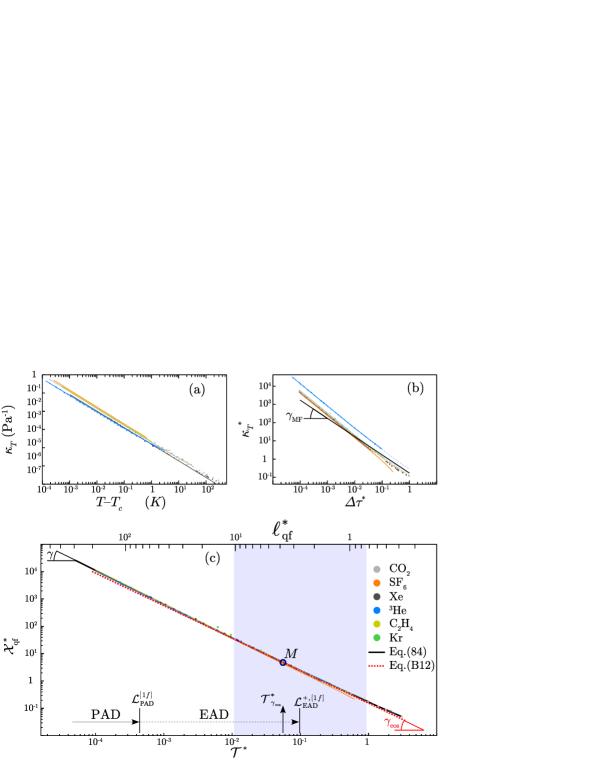
Figure 1: (Color online) Singular behavior of the isothermal compressibility of the one-component fluids. (a) $\kappa_{T}$ as a function of $T-T_{c}>0$ (log-log scale), along the critical isochore for Xe, Kr, ³He, SF₆, CO₂, and C₂H₄ (see inserted Table for fluid color indexation); (b) Log-Log plot of $\kappa_{T}^{*}\left(\Delta\tau^{*}\right)$; black full curve: mean-field behavior of equation $\kappa_{T,\text{vdW}}^{*}=\frac{1}{6}\left(\Delta\tau^{*}\right)^{-\gamma_{\text{MF}}}$ with $\gamma_{\text{MF}}=1$. (c) Matched master behavior (log-log scale) of the renormalized susceptibility $\mathcal{X}_{\text{qf}}^{*}=\left(\Lambda_{qe}^{*}\right)^{2-d}Z_{c}\kappa_{T}^{*}$ [see Eqs. (31)], as a function of the renormalized thermal field $\mathcal{T}^{*}$ [see Eqs. (22)]; black full curve: Eq. (84); red dashed curve: tangent of Eq. (128) at the point M (see text and Appendix B); (full) arrow (label PAD): master extension of the Ising like preasymptotic domain of Eq. (100); (dashed) arrow (label EAD): effective extension of the extended asymptotic domain of Eq. (111) corresponding to $\ell_{\text{qf}}^{\ast}=\left(\Lambda_{qe}^{*}\right)^{-1}\frac{\xi}{\alpha_{c}}\gtrsim 3$ (see Ref. Garrabos2006corlength ); grey area: master correlation length range $10.5\lesssim\ell_{\text{qf}}^{\ast}\lesssim 0.73$ (thermal field range $1.9\times 10^{-2}\lesssim\mathcal{T}^{*}\lesssim 1$) discussed in Appendix B .

A detailed presentation of the scale dilatation method can be found in references Garrabos1982 ; Garrabos1985 ; Garrabos1986 ; Garrabos2002 ; Garrabos2006qe . Hereafter we only recall the main features which close the master description of the singular behaviors of the $\left\{1f\right\}$-subclass within the preasymptotic domain (with $\gamma$, $\nu$, and $\Delta$ selected as independent critical exponents). The scale dilatation method uses explicit analytical transformations of each physical field $\Delta\tau^{*}$ and $\Delta h^{*}$ given by the equations

$$\mathcal{T}_{\text{qf}}^{*}\equiv\mathcal{T}^{*}=Y_{c}\left|\Delta\tau^{*}\right|$$ (22)

$$\mathcal{H}_{\text{qf}}^{*}=\left(\Lambda_{qe}^{*}\right)^{2}\mathcal{H}^{*}=\left(\Lambda_{qe}^{*}\right)^{2}\left(Z_{c}\right)^{-\frac{d}{2}}\left|\Delta h^{*}\right|$$ (23)

where $\mathcal{T}_{\text{qf}}^{*}\equiv\mathcal{T}^{*}$ is the renormalized thermal field, and $\mathcal{H}_{\text{qf}}^{*}$ is the renormalized ordering field. The subscript qf distinguishes between a quantity which refers to a quantum fluid (i.e., $\Lambda_{qe}^{*}\neq 1$) from the one which refers to a non-quantum fluid (i.e., $\Lambda_{qe}^{*}=1$) Garrabos2006qe . Accordingly, the analytic transformation between the physical order parameter density $\Delta m^{*}$ and the renormalized order parameter density $\mathcal{M}_{\mbox{qf}}^{*}$, reads as follows Garrabos1985 ; Garrabos2002 ; Garrabos2006qe

$$\mathcal{M}_{\text{qf}}^{*}=\Lambda_{qe}^{*}\mathcal{M}^{*}=\Lambda_{qe}^{*}\left(Z_{c}\right)^{\frac{d}{2}}\left|\Delta m^{\ast}\right|$$ (24)

Introducing then the dimensionless correlation length $\xi^{\ast}=\frac{\xi}{\alpha_{c}}$, the renormalized correlation length $\ell_{\text{qf}}^{\ast}$ is given by the equation

$$\ell_{\text{qf}}^{\ast}=\left(\Lambda_{qe}^{\ast}\right)^{-1}\ell^{\ast}=\left(\Lambda_{qe}^{\ast}\right)^{-1}\xi^{\ast}$$ (25)

which preserves the same length unit for thermodynamic and correlations functions (with $\ell^{\ast}\equiv\xi^{\ast}$ for the non-quantum fluid case).

The master asymptotic singular behavior of $\ell_{\text{qf}}^{\ast}\left(\mathcal{T}^{\ast}\right)$ was studied in Garrabos2006corlength . Specifically, the observed asymptotic divergence of $\ell_{\text{qf}}^{\ast}$ was represented by the following (two-term) Wegner expansion

$$\ell_{\text{qf}}^{\ast}=\mathcal{Z}_{\xi}^{+}\left(\mathcal{T}^{\ast}\right)^{-\nu}\left[1+\mathcal{Z}_{\xi}^{1,+}\left(\mathcal{T}^{\ast}\right)^{\Delta}\right]$$ (26)

where $\nu=0.6303875$ and $\Delta=0.50189$ Guida1998 . The leading amplitude $\mathcal{Z}_{\xi}^{+}=0.570481$ and the first confluent amplitude $\mathcal{Z}_{\xi}^{1,+}=0.37695$ have master (i.e. unique) values for the $\left\{1f\right\}$-subclass. The associated asymptotic singular behavior of the physical correlation length was given by

$$\xi_{\text{exp}}\left(\Delta\tau^{*}\right)=\xi_{0}^{+}\left(\Delta\tau^{*}\right)^{-\nu}\left[1+a_{\xi}^{+}\left(\Delta\tau^{*}\right)^{\Delta}\right]$$ (27)

Therefore, the term to term comparison of (master) Eq. (26) and (physical) Eq. (27), results in the following amplitude combinations

$$\frac{\xi_{0}^{+}}{\alpha_{c}}=\xi^{+}=\Lambda_{qe}^{*}\left(Y_{c}\right)^{-\nu}\mathcal{Z}_{\mathcal{\xi}}^{+}$$ (28)

$$a_{\xi}^{+}=\mathcal{Z}_{\xi}^{1,+}\left(Y_{c}\right)^{\Delta}$$ (29)

Applying now the scale dilatation method to any physical (thermodynamic) property $P\left(\Delta\tau^{*}\right)$, the master singular behavior for the renormalized (thermodynamic) property $\mathcal{P}_{\text{qf}}^{\ast}\left(\mathcal{T}^{*}\right)$ can be also observed and represented within the preasymptotic domain by the restricted expansion

$$\mathcal{P}_{\text{qf}}^{\ast}=\mathcal{Z}_{P}^{\pm}\left(\mathcal{T}^{*}\right)^{-e_{P}}\left[1+\mathcal{Z}_{P}^{1,\pm}\left(\mathcal{T}^{*}\right)^{\Delta}\right]$$ (30)

where $\mathcal{Z}_{P}^{\pm}$ and $\mathcal{Z}_{P}^{1\pm}$ are two master constants for any one-component fluid (see Table 1). To close the master description in conformity with the universal features estimated within this Ising-like preasymptotic domain, we complete the representation of the master correlation length with the one of the master susceptibility $\mathcal{X}_{\text{qf}}^{*}$ obtained from master order parameter density $\mathcal{M}_{\text{qf}}^{*}$, and master ordering field $\mathcal{H}_{\text{qf}}^{*}$, using the thermodynamic definition, $\mathcal{X}_{\text{qf}}^{*}=\left(\frac{\partial\mathcal{M}_{\text{qf}}^{*}}{\partial\mathcal{H}_{\text{qf}}^{*}}\right)_{\mathcal{T}^{*}}$. $\mathcal{X}_{\text{qf}}^{*}$ is related to the dimensionless isothermal susceptibility $\chi_{T}^{*}=\left(\frac{\partial\left(\Delta m^{*}\right)}{\partial\left(\Delta h^{*}\right)}\right)_{\Delta\tau^{*}}$ by the following equations,

$$\begin{array}[]{rl}\mathcal{X}_{\text{qf}}^{*}&=\left(\Lambda_{qe}^{*}\right)^{2-d}\varkappa_{\mathcal{T}}^{*}\\ &=\left(\Lambda_{qe}^{*}\right)^{2-d}\left(Z_{c}\right)^{d}\chi_{T}^{*}\end{array}$$ (31)

As previously mentioned for the critical isochore case, $\chi_{T}^{*}\left(n_{c}^{*}\right)=\frac{\tilde{\chi}_{T}\left(\tilde{\rho}=1\right)}{\left(Z_{c}\right)^{2}}$, while $\tilde{\chi}_{T}\left(\tilde{\rho}=1\right)\equiv\kappa_{T}^{*}(\tilde{\rho}=1)$ [with $\tilde{\chi}_{T}=\left(\frac{\partial\left(\Delta\tilde{\rho}\right)}{\partial\left(\Delta\tilde{\mu}\right)}\right)_{\Delta\tau^{*}}=\left(\tilde{\rho}\right)^{2}\kappa_{T}^{*}$], where $\kappa_{T}^{*}$ is the dimensionless isothermal compressibility $\kappa_{T}^{*}=\frac{1}{\beta_{c}\left(\alpha_{c}\right)^{d}}\left[\frac{1}{\rho}\left(\frac{\partial\rho}{\partial p}\right)_{T}\right]=p_{c}\kappa_{T}$ (with $\kappa_{T}=\frac{1}{\rho}\left(\frac{\partial\rho}{\partial p}\right)_{T}$). Therefore, the master susceptibility can be also related to the dimensionless isothermal compressibility by,

$$\mathcal{X}_{\text{qf}}^{*}=\left(\Lambda_{qe}^{*}\right)^{2-d}Z_{c}\kappa_{T}^{*}$$ (32)

The master asymptotic singular behavior of $\mathcal{X}_{\text{qf}}^{*}$ reads as follows

$$\mathcal{X}_{\text{qf}}^{*}=\mathcal{Z}_{\chi}^{+}\left(\mathcal{T}^{*}\right)^{-\gamma}\left[1+\mathcal{Z}_{\chi}^{1,+}\left(\mathcal{T}^{*}\right)^{\Delta}\right]$$ (33)

where $\gamma=1.2396935$ Guida1998 . The master values of the leading and confluent amplitudes are $\mathcal{Z}_{\chi}^{+}=0.119$ and $\mathcal{Z}_{\chi}^{1,+}=0.555$, respectively, where the universal value of the confluent amplitude ratio $\frac{\mathbb{\mathcal{Z}}_{\xi}^{1,+}}{\mathbb{\mathcal{Z}}_{\chi}^{1,+}}=0.67919$ is given in Ref. Bagnuls2002 . The associated asymptotic singular behavior of the isothermal compressibility reads as follows

$$\kappa_{T,\text{exp}}^{*}\left(\Delta\tau^{*}\right)=\Gamma^{+}\left(\Delta\tau^{*}\right)^{-\gamma}\left[1+a_{\chi}^{+}\left(\Delta\tau^{*}\right)^{\Delta}\right]$$ (34)

The term to term comparison of (master) Eq. (33) and (physical) Eq. (34), leads to the following amplitude estimations

$$\Gamma^{+}=\left(\Lambda_{qe}^{*}\right)^{d-2}\left(Z_{c}\right)^{-1}\left(Y_{c}\right)^{-\gamma}\mathcal{Z}_{\chi}^{+}$$ (35)

$$a_{\chi}^{+}=\mathcal{Z}_{\chi}^{1+}\left(Y_{c}\right)^{\Delta}$$ (36)

with

$$\frac{\mathbb{\mathcal{Z}}_{\xi}^{1,+}}{\mathbb{\mathcal{Z}}_{\chi}^{1,+}}=\frac{a_{\xi}^{+}}{a_{\chi}^{+}}=0.67919$$ (37)

The expected asymptotic collapse of the fluid properties on a single curve due to the scale dilatation method is illustrated in Fig. 1 (log-log scale). The raw data are reported in Fig. 1a to easily distinguish between singular behavior of $\kappa_{T}$ (expressed in $\text{Pa}^{-1}$) as a function of $T-T_{c}$ (expressed in K), for each one-component fluid (see the fluid color indexation inserted in Fig. 1c). Figure 1b illustrates the differences between the corresponding dimensionless behaviors $\kappa_{T}^{*}\left(\Delta\tau^{*}\right)$ which confirm the failure of results provided by the two-parameter corresponding state principle. This figure also shows the failure of mean-field like behavior predicted from the van der Waals (vdW) equation of state which is here represented by the black full curve of equation $\kappa_{T,\text{vdW}}^{*}\left(\Delta\tau^{*}\right)^{\gamma_{\text{vdW}}}=\Gamma_{\text{vdW}}^{+}=\frac{1}{6}$, with $\gamma_{\text{vdW}}=\gamma_{\text{MF}}=1$. On the other hand, Fig. 1c demonstrates the collapse of $\mathcal{X}_{\text{qf}}^{*}\left(\mathcal{T}^{*}\right)$ on a master curve where the scatter corresponds to the estimated $\kappa_{T}$-precision (5-10%) for each fluid. We underline the combination of the “scaling” and “extensive” roles of the characteristic factor $Z_{c}$ in the renormalization [see Eqs. (31) and (32)] of the ordinate axis of Fig. 1c (compare for example with Fig. 3 of Ref. Luijten2000 or with Fig. 2 of Ref. Hahn2001 ). The complementary materials for complete analysis of this Fig. 1c will be given below and in Appendix B.

Therefore, adding the correlation length results given in Fig. 1c of Ref. Garrabos2006corlength to the present isothermal susceptibility results, we close the asymptotic master behavior generated by the scale dilatation method, in conformity with the two-scale-factor universality of the Ising-like systems.

To summarize the main interest of this Ising-like master description of the $\left\{1f\right\}$-subclass (associated to the selected set $\left\{\Delta;\nu;\gamma\right\}$ of three independent universal exponents Guida1998 ), we introduce

i) the physical amplitude set

$$S_{A}=\left\{a_{\chi}^{+};\xi^{+};\Gamma^{+}\right\}$$ (38)

which characterizes the physical Ising-like universal features of each selected pure fluid having the critical set $\left\{Q_{c}^{\text{min}};\Lambda_{qe}^{*}\right\}$;

ii) the corresponding scale factor set

$$S_{SF}=\left\{Y_{c};Z_{c};\Lambda_{qe}^{*}\right\}$$ (39)

which characterizes the dimensional universal features of the critical interaction cell of each selected pure fluid having $\left(\beta_{c}\right)^{-1}$ and $\alpha_{c}$ as energy and length units, respectively, and

iii) the master amplitude set,

$$\mathcal{S}_{A}^{\left\{1f\right\}}=\left\{\begin{array}[]{cl}\mathcal{Z}_{\chi}^{1,+}=&0.555\\ \mathcal{Z}_{\mathcal{\xi}}^{+}=&0.570481\\ \mathcal{Z}_{\chi}^{+}=&0.119\end{array}\right\}$$ (40)

which characterizes the master Ising-like universal features of the $\left\{1f\right\}$-subclass. Three independent relations, i.e., [Eqs. (28), (35), and (36)], connecting these three previous sets, can be written in the following condensed functional form

$$\mathcal{S}_{A}^{\left\{1f\right\}}=\left\{S_{A}\,\mathcal{F}\left(S_{SF}\right)\right\}_{\left(\beta_{c}\right)^{-1},\alpha_{c},\Lambda_{qe}^{*}}$$ (41)

where the function $\mathcal{F}\left(S_{SF}\right)$ takes an universal scaling form of the two (fluid-dependent) scale factors $Y_{c}$ and $Z_{c}$. Accordingly, any physical amplitude of any one-component fluid can be estimated from the equations given in Table 1 satisfying to the two-scale-factor universality of the $\left\{\Phi_{3}\left(1\right)\right\}$-class (where xenon acts as a standard critical fluid to estimate three characteristic master amplitudes labeled with an asterisk, see Refs. Garrabos1985 ; Garrabos1986 ; Garrabos2006khiT ). However, the effective extension range where the master behavior is observed, as an explicit criteria which defines the preasymptotic range where the two-term Wegner-like expansion is valid, remain not easy to estimate precisely only using the scale dilatation method. These two problems can be solved using a master modification of the mean crossover functions Garrabos2006gb obtained from the massive renormalization scheme, as shown in the next section.

III Master modifications of the mean crossover functions

III.1 System-dependent parameters of the mean crossover functions.

For the $\left\{\Phi_{3}\left(1\right)\right\}$-class, the mean crossover functions $F_{P}\left(t,h=0\right)$ describing the crossover behavior of the theoretical properties $P_{\text{th}}\left(t\right)$ as a function of the renormalized temperature-like field $t$, for zero value of the external ordering (magnetic-like) field $h$, are given in detail in I. All the theoretical functions $F_{P}\left(t\right)$ have the same functional form whatever $P_{\text{th}}$, and, as noted in I, a closed presentation of their universal features, only needs to use for example the mean crossover functions $F_{\ell}\left(t\right)=\frac{1}{\ell_{\text{th}}\left(t\right)}$ for the inverse correlation length, and $F_{\chi}\left(t\right)=\frac{1}{\chi_{\text{th}}\left(t\right)}$ for the inverse susceptibility, at $h=0$, in the homogeneous phase $T>T_{c}$ [$T$ ($T_{c}$) is the temperature (critical temperature)]. These two theoretical functions read as follows:

$$\left[\ell_{\text{th}}\left(t\right)\right]^{-1}=\mathbb{Z}_{\xi}^{+}t^{\nu}{\displaystyle\prod_{i=1}^{3}\left(1+X_{\xi,i}^{+}t^{D\left(t\right)}\right)^{Y_{\xi,i}^{+}}}$$ (42)

$$\left[\mathcal{X}_{\text{th}}\left(t\right)\right]^{-1}=\mathbb{Z}_{\chi}^{+}t^{\gamma}{\displaystyle\prod_{i=1}^{3}\left(1+X_{\chi,i}^{+}t^{D\left(t\right)}\right)^{Y_{\chi,i}^{+}}}$$ (43)

$D\left(t\right)$ is a universal mean crossover function for the confluent exponents $\Delta$ and $\Delta_{\text{MF}}$ which reads

$$D\left(t^{*}\right)=\frac{\Delta_{\text{MF}}S_{2}\sqrt{t}+\Delta}{S_{2}\sqrt{t}+1}$$ (44)

such that $D\left(t=\frac{1}{\left(S_{2}\right)^{2}}\right)=\frac{\Delta_{\text{MF}}+\Delta}{2}$. All the universal exponents $\nu$, $\gamma$, $\Delta$, $\Delta_{\text{MF}}$, and the parameters $\mathbb{Z}_{\xi}^{+}$, $X_{\xi,i}^{+}$, $Y_{\xi,i}^{+}$, $\mathbb{Z}_{\chi}^{+}$, $X_{\chi,i}^{+}$, $Y_{\chi,i}^{+}$, and $S_{2}$, are given in I.

The temperature-like field $t$ is analytically related to the physical dimensionless temperature distance

$$\Delta\tau^{*}=\frac{T-T_{c}}{T_{c}}$$ (45)

by the following linear approximation

$$t=\vartheta\Delta\tau^{*}$$ (46)

which introduces $\vartheta$ as an adjustable (system-dependent) parameter. Here $\vartheta$ is a scale factor for the temperature field. Correlatively, it is important to note that the definition of $\Delta\tau^{*}$ [see Eq. (45)], introduces the critical temperature $T_{c}$ as a system-dependent parameter. Then the relation between the dimensionless thermodynamic free energies of the $\Phi^{4}$-model and the physical (one-component fluid) system, only involves the energy unit $\left(\beta_{c}\right)^{-1}=k_{B}T_{c}$.

Similarly, the ordering-like field $h$ is analytically related to the corresponding physical dimensionless variables $\Delta\tilde{\mu}$ (or $\Delta h^{*}$) by the following linear approximations (including quantum effects)

$$\begin{array}[]{rl}h&=\psi_{\rho}\left[\left(\Lambda_{qe}^{*}\right)^{2}\Delta\tilde{\mu}\right]\\ \text{or}\>h&=\psi\left[\left(\Lambda_{qe}^{*}\right)^{2}\Delta h^{*}\right]\end{array}$$ (47)

which introduce $\psi_{\rho}$ (or $\psi$) as an adjustable (system-dependent) parameter. $\psi_{\rho}$, respectively $\psi=\left(Z_{c}\right)^{-1}\psi_{\rho}$, is a scale factor for the ordering field $\Delta\tilde{\mu}$, respectively $\Delta h^{*}=Z_{c}\Delta\tilde{\mu}$.

Accordingly, the dimensional analysis of each term of the dimensionless hamiltonian of the $\Phi^{4}$-model leads to the introduction of a finite arbitrary wave-vector $\Lambda_{0}$, so-called the cutoff parameter, which is related to the finite short range of the microscopic interaction (see for example, Ref. Bagnuls1984a ). Since the value of the cutoff parameter of a selected physical system is generally unknown, a convenient method at $d=3$ consists in replacing $\Lambda_{0}$ by $g_{0}$ Bagnuls1984b ; Garrabos2006gb , which is the critical coupling constant having the correct wavenumber dimension (see our introductive part). This system-dependent wavenumber $g_{0}$ provides the practical “adjustable” link between the theoretical dimensionless correlation length ($\ell_{\text{th}}$) and the measured physical correlation length ($\xi_{\text{exp}}$) of the system at $d=3$, through the fitting equation :

$$\left(\Lambda_{qe}^{*}\right)^{-1}\xi_{\text{exp}}\left(\Delta\tau^{*}\right)=\left(g_{0}\right)^{-1}\ell_{\text{th}}\left(t\right)$$ (48)

In Eq. (48), $\left(g_{0}\right)^{-1}$ appears as a metric prefactor for the theoretical correlation length function. From Eqs. (46), (47), and (48), the asymptotical non-universal nature of each physical system is then characterized by the scale factor set $\left\{\vartheta;\left(g_{0}\right)^{-1};\psi_{\rho}\,\left(or\,\psi\right)\right\}$ (with implicit knowledge of $T_{c}$ and $\Lambda_{qe}^{*}$). However, for the present fluid study where the thermodynamic length unit is already fixed by Eq. (5), the above fitting Eq. (48) introduces one supplementary dimensionless number defined such as:

$$\mathbb{L}^{\left\{1f\right\}}=g_{0}\alpha_{c}$$ (49)

where the notation $\mathbb{L}^{\left\{1f\right\}}$ anticipates a master nature of this product which we will demonstrate below [see Eq. (93)]. More generally, in order to maintain unicity of the length unit in the dimensionless description of the singular behavior, any theroretical density property (which implicitely refers to the length scale unit $\left(g_{0}\right)^{-1}$) needs to introduce the proportionality factor $\left(\mathbb{L}^{\left\{1f\right\}}\right)^{-d}$ to the corresponding dimensionless physical density which refers to the length scale unit $\alpha_{c}$. As a direct consequence of the fitting Eq. (48) for the correlation length, the order parameter density $m$ must be analytically related to the corresponding physical dimensionless variables $\Delta\tilde{\rho}$ (or $\Delta m^{*}$) by the following linear approximation (including quantum effects)

$$\begin{array}[]{rl}m&=\left(\mathbb{L}^{\left\{1f\right\}}\right)^{-d}\left(\psi_{\rho}\right)^{-1}\left[\Lambda_{qe}^{*}\Delta\tilde{\rho}\right]\\ or\,m&=\left(\mathbb{L}^{\left\{1f\right\}}\right)^{-d}\psi^{-1}\left[\Lambda_{qe}^{*}\Delta m^{*}\right]\end{array}$$ (50)

For simplification of the following presentation, we only use $\psi_{\rho}$ related to the practical dimensionless form of the variables (see above § 2.3).

Finally, adding the knowledge of the energy unit and the length unit for each pure fluid to the theoretical results obtained from the massive renormalization scheme, the dimensionless singular behaviors of the fluid properties are now characterized by the set

$$\mathbb{S}_{SF}=\left\{\vartheta;\mathbb{L}^{\left\{1f\right\}};\psi_{\rho}\right\}$$ (51)

made of three dimensionless scale factors (admitting that $\left(\beta_{c}\right)^{-1}$, $\alpha_{c}$, and $\Lambda_{qe}^{*}$ are known). Therefore, it is easy to analytically define these three dimensionless parameters which characterize each Ising-like fluid, thanks to the exact values of the mean crossover functions within this preasymptotic domain.

III.2 Three scale-factor characterization within the Ising-like preasymptotic domain.

As already mentionned in the introduction and discussed in a detailed manner in I, this asymptotic characterization is valid within the Ising-like preasymptotic domain where the complete crossover functions of Eqs. (42) and (43) can be approximated by the following restricted (two-term) Wegner-like expansions Wegner1972 :

$$\ell_{\text{PAD,th}}\left(t\right)=\left(\mathbb{Z}_{\xi}^{+}\right)^{-1}t^{-\nu}{\displaystyle\left[1+\mathbb{Z}_{\xi}^{1,+}t^{\Delta}\right]}$$ (52)

$$\mathcal{X}_{\text{\text{PAD},th}}\left(t\right)=\left(\mathbb{Z}_{\chi}^{+}\right)^{-1}t^{-\gamma}{\displaystyle\left[1+\mathbb{Z}_{\chi}^{1,+}t^{\Delta}\right]}$$ (53)

In Eqs. (52) and (53), $\mathbb{Z}_{\xi}^{1,+}$ [see below Eq. (54)], is the amplitude of the first confluent correction to scaling for the correlation length, which is related to the one for the susceptibility $\mathbb{Z}_{\chi}^{1,+}$ [see below Eq. (55)], by the universal ratio $\frac{\mathbb{Z}_{\xi}^{1,+}}{\mathbb{Z}_{\chi}^{1,+}}=0.67919$ Bagnuls2002 , with:

$$\mathbb{Z}_{\xi}^{1,+}=-{\displaystyle\sum_{i=1}^{3}}X_{\xi,i}^{+}Y_{\xi,i}^{+}$$ (54)

$$\mathbb{Z}_{\mathcal{\chi}}^{1,+}=-{\displaystyle\sum_{i=1}^{3}}X_{\chi,i}^{+}Y_{\chi,i}^{+}$$ (55)

The theoretical field extension $t\lesssim\mathcal{L}_{\text{PAD}}^{\text{Ising}}$ of the Ising-like preasymptotic domain where the restricted Eqs. (52) and (53) are valid is defined in I, such as

$$\mathcal{L}_{\text{PAD}}^{\text{Ising}}=\frac{10^{-3}}{\left(S_{2}\right)^{2}}\approx 1.9\,10^{-6}$$ (56)

Now considering all the theoretical functions estimated for all the singular properties of the Ising-like systems (see I), we can note that the universal features in the Ising-like preasymptotic domain are characterized by the set

$$\mathcal{\mathbb{S}}_{A}^{\left\{MR\right\}}=\left\{\begin{array}[]{rl}\mathbb{Z}_{\chi}^{1,+}=&8.56347\\ \left(\mathbb{Z}_{\xi}^{+}\right)^{-1}=&0.471474\\ \left(\mathbb{Z}_{\chi}^{+}\right)^{-1}=&0.269571\end{array}\right\}$$ (57)

of three theoretical amplitudes associated to the set $\left\{\Delta;\nu;\gamma\right\}$ of three universal exponents selected as independent. Accordingly, the restricted forms of two independent fitting equations are

$$\begin{array}[]{cc}\left(\Lambda_{qe}^{*}\right)^{-1}\frac{\xi_{\text{exp}}}{\alpha_{c}}=&\left(\mathbb{L}^{\left\{1f\right\}}\right)^{-1}\left(\mathbb{Z}_{\xi}^{+}\right)^{-1}\left(\vartheta\Delta\tau^{*}\right)^{-\nu}\\ &{\displaystyle\left[1+\mathbb{Z}_{\xi}^{1,+}\left(\vartheta\Delta\tau^{*}\right)^{\Delta}\right]}\end{array}$$ (58)

$$\begin{array}[]{cc}\left(\Lambda_{qe}^{*}\right)^{2}\kappa_{T,\text{exp}}^{*}=&\left(\mathbb{L}^{\left\{1f\right\}}\right)^{d}\left(\psi_{\rho}\right)^{2}\left(\mathbb{Z}_{\chi}^{+}\right)^{-1}\left(\vartheta\Delta\tau^{*}\right)^{-\gamma}\\ &\left[1+\mathbb{Z}_{\mathcal{\chi}}^{1,+}\left(\vartheta\Delta\tau^{*}\right)^{\Delta}\right]\end{array}$$ (59)

where $\xi_{\text{exp}}$ and $\kappa_{T,\text{exp}}^{*}$ are given by the restricted Wegner-like expansions of Eqs. (27) and (34), respectively. That provides the following hierarchical relations

$$a_{\chi}^{+}=\mathbb{Z}_{\mathcal{\chi}}^{1,+}\vartheta^{\Delta}$$ (60)

$$\frac{\xi_{0}^{+}}{\alpha_{c}}=\xi^{+}=\left(\mathbb{Z}_{\xi}^{+}\right)^{-1}\left(\mathbb{L}^{\left\{1f\right\}}\right)^{-1}\Lambda_{qe}^{*}\vartheta^{-\nu}$$ (61)

$$\Gamma^{+}=\left(\mathbb{Z}_{\chi}^{+}\right)^{-1}\left(\mathbb{L}^{\left\{1f\right\}}\right)^{d}\left(\Lambda_{qe}^{*}\right)^{d-2}\left(\psi_{\rho}\right)^{2}\vartheta^{-\gamma}$$ (62)

with $\frac{a_{\xi}^{+}}{a_{\chi}^{+}}=\frac{\mathbb{Z}_{\xi}^{1,+}}{\mathbb{Z}_{\mathcal{\chi}}^{1,+}}=0.67919$ Guida1998 ; Bagnuls2002 . We underline the fact that Eq. (60) (or equivalently equation $a_{\xi}^{+}=\mathbb{Z}_{\mathcal{\xi}}^{1,+}\vartheta^{\Delta}$ in the correlation length case), is to be first validated (to confer unequivocal Ising-like equivalence between the first (system-dependent) scale factor $\vartheta$ and $a_{\chi}^{+}$). Then Eq. (61) fixes the asymptotic amplitude of the dimensionless correlation length and generates a single scale factor attached to the selected (physical) length unit, which is then mandatory common to the thermodynamic and correlations functions. Finally, the validation of Eq. (62) provides unequivocal Ising-like equivalence between the second (system-dependent) scale factor $\psi_{\rho}$ and $\Gamma^{+}$ (accounting for “critical” and “extensive” nature of the susceptibility).

Equations (60) to (62) satisfy the following condensed functional form

$$\mathcal{\mathbb{S}}_{A}^{\left\{MR\right\}}=\left\{S_{A}\,\mathbb{F}\left(\mathbb{S}_{SF}\right)\right\}_{\left(\beta_{c}\right)^{-1},\alpha_{c},\Lambda_{qe}^{*}}$$ (63)

where the function $\mathbb{F}$ takes an universal scaling form of the dimensionless asymptotic scale factors $\vartheta$ and $\psi_{\rho}$. The universal character of Eq. (63) occurs for any one-parameter crossover modeling. That infers Ising-like equivalence between all estimated crossover functions only using three model-dependent characteristic numbers. This result is shown in Appendix A, considering the asymptotic crossover infered by the minimal-subtraction renormalization scheme MSRscheme ; Zhong2003 and the phenomenological approach given by a parametric model of the equation of state Agayan2001 .

Obviously, from Eqs. (46) and (56), it is easy to define the extension range

$$\Delta\tau^{*}<\mathcal{L}_{\text{PAD}}^{f}=\frac{\mathcal{L}_{\text{PAD}}^{\text{Ising}}}{\vartheta}\simeq\frac{1.9\times 10^{-6}}{\vartheta}$$ (64)

of the Ising-like preasymptotic domain of the selected fluid (labeled with superscript $f$). Therefore, for each one-component fluid for which $\vartheta$ (or equivalently one confluent amplitude among $a_{\chi}^{+}$ or $a_{\xi}^{+}$) is an unknown parameter, the remaining question of concern is: How to define the validity range $\Delta\tau^{*}<\mathcal{L}_{\text{PAD}}^{f}$ where the theoretical Ising-like characterization by three scale factors can replace the experimental characterization by three asymptotic amplitudes?

III.3 Three free-parameter characterization beyond the Ising-like preasymptotic domain

As noted in Ref. Bagnuls2002 , in the absence of information concerning the true extension of the Ising-like behavior for a real system belonging to the 3D Ising-like universality class, the introduction of the scale factors $\vartheta$, $\psi_{\rho}$, and the wavelength unit $g_{0}$ throughout Eqs. (46) to (48) cannot be easily controlled. Alternatively, it was proposed to introduce three adjustable dimensionless parameters $\mathbb{L}_{0,\mathcal{L}}^{*}$, $\mathbb{X}_{0,\mathcal{L}}^{*}$, and $\vartheta_{\mathcal{L}}$, using the following fitting equations:

$$\begin{array}[]{cl}\frac{\alpha_{c}}{\xi_{\text{exp}}^{*}\left(\Delta\tau^{*}\right)}=&\left(\mathbb{L}_{0,\mathcal{L}}^{*}\right)^{-1}\mathbb{Z}_{\xi}^{+}\left(\Delta\tau^{*}\right)^{\nu}\\ &\prod_{i=1}^{K}\left(1+X_{\xi,i}^{+}\left(t\right)^{D\left(t\right)}\right)^{Y_{\xi,i}^{+}}\end{array}$$ (65)

$$\begin{array}[]{cl}\frac{1}{\kappa_{T,\text{exp}}^{*}\left(\Delta\tau^{*}\right)}=&\left(\mathbb{X}_{0,\mathcal{L}}^{*}\right)^{-1}\mathbb{Z}_{\mathcal{\chi}}^{+}\left(\Delta\tau^{*}\right)^{\gamma}\\ &\prod_{i=1}^{K}\left(1+X_{\mathcal{\chi},i}^{+}\left(t\right)^{D\left(t\right)}\right)^{Y_{X,i}^{+}}\end{array}$$ (66)

with

$$t=\vartheta_{\mathcal{L}}\Delta\tau^{*}$$ (67)

$\mathbb{L}_{0,\mathcal{L}}^{*}$ and $\mathbb{X}_{0,\mathcal{L}}^{*}$ are two adjustable metric prefactors (with same value above and below $T_{c}$). $\vartheta_{\mathcal{L}}$ is a global crossover parameter in a sense where it is attached to an unknown effective parameter $\mathcal{L}^{f}$ which measures the extent of fitting agreement involving an undefined number of terms in the Wegner-like expansion (see I for details). The determination of $\vartheta_{\mathcal{L}}$ is then equivalent to the determination of $\mathcal{L}^{f}$. However, within the Ising-like preasymptotic domain, the restricted forms of the fitting Eqs. (65) and (66) are

$$\frac{\xi_{\text{exp}}}{\alpha_{c}}=\mathbb{L}_{0,\mathcal{L}}^{*}\left(\mathbb{Z}_{\xi}^{+}\right)^{-1}\left(\Delta\tau^{*}\right)^{-\nu}{\displaystyle\left[1+\mathbb{Z}_{\xi}^{1,+}\left(\vartheta_{\mathcal{L}}\Delta\tau^{*}\right)^{\Delta}\right]}$$ (68)

$$\kappa_{T,\text{exp}}^{*}=\mathbb{X}_{0,\mathcal{L}}^{*}\left(\mathbb{Z}_{\chi}^{+}\right)^{-1}\left(\Delta\tau^{*}\right)^{-\gamma}{\displaystyle\left[1+\mathbb{Z}_{\mathcal{\chi}}^{1,+}\left(\vartheta_{\mathcal{L}}\Delta\tau^{*}\right)^{\Delta}\right]}$$ (69)

Therefore, the physical leading amplitudes can be calculated using the (independent) equations:

$$\frac{\xi_{0}^{+}}{\alpha_{c}}=\mathbb{L}_{0,\mathcal{L}}^{*}\left(\mathbb{Z}_{\xi}^{+}\right)^{-1}$$ (70)

$$\Gamma^{+}=\mathbb{X}_{0,\mathcal{L}}^{*}\left(\mathbb{Z}_{\chi}^{+}\right)^{-1}$$ (71)

i.e., without explicit reference to $\vartheta_{\mathcal{L}}$ (however the subscript $\mathcal{L}$ recalls for the implicit $\vartheta_{\mathcal{L}}$ dependence due to the fitting in the temperature range $\Delta\tau^{*}\leq\mathcal{L}^{f}$, with $\mathcal{L}^{f}>\mathcal{L}_{\text{PAD}}^{f}$). Noticeable distinction occurs for the confluent corrections to scaling since the first confluent amplitudes are only $\vartheta_{\mathcal{L}}$-dependent and can be calculated using the equations:

$$a_{\xi}^{+}=\left(\vartheta_{\mathcal{L}}\right)^{\Delta}\mathbb{Z}_{\xi}^{1,+}$$ (72)

$$a_{\chi}^{+}=\left(\vartheta_{\mathcal{L}}\right)^{\Delta}\mathbb{Z}_{\mathcal{\chi}}^{1,+}$$ (73)

interrelated by the universal ratio $\frac{\mathbb{Z}_{\xi}^{1,+}}{\mathbb{Z}_{\chi}^{1,+}}=0.67919$ Bagnuls2002 .

For better understanding of the scaling nature of the analytical transformations of the physical variables [such as Eqs. (46) or (67)], we select Eq. (73) as the independent equation for the critical crossover characterization. We must then rewrite the above Eqs. (70) to (73) in the following hierarchical forms

$$\left(\vartheta_{\mathcal{L}}\right)^{-\Delta}a_{\chi}^{+}=\mathbb{Z}_{\mathcal{\chi}}^{1,+}=\text{universal}\,\text{cst.}$$ (74)

$$\left(\mathbb{L}_{0,\mathcal{L}}^{*}\right)^{-1}\frac{\xi_{0}^{+}}{\alpha_{c}}=\left(\mathbb{Z}_{\xi}^{+}\right)^{-1}=\text{universal}\,\text{cst.}$$ (75)

$$\left(\mathbb{X}_{0,\mathcal{L}}^{*}\right)^{-1}\Gamma^{+}=\left(\mathbb{Z}_{\mathcal{\chi}}^{+}\right)^{-1}=\text{universal}\,\text{cst.}$$ (76)

where the l.h.s. of the above equations contain all the system-dependent information, first for Ising-like critical crossover, then for asymptotic behavior of correlation functions, and finally for asymptotic behavior of thermodynamic functions. Moreover, this information is given in a dual form, i.e., as a product between a “physical” amplitude ($a_{\chi}^{+}$, $\xi^{+}$, or $\Gamma^{+}$) and either a “crossover” factor ($\vartheta_{\mathcal{L}}$), which acts as a scale factor for the confluent correction contribution, or a “pre”-factor ($\mathbb{L}_{0,\mathcal{L}}^{*}$ or $\mathbb{X}_{0,\mathcal{L}}^{*}$) which acts as a simple factor of proportionality for the corresponding leading amplitude ($\xi^{+}$ or $\Gamma^{+}$). The following set

$$\mathbb{S}_{1C,\mathcal{L}}=\left\{\vartheta_{\mathcal{L}};\mathbb{L}_{0,\mathcal{L}}^{*};\mathbb{X}_{0,\mathcal{L}}^{*}\right\}$$ (77)

is equivalent to the previous set $\mathbb{S}_{SF}$ of Eq. (51), except that the subscript $1C,\mathcal{L}$ recalls for a single crossover parameter obtained over an extended temperature range $\mathcal{L}^{f}>\mathcal{L}_{\text{PAD}}^{f}$, beyond the Ising-like preasymptotic domain. The following condensed functional form

$$\mathcal{\mathbb{S}}_{A}^{\left\{MR\right\}}=\left\{S_{A}\,\mathbb{F}_{\mathcal{L}}\left(\mathbb{S}_{1C,\mathcal{L}}\right)\right\}_{\left(\beta_{c}\right)^{-1},\alpha_{c},\Lambda_{qe}^{*}}$$ (78)

can be used in a equivalent scaling manner to Eq. (63) when the crossover parameter $\vartheta_{\mathcal{L}}$ is unique within the $\mathcal{L}^{f}$ range.

To our knowledge, the unicity of the crossover parameter along the critical isochore of a one-component fluid has never been directly evidenced from the singular behavior of the correlation length or any other thermodynamic property. However, from simultaneous fitting analysis of several singular properties of xenon and helium 3, an indirect probe of a single value for one adjustable parameter related to the scale factor $\vartheta$ was obtained, using the crossover functions estimated in the massive renormalization scheme Bagnuls1984b ; Garrabos2006qe and the minimal-subtraction renormalization scheme Zhong2003 ; Zhong2004 . But these results were never used to accurately analyze the expected equivalence between Eqs. (63) and (78), and then to estimate the other two scale factors $\mathbb{L}^{\left\{1f\right\}}$ and $\psi_{\rho}$, which is the only correct way to verify the asymptotic condition $\vartheta=\vartheta_{\mathcal{L}}$ within the Ising-like preasymptotic domain thetaunicity .

An analytic determination of $\vartheta_{\mathcal{L}}$, made beyond the Ising-like preasymptotic domain without use of any adjustable parameter, is under investigation for the case of the isothermal compressibility of xenon Garrabos2006khiT . The main objective is to carefully correlate the local value of this crossover parameter with the local value of the correlation length before to validate its uniqueness by identification with the asymptotic scale factor $\vartheta$, calculated by using Eq. (46). However, such a challenging demonstration of $\vartheta\equiv\vartheta_{\mathcal{L}}$ in the temperature range $\Delta\tau^{*}\leq\mathcal{L}_{\text{EAD}}^{f}$, i.e., within the so-called Ising-like extended asymptotic domain (EAD) in the following, as a formulation of the three-parameter characterization of xenon selected as a standard one-component fluid, remain two preliminary attempts to test the equivalence between Eqs. (63) and (78). That needs to be examinated using a more general approach, as the one proposed below, where we will introduce three master constants which relate unequivocally dimensionless lengths and relevant fields of both (theoretical and master) descriptions, to identify the theoretical crossover of the $\left\{\Phi_{3}\left(1\right)\right\}$-class with the master crossover of the $\left\{1f\right\}$-subclass.

III.4 Identification of the theoretical and master asymptotic scaling within the Ising-like preasymptotic domain

Now, while reconsidering our previous analysis of the relations between physical and master properties, we must rewrite Eqs. (28), (35), and (36), in the following hierarchical forms

$$Y_{c}\left(a_{\chi}^{+}\right)^{-\frac{1}{\Delta}}=\left(\mathcal{Z}_{\chi}^{1,+}\right)^{\frac{1}{\Delta}}=\text{master}\,\text{cst.}$$ (79)

$$\frac{1}{\alpha_{c}}\left(Y_{c}\right)^{\nu}\left[\left(\Lambda_{qe}^{*}\right)^{-1}\xi_{0}^{+}\right]=\mathcal{Z}_{\mathcal{\xi}}^{+}=\text{master}\,\text{cst.}$$ (80)

$$Z_{c}\left(Y_{c}\right)^{\gamma}\left[\left(\Lambda_{qe}^{*}\right)^{2-d}\Gamma^{+}\right]=\mathcal{Z}_{\chi}^{+}=\text{master}\,\text{cst.}$$ (81)

Comparison of Eqs. (74) to (76) with Eqs. (79) to (81), shows that their r.h.s. differences only concern the respective numerical values of the characteristic master set $\mathcal{S}_{A}^{\left\{1f\right\}}$ of Eq. (40), and universal set $\mathcal{\mathbb{S}}_{A}^{\left\{MR\right\}}$ of Eq. (57). For their l.h.s. comparison, neglecting the quantum corrections in a first approach (i.e. fixing $\Lambda_{qe}^{*}=1$), the term to term identification between measurable amplitudes underlines the analogy between the explicit parameter set $\left\{Y_{c};Z_{c}\right\}$, related to the master description, and the implicit one $\left\{\vartheta;\psi_{\rho}\right\}$, related to the massive renormalization description. We can then note that the $\left\{1f\right\}$-master formulation compares to the $\Phi_{3}\left(1\right)$-universal formulation, only if we have correctly accounted for the asymptotic scaling nature of each dimensionless number needed by the massive renormalization scheme. In order to reveal such a scaling nature, it is essential to note that the scale dilatation method replaces the renormalized fields (such as $t$, $h$, $m$, etc.) needed to observe the “universal” behavior of the $\Phi_{3}^{4}\left(1\right)$-universality class, by the $\left\{1f\right\}$-fields (such as, $\mathcal{T}^{*}$, $\mathcal{H}_{\text{qf}}^{*}$, $\mathcal{M}_{\text{qf}}^{*}$, etc.) needed to observe the “master” behavior of $\left\{1f\right\}$-subclass. The common physical variables are $\Delta\tau^{*}$, $\Delta\tilde{\mu}$, and $\Delta\tilde{\rho}$. Therefore, it remains to give explicit forms for the following exchanges between the theoretical variables and the $\left\{1f\right\}$-subclass variables

$$t\rightarrow\mathcal{T}^{*}$$ (82)

$$h\rightarrow\mathcal{H}_{\text{qf}}^{*} or m\rightarrow\mathcal{M}_{\text{qf}}^{*}$$ (83)

(see Ref. Garrabos2006corlength for the correlation length case). The next subsection is dedicated to the isothermal susceptibility case (which then closes the description of the $\left\{1f\right\}$-subclass along the critical isochore in conformity with the universal features estimated for the Ising-like universality class).

(a)	$F_{P}$	$\mathbb{Z}_{P}^{\pm}$	$\mathbb{Z}_{P}^{1,\pm}$
$\mathcal{\mathbb{S}}_{A}^{\left\{MR\right\}}$	(57)	$\left\{\left(\mathbb{Z}_{\xi}^{+}\right)^{-1}=0.471474;\,\left(\mathbb{Z}_{\chi}^{+}\right)^{-1}=0.269571\right\}$	$\mathbb{Z}_{\chi}^{1,+}=8.56347$
(b)	$\mathcal{P}_{\text{qf}}^{\ast}$	$\mathbb{Z}_{P}^{\left\{1f\right\}}$	$\mathbb{\mathcal{Z}}_{P}^{1,\pm}$
$\mathcal{S}_{2P1S}^{\left\{1f\right\}}$	(94)	$\left\{\mathbb{Z}_{\xi}^{\left\{1f\right\}}=25.6936;\,\mathbb{Z}_{\chi}^{\left\{1f\right\}}=1950.7\right\}$	$\Theta^{\left\{1f\right\}}=4.288\times 10^{-3}$
	$\ell_{\text{qf}}^{\ast}$	$\mathbb{Z}_{\xi}^{\left\{1f\right\}}=\left[\mathcal{Z}_{\xi}^{\pm}\mathbb{Z}_{\xi}^{\pm}\left(\Theta^{\left\{1f\right\}}\right)^{\nu}\right]^{-1}=\mathbb{L}^{\left\{1f\right\}}=25.6936$	$\Theta^{\left\{1f\right\}}=\left[\frac{\mathcal{Z}_{\xi}^{1,\pm}}{\mathbb{Z}_{\xi}^{1,\pm}}\right]^{\frac{1}{\Delta}}$
	$\varkappa_{\text{qf}}^{\ast}$	$\mathbb{Z}_{\chi}^{\left\{1f\right\}}=\left[\mathcal{Z}_{\chi}^{\pm}\mathbb{Z}_{\chi}^{\pm}\left(\Theta^{\left\{1f\right\}}\right)^{\gamma}\right]^{-1}=\left(\mathbb{L}^{\left\{1f\right\}}\right)^{-d}\left(\Psi^{\left\{1f\right\}}\right)^{-2}=1950.7$	$\Theta^{\left\{1f\right\}}=\left[\frac{\mathcal{Z}_{\chi}^{1,\pm}}{\mathbb{Z}_{\chi}^{1,\pm}}\right]^{\frac{1}{\Delta}}$
	$\mathbb{\mathcal{C}}_{\text{qf}}^{\ast}$	$\mathbb{Z}_{C}^{\left\{1f\right\}}=\frac{\mathcal{Z}_{C}^{\pm}}{\alpha\mathbb{Z}_{C}^{\pm}\left(\Theta^{\left\{1f\right\}}\right)^{2-\alpha}}=\left(\mathbb{L}^{\left\{1f\right\}}\right)^{d}=16961.9$	$\Theta^{\left\{1f\right\}}=\left[\frac{\mathcal{Z}_{C}^{1,\pm}}{\mathbb{Z}_{C}^{1,\pm}}\right]^{\frac{1}{\Delta}}$
	$\mathcal{M}_{\text{qf}}^{*}$	$\mathbb{Z}_{M}^{\left\{1f\right\}}=\frac{\mathcal{Z}_{M}}{\mathbb{Z}_{M}\left(\Theta^{\left\{1f\right\}}\right)^{\beta}}=\left(\mathbb{L}^{\left\{1f\right\}}\right)^{d}\Psi^{\left\{1f\right\}}=2.94878$	$\Theta^{\left\{1f\right\}}=\left[\frac{\mathcal{Z}_{M}^{1}}{\mathbb{Z}_{M}^{1}}\right]^{\frac{1}{\Delta}}$
$\mathcal{S}_{SF}^{\left\{1f\right\}}$	(108)	$\left\{\mathbb{L}^{\left\{1f\right\}}=25.6936;\,\Psi^{\left\{1f\right\}}=1.73847\,10^{-4}\right\}$	$\Theta^{\left\{1f\right\}}=4.288\,10^{-3}$
$\mathcal{S}_{A}^{\left\{1f\right\}}$	(40)	$\left\{\mathbb{\mathcal{Z}}_{\xi}^{+}=0.570481;\,Z_{\chi}^{+}=0.119\right\}$	$\mathbb{\mathcal{Z}}_{\chi}^{1,+}=0.555$
(c)	$P_{\text{exp}}^{*}$	$\mathbb{P}_{0,\mathcal{L}}^{*}$
$\mathbb{S}_{1C,\mathcal{L}}$	(77)	$\left\{\mathbb{L}_{0,\mathcal{L}}^{*};\,\mathbb{X}_{0,\mathcal{L}}^{*}\right\}$	$\vartheta_{\mathcal{L}}\equiv\vartheta=Y_{c}\Theta^{\left\{1f\right\}}$
	$\xi^{*}$	$\begin{array}[]{rl}\mathbb{L}_{0,\mathcal{L}}^{*}=\Lambda_{qe}^{*}(Y_{c})^{-\nu}\mathcal{Z}_{\xi}^{\pm}\mathbb{Z}_{\xi}^{\pm}&=\Lambda_{qe}^{*}(Y_{c})^{-\nu}\left[\mathbb{L}^{\left\{1f\right\}}\times\left(\Theta^{\left\{1f\right\}}\right)^{\nu}\right]^{-1}\\ &=1.20999\Lambda_{qe}^{*}(Y_{c})^{-\nu}\end{array}$
	$\kappa_{T}^{*}$	$\begin{array}[]{rl}\mathbb{X}_{0,\mathcal{L}}^{*}=\frac{\left(\Lambda_{qe}^{*}\right)}{Z_{c}\left(Y_{c}\right)^{\gamma}}^{d-2}\mathcal{Z}_{\chi}^{\pm}\mathbb{Z}_{\chi}^{\pm}&=\frac{\left(\Lambda_{qe}^{*}\right)}{Z_{c}\left(Y_{c}\right)^{\gamma}}^{d-2}\left(\mathbb{L}^{\left\{1f\right\}}\right)^{d}\left(\Psi^{\left\{1f\right\}}\right)^{2}\left(\Theta^{\left\{1f\right\}}\right)^{-\gamma}\\ &=0.44144\frac{\left(\Lambda_{qe}^{*}\right)}{Z_{c}\left(Y_{c}\right)^{\gamma}}^{d-2}\end{array}$
	$c_{V}^{*}$	$\begin{array}[]{rl}\frac{\mathbb{C}_{0,\mathcal{L}}^{*}}{\alpha}=\left(\Lambda_{qe}^{*}\right)^{-d}(Y_{c})^{2-\alpha}\frac{\mathcal{Z}_{C}^{\pm}}{\alpha\mathbb{Z}_{C}^{\pm}}&=\left(\Lambda_{qe}^{*}\right)^{-d}(Y_{c})^{2-\alpha}\left(\mathbb{L}^{\left\{1f\right\}}\right)^{d}\left(\Theta^{\left\{1f\right\}}\right)^{2-\alpha}\\ &=0.564481\left(\Lambda_{qe}^{*}\right)^{-d}(Y_{c})^{2-\alpha}\end{array}$
	$\Delta\rho_{LV}^{*}$	$\begin{array}[]{rl}\mathbb{M}_{0,\mathcal{L}}^{*}=\frac{(Y_{c})^{\beta}}{\Lambda_{qe}^{*}\left(Z_{c}\right)^{\frac{1}{2}}}\frac{\mathcal{Z}_{M}}{\mathbb{Z}_{M}}&=\frac{(Y_{c})^{\beta}}{\Lambda_{qe}^{*}\left(Z_{c}\right)^{\frac{1}{2}}}\left(\mathbb{L}^{\left\{1f\right\}}\right)^{d}\Psi^{\left\{1f\right\}}\left(\Theta^{\left\{1f\right\}}\right)^{\beta}\\ &=0.499185\frac{(Y_{c})^{\beta}}{\Lambda_{qe}^{*}\left(Z_{c}\right)^{\frac{1}{2}}}\end{array}$
$\mathbb{S}_{SF}$	(51)	$\left\{\mathbb{L}^{\left\{1f\right\}}=25.6936;\,\psi_{\rho}=\left(Z_{c}\right)^{-\frac{1}{2}}\Psi^{\left\{1f\right\}}\right\}$	$\vartheta=Y_{c}\Theta^{\left\{1f\right\}}$
$S_{SF}$	(39)	$\left\{Y_{c};\,Z_{c};\,\mathbb{L}^{\left\{1f\right\}}=25.6936;\,\Lambda_{qe}^{*}\right\}$
$S_{A}$	(38)	$\left\{\xi^{+};\,\Gamma^{+}\right\}$	$a_{\chi}^{+}$

Table 2: Three parameter characterization (colum 3: leading amplitudes or prefactors; colum 4: scale factor or crossover parameter; see text): (a) for the mean crossover functions $F_{P}\left(t\right)$ defined in I; (b) for the master crossover functions $\mathcal{P}_{\text{qf}}^{*}\left(\mathcal{T}^{*}\right)$ [see Eq. (109)] ; lines 4, 9 and 10: independent parameters; lines 5 to 8): related parameters; The two relations $\left(\mathbb{Z}_{C}^{\left\{1f\right\}}\right)^{\frac{1}{d}}=\mathbb{Z}_{\xi}^{\left\{1f\right\}}$ and $\frac{\left(\mathbb{Z}_{\xi}^{\left\{1f\right\}}\right)^{d}}{\mathbb{Z}_{\chi}^{\left\{1f\right\}}}=\left(\mathbb{Z}_{M}^{\left\{1f\right\}}\right)^{2}$, are in conformity with the two-scale-factor universality; (c) similar to (b) for the physical crossover functions $P_{\text{exp}}^{*}\left(\Delta\tau^{*}\right)$ [see Eq. (110)]; The two relations $\left(\frac{\mathbb{C}_{0,\mathcal{L}}^{*}}{\alpha}\right)^{\frac{1}{d}}\mathbb{L}_{0,\mathcal{L}}^{*}=1$ and $\left(\mathbb{L}_{0,\mathcal{L}}^{*}\right)^{-d}\frac{\mathbb{X}_{0,\mathcal{L}}^{*}}{\left(\mathbb{M}_{0,\mathcal{L}}^{*}\right)^{2}}=1$, are in conformity with the two-scale-factor universality; All the values of $\mathbb{P}_{0,\mathcal{L}}^{*}$, $\vartheta_{\mathcal{L}}\equiv\vartheta$ and $\psi_{\rho}$ can be estimated from $Q_{c}^{\text{min}}=\left\{\left(\beta_{c}\right)^{-1},\alpha_{c},Y_{c},Z_{c}\right\}$ and $\Lambda_{qe}^{*}$ of the selected one-component fluid.

III.5 Master modification of the theoretical crossover for the isothermal susceptibility

We start with the following modification of Eq. (66)

$$\frac{1}{\mathcal{X}_{\text{qf}}^{*}\left(\left|\mathcal{T}^{*}\right|\right)}=\mathbb{Z}_{\chi}^{\left\{1f\right\}}\mathbb{Z}_{\chi}^{\pm}t^{\gamma}{\displaystyle\prod_{i=1}^{N}\left(1+X_{i,\chi}^{\pm}t^{D^{\pm}\left(t\right)}\right)^{Y_{i,\chi}^{\pm}}}$$ (84)

and the following modification of Eq. (67)

$$t=\Theta^{\left\{1f\right\}}\left|\mathcal{T}^{*}\right|$$ (85)

by introducing the prefactor $\mathbb{Z}_{\chi}^{\left\{1f\right\}}$ and the scale factor $\Theta^{\left\{1f\right\}}$ as master (i.e. unique) parameters for the $\left\{1f\right\}$-subclass. We note that $\Theta^{\left\{1f\right\}}$, characteristic of the (critical) isochoric line (with same value above and below $T_{c}$), reads as follows

$$\Theta^{\left\{1f\right\}}=\left[\frac{\mathcal{Z}_{\varkappa}^{1\pm}}{\mathbb{Z}_{\chi}^{1,\pm}}\right]^{\frac{1}{\Delta}}$$ (86)

whatever the selected one-component fluid is. By virtue of the universal feature of confluent amplitude ratios (see Table I), the numerical value

$$\Theta^{\left\{1f\right\}}=4.288\,10^{-3}$$ (87)

is the same whatever the property and the phase domain. However, we also note that $\Theta^{\left\{1f\right\}}$ contributes to the leading term. Thus, in addition to Eq. (84), we define $\mathbb{Z}_{\chi}^{\left\{1f\right\}}$ such that

$$\mathbb{Z}_{\chi}^{\left\{1f\right\}}=\left[\mathcal{Z}_{\varkappa}^{\pm}\mathbb{Z}_{\chi}^{\pm}\left(\Theta^{\left\{1f\right\}}\right)^{\gamma}\right]^{-1}$$ (88)

The numerical value,

$$\mathbb{Z}_{\chi}^{\left\{1f\right\}}=1950.70$$ (89)

is the same in the homogeneous phase and in the non homogeneous phase. The curve labeled MR in Figure 1 was obtained from Eqs. (84) and (85) using the numerical values of $\Theta^{\left\{1f\right\}}$ and $\mathbb{Z}_{\chi}^{\left\{1f\right\}}$ given by Eqs. (87) and (89), respectively.

We recall that our previous analysis Garrabos2006corlength of the correlation length has introduced a similar prefactor $\mathbb{Z}_{\xi}^{\left\{1f\right\}}$ through the following modification of Eq. (65)

$$\frac{1}{\ell_{\text{qf}}^{*}\left(\left|\mathcal{T}^{*}\right|\right)}=\mathbb{Z}_{\xi}^{\left\{1f\right\}}F_{\ell}\left(t\right)$$ (90)

with

$$\mathbb{Z}_{\xi}^{\left\{1f\right\}}=\left[\mathcal{Z}_{\xi}^{\pm}\mathbb{Z}_{\xi}^{\pm}\left(\Theta^{\left\{1f\right\}}\right)^{\nu}\right]^{-1}$$ (91)

which has the same numerical value

$$\mathbb{Z}_{\xi}^{\left\{1f\right\}}=25.6936$$ (92)

for the homogeneous and non homogeneous domains. Of course, we retrieve here the previous Eq. (49)

$$\mathbb{Z}_{\xi}^{\left\{1f\right\}}\equiv\mathbb{L}^{\left\{1f\right\}}=\left(g_{0}\alpha_{c}\right)_{\forall\text{fluid}}$$ (93)

which now is valid whatever the fluid under consideration. The set of master (two pre- + one scale) factors

$$\mathcal{S}_{2P1S}^{\left\{1f\right\}}=\left\{\begin{array}[]{rl}\Theta^{\left\{1f\right\}}=&4.288\times 10^{-3}\\ \mathbb{Z}_{\xi}^{\left\{1f\right\}}=&25.6936\\ \mathbb{Z}_{\chi}^{\left\{1f\right\}}=&1950.70\end{array}\right\}$$ (94)

closes the universal behavior of the $\left\{1f\right\}$-subclass, as shown by the results reported in Table 2 for all the properties calculated along the critical isochore (for notations see below and Refs. Garrabos2006corlength ; Garrabos2006khiT ; Garrabos2006qe ). Equation (49) [or Eq. (93)] appears then as the basic hypothesis which defines the critical length unicity Privman1991 between correlation functions and thermodynamic functions of the one component fluid subclass. $\mathbb{L}^{\left\{1f\right\}}$ takes an equivalent nature to the length reference used in the renormalization scheme applied to the $\Phi_{3}\left(1\right)$-class, whatever the selected physical system.

The major interest of Eqs. (88) and (91) is that they introduce the needed “cross-relation” between pure asymptotic scaling description and first confluent correction to scaling, in order to obtain only two independent leading amplitudes within the Ising-like preasymptotic domain. Such a cross-relation occurs if the non-universal scale factor associated with the irrelevant-field which induces the correction-to-scaling term of lowest relative order $\left(\Delta\tau^{*}\right)^{\Delta}$ in a Wegner-like expansion, is the same as the non-universal scale factor associated with the relevant (thermal) field which gives the leading scaling term $\left(\Delta\tau^{*}\right)^{-e_{P}}$.

In that universal description of the confluent corrections to scaling, each crossover function includes the (two-term) master behavior expected using the scale dilatation method. By comparing the leading terms on each member of Eqs. (84), (33), and (69), we obtain the relations

$$\Gamma^{\pm}=\left(\mathbb{Z}_{\chi}^{\left\{1f\right\}}\mathbb{Z}_{\chi}^{\pm}\right)^{-1}\vartheta^{-\gamma}=\mathbb{X}_{0,\mathcal{L}}^{*}\left(\mathbb{Z}_{\chi}^{\pm}\right)^{-1}$$ (95)

where the fluid-dependent metric prefactor $\mathbb{X}_{0,\mathcal{L}}^{*}$ of Eq. (69) now reads as follows

$$\mathbb{X}_{0,\mathcal{L}}^{*}=\mathcal{Z}_{\chi}^{\pm}\mathbb{Z}_{\chi}^{\pm}\left(Y_{c}\right)^{-\gamma}$$ (96)

In Eq. (96), the critical contribution of the scale factor $Y_{c}$ is explicit. The remaining adjustable crossover parameter $\vartheta_{\mathcal{L}}$ of Eq. (67) is characteristic of the Ising-like extended asymptotic domain $\Delta\tau^{*}\lesssim\mathcal{L}_{\text{EAD}}^{f}$ where the theoretical crossover functions and experimental data agree. Within the Ising-like preasymptotic domain [see Eq. (56)] where the two-term Wegner-like expansions are expected to be valid, the comparison of the first confluent amplitudes for master and theoretical descriptions, enables one to write $\vartheta_{\mathcal{L}}$ as follows

$$\vartheta_{\mathcal{L}}\equiv\vartheta\;\left(=Y_{c}\Theta^{\left\{1f\right\}}\right)$$ (97)

with

$$t\equiv\left(\frac{\mathcal{Z}_{\chi}^{1,\pm}}{\mathbb{Z}_{\chi}^{1,\pm}}\right)^{\frac{1}{\Delta}}\mathcal{T}^{*}\;\left(=\Theta^{\left\{1f\right\}}\left|\mathcal{T}^{*}\right|\right)$$ (98)

Figure 2: Schematic links between three amplitude characterization $\mathbb{S}_{A}^{\left\{MR\right\}}$ of Eq. (57), $\mathcal{S}_{A}^{\left\{1f\right\}}$ of Eq. (40) and $\mathcal{S}_{A}$ of Eq. (38), of the theoretical, master and physical singular behaviors, respectively, for a fluid of critical parameters given by $Q_{c}^{\text{min}}=\left\{\left(\beta_{c}\right)^{-1},\alpha_{c},Y_{c},Z_{c}\right\}$ of Eq. (3) and $\Lambda_{qe}^{*}$, and which belongs to the one-component fluid subclass.

As considered from basic input of the scale dilatation method, Eq. (98) agrees with the scale dilatation of the temperature field

$$\mathcal{T}^{*}=Y_{c}\left|\Delta\tau^{*}\right|$$ (99)

Note that the extension $\mathcal{T}^{*}\lesssim\mathcal{L}_{\text{PAD}}^{\left\{1f\right\}}$ of the Ising-like preasymptotic domain of the $\left\{1f\right\}$-subclass can then be immediately obtained from Eq. (56), with

$$\mathcal{L}_{\text{PAD}}^{\left\{1f\right\}}=\frac{\mathcal{L}_{\text{PAD}}^{\text{Ising}}}{\Theta^{\left\{1f\right\}}}\approx 4.43\times 10^{-4}$$ (100)

(see for example the full arrow labeled “PAD” in Fig. 1c).

III.6 Closed master modification of the mean crossover functions and master extension $\mathcal{L}_{\text{EAD}}^{\left\{1f\right\}}$ of the extended asymptotic domain

Obviously, the equivalent approach at exact criticality and along the critical isotherm occurs in virtue of the two-scale-factor universality which implies a second unequivocal relation between $\psi_{\rho}$ and $Z_{c}$. However, we can anticipate such a result only from the thermodynamic definitions of the susceptibilities $\chi_{\text{th}}=\left(\frac{\partial m}{\partial h}\right)_{t}$ and $\mathcal{X}_{\text{qf}}^{*}=\left(\frac{\partial\mathcal{M}_{\text{qf}}^{*}}{\partial\mathcal{H}_{\text{qf}}^{*}}\right)_{\mathcal{T}^{*}}$, introducing the scale factor $\Psi^{\left\{1f\right\}}$ through the following linearized equations

$$h=\Psi^{\left\{1f\right\}}\mathcal{H}_{\text{qf}}^{*}=\Psi^{\left\{1f\right\}}\left(\Lambda_{qe}^{*}\right)^{2}\mathcal{H}^{*}$$ (101)

$$\begin{array}[]{cl}m&=\left(\mathbb{L}^{\left\{1f\right\}}\right)^{-d}\left(\Psi^{\left\{1f\right\}}\right)^{-1}\left|\mathcal{M}_{\text{qf}}^{*}\right|\\ &=\left(\mathbb{L}^{\left\{1f\right\}}\right)^{-d}\left(\Psi^{\left\{1f\right\}}\right)^{-1}\Lambda_{qe}^{*}\left|\mathcal{M}^{*}\right|\end{array}$$ (102)

where $\Psi^{\left\{1f\right\}}$ is a master (i.e. unique) parameter characteristic of the (critical) isothermal line for the $\left\{1f\right\}$-subclass ($\Psi^{\left\{1f\right\}}$ has the same value whatever the sign of the order parameter). From comparison between either Eqs. (20), (23), (47) and (101) or Eqs. (21), (24), (49) and (102), it is immediate to show that $\chi_{\text{th}}=\left(\mathbb{L}^{\left\{1f\right\}}\right)^{-d}\left(\Psi^{\left\{1f\right\}}\right)^{-1}\mathcal{X}_{\text{qf}}^{*}$ and, correlatively, to obtain the following expected relation

$$\psi_{\rho}=\left(Z_{c}\right)^{-\frac{1}{2}}\Psi^{\left\{1f\right\}}$$ (103)

The unequivocal link between the scale factors needed, either by the theoretical description, or by the master description, is given by Eqs. (93), (97) and (103). Therefore, the leading theoretical and master amplitudes of the susceptibility and the order parameter are related by the equations :

$$\mathbb{\mathcal{Z}}_{\chi}^{\pm}\mathbb{Z}_{\chi}^{\pm}=\left(\mathbb{L}^{\left\{1f\right\}}\right)^{d}\left(\Psi^{\left\{1f\right\}}\right)^{2}\left(\Theta^{\left\{1f\right\}}\right)^{-\gamma}$$ (104)

$$\frac{\mathbb{\mathcal{Z}}_{M}}{\mathbb{Z}_{M}}=\left(\mathbb{L}^{\left\{1f\right\}}\right)^{d}\Psi^{\left\{1f\right\}}\left(\Theta^{\left\{1f\right\}}\right)^{\beta}$$ (105)

while the leading theoretical and master amplitudes of the correlation length and the heat capacity are related by the equations :

$$\mathbb{\mathcal{Z}}_{\xi}^{\pm}\mathbb{Z}_{\xi}^{\pm}=\left[\mathbb{L}^{\left\{1f\right\}}\left(\Theta^{\left\{1f\right\}}\right)^{\nu}\right]^{-1}$$ (106)

$$\frac{\mathbb{\mathcal{Z}}_{C}^{\pm}}{\alpha\mathbb{Z}_{C}^{\pm}}=\left(\mathbb{L}^{\left\{1f\right\}}\right)^{d}\left(\Theta^{\left\{1f\right\}}\right)^{2-\alpha}$$ (107)

where the master prefactors $\mathbb{Z}_{C}^{\left\{1f\right\}}$ and $\mathbb{Z}_{M}^{\left\{1f\right\}}$ are for the heat capacity case and the order parameter case, respectively [see below, Eq. (109)]. Finally, the characteristic set

$$\mathcal{S}_{SF}^{\left\{1f\right\}}=\left\{\begin{array}[]{rl}\Theta^{\left\{1f\right\}}=&4.288\times 10^{-3}\\ \mathbb{L}^{\left\{1f\right\}}=&25.6936\\ \Psi^{\left\{1f\right\}}=&1.73847\times 10^{-4}\end{array}\right\}$$ (108)

is Ising-like equivalent to the one of Eq. (94) and closes the modifications of the theoretical functions of the $\Phi_{3}\left(1\right)$-class in order to provide accurate description of the master singular behavior of the $\left\{1f\right\}$-subclass.

Accordingly, each modified function reads as follows

$$\mathcal{P}_{\text{qf}}^{\ast}\left(\mathcal{T}^{*}\right)=\mathbb{Z}_{P}^{\left\{1f\right\}}F_{P}\left(t\right)$$ (109)

with $t=\Theta^{\left\{1f\right\}}\mathcal{T}^{*}$ and $F_{P}\left(t\right)$ defined in I. All the master prefactors $\mathbb{Z}_{P}^{\left\{1f\right\}}$ can then be calculated using the relations given in part (a), column 3, of Table 2. Within the Ising-like preasymptotic domain, Eq. (109) can be approximated by Eq. (30).

Alternatively but equivalently, each physical property can also be fitted by the following modified function

$$P_{\text{exp}}^{*}\left(\left|\Delta\tau^{*}\right|\right)=\mathbb{P}_{0,\mathcal{L}}^{*}\mathbb{Z}_{P}^{\pm}\left|\Delta\tau^{*}\right|^{-e_{P}}{\displaystyle\prod_{i=1}^{N}\left(1+X_{i,P}^{\pm}t^{D\left(t\right)}\right)^{Y_{i,P}^{\pm}}}$$ (110)

with $t=\vartheta\left|\Delta\tau^{*}\right|=\Theta^{\left\{1f\right\}}Y_{c}\left|\Delta\tau^{*}\right|$ and where the function $D\left(t\right)$ [see Eq. (44)] and the universal quantities $\mathbb{Z}_{P}^{\pm}$, $e_{P}$, $X_{i,P}^{\pm}$, $Y_{i,P}^{\pm}$, are given in I. All the physical prefactors $\mathbb{P}_{0,\mathcal{L}}^{*}$ can also be calculated using the equations given in part (b), column 3, of Table 2, where the physical prefactors $\mathbb{C}_{0,\mathcal{L}}$ and $\mathbb{M}_{0,\mathcal{L}}$ are for the heat capacity case and the order parameter case, respectively [see Eq. (110)].

As a summarizing remark related to the schematic Fig. 2, the theoretical amplitude set $\mathcal{\mathbb{S}}_{A}^{\left\{MR\right\}}$ of Eq. (57), the master amplitude set $\mathcal{S}_{A}^{\left\{1f\right\}}$ of Eq. (40), and the physical amplitude set $S_{A}$ of Eq. (38), are unequivocally related only using $Y_{c}$ and $Z_{c}$ (or $\vartheta$ [see Eq. (97)] and $\psi_{\rho}$ [see Eq. (103)]) as entry parameters (assuming that $\left(\beta_{c}\right)^{-1}$, $\alpha_{c}$, and $\Lambda_{qe}^{*}$ are known).

In addition, we can also account for the results of previous analyses of different singular properties for several one-component fluids where each master singular behavior is well-fitted by the corresponding crossover functions in the extended asymptotic domain which corresponds to $\ell_{\text{qf}}^{\ast}\gtrsim 3-4$ (see for example the dashed arrow labeled “EAD” in Fig. 1c, for the susceptibility case). Indeed, the effective extension $\mathcal{L}_{\text{EAD}}^{+,\left\{1f\right\}}$, where this modified theoretical description seems to be valid, corresponds to the temperature-like range such as

$$\mathcal{T}^{*}\lesssim\mathcal{L}_{\text{EAD}}^{+,\left\{1f\right\}}\simeq 0.07-0.1$$ (111)

Equations (100) and (111) are of crucial importance for experimentalists interested on liquid-gas critical point phenomena since they are the “master” (experimental) answer to the unsolved theoretical question: How large is the range in which the asymptotic universal features are valid in pure fluids? Moreover, when $Q_{c}^{\text{min}}=\left\{\left(\beta_{c}\right)^{-1},\alpha_{c},Y_{c},Z_{c}\right\}$ and $\Lambda_{qe}^{*}$ are known, we note that each modified crossover function of Eq. (109) can act beyond the Ising-like preasymptotic domain, i. e., within the two-decade range $10^{-2}\lesssim\mathcal{T}^{*}\lesssim 1$ corresponding to the grey areas of Fig. 1, to confirm that the critical Ising-like anomalies characterized by a limited numbers of critical parameters would dominate in a large range around the liquid-gas critical point. Such a modified theoretical analysis of the available fluid data at finite temperature distance appears then similar to the one initially proposed to provide the first test of the scaling hypothesis for the one-component fluids by using effective universal equations of state with only two adjustable dimensionless parameters. As a typical example, we analyze the isothermal susceptibility for twelve different fluids in the Appendix B, using the well-known linear model of a parametric equation of state (eos) Levelt1978 with $\gamma_{\text{eos}}=1.19$ (and $\beta_{\text{eos}}=0.355$ to close “thermodynamics” scaling laws). Furthermore, Eqs. (100) and (111) offer explicit Ising-like criteria to control the development of any empirical multiparameter equation of state where such a minimal critical parameter set $Q_{c}^{\text{min}}$ is customarily used (see for example Ref. Kiselev2003 and references therein).

IV Conclusions

We have shown that the needed information to describe the singular behavior of one-components fluids within the Ising-like preasymptotic domain was provided by a minimum set of four scale factors which characterize the thermodynamics inside the volume of the critical interaction cell. We have illustrated the Ising-like scaling nature of the scale dilatation method able to demonstrate the master singular behavior of the one component fluid subclass. Using the mean crossover function for susceptibility in the homogeneous phase, which complements a previous study of the correlation length in the homogeneous phase, we have demonstrated that the universal features predicted by the massive renormalization scheme is then accounted for by introducing one common crossover parameter and appropriate prefactors, only two among the latter being fluid-dependent. Defining three master constants able to relate the theoretical fields and the master fields, the corresponding master modifications of the mean crossover functions were obtained from identification to the asymptotical master singular behavior of the one-component fluid subclass. The four critical coordinates which localize the gas-liquid critical point on the pressure, volume, temperature phase surface provide then the four scale factors needed to calculate the singular behavior of any correlation function or thermodynamical property, in a well-controlled effective extension of the asymptotic critical domain for any one-component fluid belonging to this subclass, in agreement with the idea first introduced by one of us. In the case where quantum effects can be non negligeable, a single supplementary adjustable parameter seems needed to correctly account for them.

Aknowledgements

The authors are indebted to C. Bervillier for valuable discussion, constructive comments, and critical reading of the manuscript.

Appendix A Scaling equivalence for a one-parameter crossover modeling within the preasymptotic domain

The use of Eq. (60) in the hierachical Eqs. (60) to (62), needs that the characteristic scale factor $\vartheta$ is the first mandatory parameter to be determined, whatever the renormalization scheme (at $h=0$). For scaling understanding, Eq. (60) must be expressed in the universal form of Eq. (74), i.e., such as

$$\mathbb{Z}_{\chi}^{1,+}=a_{\chi}^{+}\left[\vartheta^{-\Delta}\right]$$ (112)

$M$	$\Delta$	$g_{\chi,M}^{1,+}$	$\left(g_{\chi,M}^{1,+}\right)^{-\frac{1}{\Delta}}$	$\left(\frac{g_{\chi,M}^{1,+}}{\mathbb{Z}_{\mathcal{X}}^{1,+}}\right)^{\frac{1}{\Delta}}$	$Ref$
				$\left(=\vartheta\Delta\tau_{\chi,M}^{*}\right)$
MSR	$0.504$	$0.525$	$3.591$	$3.9\times 10^{-2}$	Hahn2001
CPM	$0.51$	$0.590$	$2.814$	$4.9\times 10^{-3}$	Agayan2001
		$\mathbb{Z}_{\mathcal{X}}^{1,+}$	$\left(\mathbb{Z}_{\mathcal{X}}^{1,+}\right)^{-\frac{1}{\Delta}}$
MR	$0.50189$	$8.56347$	$0.013859$	$1$	Garrabos2006gb

Table 3: Estimated universal values of the confluent exponent (column 2) and confluent “crossover parameter” (column 3) of the scaling forms of Eq. (113) for the first confluent correction term in the susceptibility case. Column 1: label $M$ of the different crossover models (see references given in the last column). Column 5: order of magnitude for the ratio of the crossover parameters obtained using MSR or CPM fitting, from reference to the MR fitting (see text).

Such a theoretical scaling form of Eq. (112) [or Eq. (74)] is then provided from any phenomenological model which use a single crossover (temperature-like) parameter $\Delta\tau_{\chi,M}^{*}$ related to the (system-dependent) Ginzburg number $G$ (the subscript $M$ refers to the selected model). Although crossover phenomenon can be general upon approach of the Ising-like critical point, such a modeling, in which $G$ is a tunable parameter, is essential to check carefully its description with the objective to discuss the shape and the extension of the crossover curves (leading for example to distinguish a wide variety of Ising-like experimental systems, including simple fluids, binary liquids, micellar solutions, polymer mixtures, etc.). However, for the one-component fluid case, our interest can be restricted to the crossover temperature scale estimated by three crossover modeling selected in Table 3, i.e., i) the massive renormalization scheme (labeled MR) Bagnuls2002 ; Garrabos2006gb and ii) the minimal subtraction renormalization scheme (labeled MSR) MSRscheme ; Zhong2003 , both modeling without tunable $G$, and iii) the parametric model of the equation of state (labeled CPM) Agayan2001 , with tunable $G$. The universal form Agayan2001 ; Zhong2003 ; Garrabos2006gb of the first confluent amplitude for the susceptibility case, is then given by the equation

$$g_{\chi,M}^{1,+}=a_{\chi}^{+}\left[\left(\Delta\tau_{\chi,M}^{*}\right)^{\Delta}\right]$$ (113)

where $g_{\chi,M}^{1,+}$ is an universal constant given in Table 3. The differences in the estimates of $g_{\chi,M}^{1,+}$ account for differences in several theoretical aspects: the extension of the renormalization procedures, the nature of the asymptotic limit of $\frac{\Delta\tau^{*}}{G}$, the nature of the non universal corrections, the numerical calculations, etc.. Therefore, we cannot expect practical understanding from each value given in Table 3. However, in spite of these numerical differences, the scaling form of Eqs. (74), (113), and (114) provides analytic equivalence between the three models since each model exactly accounts for the same Ising-like critical crossover using a single crossover parameter, especially for temperature dependence of the effective exponent Kouvel1964 . The crossover temperature scale $\Delta\tau_{\chi,M}^{*}$ takes a small finite value and can then be ”comparable” to $\vartheta$, via the “sensor” $\Delta\tau_{\Delta}^{*}=\frac{t_{0}^{*}}{\vartheta}$ [see Eq. (39) in I] of the mean crossover functions (see also Ref. Garrabos2006khiT ). As illustrated by the point to point transformations in Fig. 3a and b, and numerical values given in column 5, Table 3, $\Delta\tau_{\chi,M}^{*}$ is then scaled by $\vartheta$ through the “universal” scaling equation

Figure 3: (Color online) Schematic illustrations (for $\gamma-\gamma_{e}$ and $\left(a_{\chi}^{+}\right)^{\frac{1}{\Delta}}$) of the Ising-like preasymtotic equivalence between the dimensionless crossover temperature scale $\Delta\tau_{\chi,M}^{*}$ needed by the one-parameter crossover model $M$ (dashed red line), and the scale factor $\vartheta$ needed by the massive renormalization (MR) scheme (full black line) [see Eqs. (74), (113), and (114), and Table 3]; The small difference on the respective $\Delta$ values is neglected.

$$\left(\frac{g_{\chi,M}^{1,+}}{\mathbb{Z}_{\chi}^{1,+}}\right)^{\frac{1}{\Delta}}=\vartheta\Delta\tau_{\chi,M}^{*}=\text{universal}\,\text{cst}$$ (114)

where $\Delta\tau_{\chi,\text{MSR}}^{*}=b_{+}^{*}\frac{\mu^{2}}{a}\left(1-\frac{u}{u^{*}}\right)^{\frac{1}{\Delta}}$ for the minimal subtraction renormalization scheme, and $\Delta\tau_{\chi,\text{CPM}}^{*}=\frac{c_{t}^{*}}{\left(\bar{u}\Lambda\right)^{2}}\left(1-\bar{u}\right)^{\frac{1}{\Delta}}$ for crossover parametric model, are the so-called effective Ginzburg numbers (see the Refs. Agayan2001 ; Zhong2003 for the notations and definitions of the above quantities).

Correlatively but uniquely when Eqs. (78) or (113) are valid (i.e., when the Ising-like critical crossover is characterized by a single parameter), we must extend the scaling analysis to the leading amplitudes, expressing again Eqs. (61) and (62) in the “universal” form of Eq. (63), i.e. such as :

$$\left(\mathbb{Z}_{\xi}^{+}\right)^{-1}=\xi_{0}^{+}\left(g_{0}\vartheta^{\nu}\right)=\xi^{+}\left[\mathbb{L}^{\left\{1f\right\}}\vartheta^{\nu}\right]$$ (115)

$$\left(\mathbb{Z}_{\chi}^{+}\right)^{-1}=\Gamma^{+}\left[\left(\mathbb{L}^{\left\{1f\right\}}\right)^{-d}\left(\psi_{\rho}\right)^{-2}\vartheta^{\gamma}\right]$$ (116)

Obviously, as for the confluent amplitude, we can close the asymptotic identification between the three (MR, MSR, CPM) modeling, introducing two supplementary universal numbers which relate unequivocally the scale factors $\mathbb{L}^{\left\{1f\right\}}$ and $\psi_{\rho}$ of the massive renormalization scheme, to the equivalent two free parameters of another crossover approach (see also Refs. Garrabos2002 ; Garrabos2006qe and the § B3 below).

Appendix B Effective crossover function beyond the Ising-like preasymptotic domain

B.1 Effective exponent and effective amplitude

According to the above asymptotic analysis of the equivalence between crossover modeling, the scale transformations of the variables which produce the universal collapse of the Ising-like crossover curves can be illustrated by using, not only effective exponents Kouvel1964 , but also effective amplitudes (see also Ref. Garrabos2006khiT ). Indeed, from $\chi_{\text{th}}\left(t\right)$ of Eq. (43), the local value of the effective (theoretical) exponent $\gamma_{e,\text{th}}\left(t\right)$ is defined by the equation

$$\gamma_{e,\text{th}}\left(t\right)=-\frac{\partial Ln\left[\chi_{\text{th}}\left(t\right)\right]}{\partial Lnt}$$ (117)

The local value of its attached effective (theoretical) amplitude $\mathbb{Z}_{e,\chi}^{+}\left(t\right)$ is defined by the equation

$$\mathbb{Z}_{\chi,e}^{+}\left(t\right)=\frac{\chi_{\text{th}}\left(t\right)}{t^{-\gamma_{e,th}}}$$ (118)

Therefore, $\gamma_{e,\text{th}}\left(t\right)$ and $\mathbb{Z}_{\chi,e}^{+}\left(t\right)$ have equivalent “universal” features as $\chi_{\text{th}}\left(t\right)$. By eliminating $t$ [then simultaneously eliminating the scale factor $\vartheta_{\mathcal{L}}$ since $t=\vartheta_{\mathcal{L}}\Delta\tau^{*}$], the classical-to-critical crossover is characterized by a single (i.e. universal) function $\mathbb{Z}_{\chi,e}^{+}\left(\gamma_{e,\text{th}}\right)$ over the complete range $\gamma_{\text{MF}}\leq\gamma_{e,\text{th}}\left(t\right)\leq\gamma$. This result is here represented by the top (black dot-dashed) curve in Fig. 4. Its limiting Ising-like critical point takes “universal” coordinates $\left\{\gamma;\left(\mathbb{Z}_{\chi}^{+}\right)^{-1}\right\}$ (see the top cross in Fig. 4).

Figure 4: (Color online) Theoretical estimations of the effective mean [$\mathbb{Z}_{\chi,e}^{+}$, upper black dot-dashed curve, Eq. (118)], master [$\mathcal{Z}_{\chi,e}^{+}$, median blue double dot-dashed curve, Eq. (122)] and physical (xenon) [$\Gamma_{e}^{+}$, lower red dashed curve, Eq. (120)] amplitudes as a function of the effective exponent $\gamma_{e}$ for the susceptibility case along the critical isochore in the homogeneous domain; Double (dotted at $\gamma_{e}=\gamma$, full at $\gamma_{e}=\gamma_{\text{eos}}$) arrays: point-to-point (plusses at $\gamma_{e}=\gamma$, open circles at $\gamma_{e}=\gamma_{\text{eos}}$, open squares at $\gamma_{e}=\gamma_{\text{MF}}$) transformations between effective functions using $Y_{c}$ and $Z_{c}$, or, alternatively but equivalently, $\vartheta$ and $\mathbb{X}_{0,\mathcal{L}}^{*}$ (each relation associated to the transformation at $\gamma$ and $\gamma_{e}$ constant value is illustrated in an attached rectangular box); Lower black dashed bold curve (labeled exp): $\Gamma_{e}^{+}$from Güttinger and Cannell’s fit for xenon susceptibility Guttinger1981 (see also text and Table 4); M-coordinates $\gamma_{\text{eos}}=1.19$ and $\mathcal{Z}_{\chi,e}^{+}=0.15374$: tangent line at the point M to the theoretical curve of Eq. (84) in Fig. 1; Others quantities, points, and symbols: see text.

In a similar way, from the physical function $\kappa_{T,\text{exp}}^{*}\left(\Delta\tau^{*}\right)$ of Eq. (66) which fits the experimental results using $\vartheta_{\mathcal{L}}$ [see Eq. (67)] and $\mathbb{X}_{0,\mathcal{L}}^{*}$ [see Eq. (96)], the local (physical) exponent is defined by

$$\gamma_{e,\text{exp}}\left(\Delta\tau^{*}\right)=-\frac{\partial Ln\left[\kappa_{T,\text{exp}}^{*}\left(\Delta\tau^{*}\right)\right]}{\partial Ln\left(\Delta\tau^{*}\right)}$$ (119)

and its related local (physical) amplitude by

$$\Gamma_{e}^{+}\left(\Delta\tau^{*}\right)=\frac{\kappa_{T,\text{exp}}^{*}\left(\Delta\tau^{*}\right)}{\left(\Delta\tau^{*}\right)^{-\gamma_{e,\text{exp}}}}$$ (120)

Eliminating $\Delta\tau^{*}$ from Eqs. (119) and (120), the corresponding physical function $\Gamma_{e}^{+}\left(\gamma_{e,\text{exp}}\right)$ is represented in Fig. 4 by the bottom (red dashed) curve, selecting xenon as a typical example Garrabos2006khiT . Its related Ising-like critical point takes the physical coordinates $\left\{\gamma;\Gamma^{+}\right\}$, as represented by the bottom cross in Fig. 4 (with $\Gamma^{+}\left(\text{Xe}\right)=0.0578204$). For quantitative comparison in this “physical” part of Figure 4, we also have represented the experimental lower (black dashed) curve for $\Gamma_{e}^{+}$ values obtained from the Güttinger and Cannell’s fit of their susceptibility measurements Guttinger1981 (bold part of the curve), and from several $pVT$ measurements reported in Table 4 (full points labeled $1$ to $4$, open circle labeled P).

Finally, considering the master singular behavior $\mathcal{X}_{\text{qf}}^{*}\left(\mathcal{T}^{*}\right)$ of Eq. (84) using $\Theta^{\left\{1f\right\}}$ [see Eq. (67)] and $\mathbb{Z}_{\chi}^{\left\{1f\right\}}$ [see Eq. (96)], we can define the local (master) exponent by

$$\gamma_{e,1f}\left(\mathcal{T}^{*}\right)=-\frac{\partial Ln\left[\mathcal{X}_{\text{qf}}^{*}\left(\mathcal{T}^{*}\right)\right]}{\partial Ln\left(\mathcal{T}^{*}\right)}$$ (121)

and its related local (master) amplitude by

$$\mathbb{\mathcal{Z}}_{\chi,e}^{+}\left(\mathcal{T}^{*}\right)=\frac{\mathcal{X}_{\text{qf}}^{*}\left(\mathcal{T}^{*}\right)}{\left(\mathcal{T}^{*}\right)^{-\gamma_{e,1f}}}$$ (122)

After $\mathcal{T}^{*}$ elimination between Eqs. (121) and (122), the master function $\mathbb{\mathcal{Z}}_{\chi,e}^{+}\left(\gamma_{e,1f}\right)$ can also be represented by the unique median (blue double dot-dashed) curve in Fig. 4. Its Ising-like critical point takes the master coordinates $\left\{\gamma;\mathbb{\mathcal{Z}}_{\chi}^{+}\right\}$, corresponding to the median cross in Fig. 4.

Our main interest can then be focused on the point to point transformation at constant $\gamma_{e}$ between these three curves, using only two fluid-dependent parameters, either $\vartheta_{\mathcal{L}}$ and $\mathbb{X}_{0,\mathcal{L}}^{*}$ for the physical quantities, or $\Theta^{\left\{1f\right\}}$ and $\mathbb{Z}_{\chi}^{\left\{1f\right\}}$ for the master quantities. We recall that when $\vartheta_{\mathcal{L}}$ (respectively $\Theta^{\left\{1f\right\}}$) and $\mathbb{Z}_{\xi}^{\left\{1f\right\}}\equiv\mathbb{L}^{\left\{1f\right\}}$ are known, $\mathbb{X}_{0,\mathcal{L}}^{*}$ gives unequivocal determination of $\psi_{\rho}$ (respectively $\Psi^{\left\{1f\right\}}$). Now, introducing also $Y_{c}$ and $Z_{c}$, the complete set of the relations between the - theoretical, master, and physical - amplitudes are summarized in Fig. 4. Consequently, this figure closes the master description of $\mathcal{X}_{\text{qf}}^{*}\left(\gamma_{e,1f}\right)$ establishing unequivocal link between the three parameter sets $\left\{\vartheta_{\mathcal{L}};\mathbb{X}_{0,\mathcal{L}}^{*}\right\}$, $\left\{\Theta^{\left\{1f\right\}};\mathbb{Z}_{\chi}^{\left\{1f\right\}}\right\}$, and $\left\{Y_{c};Z_{c}\right\}$, and also contains explicit equations of the schematic links given in Fig. 2 for the isothermal susceptibility case [with the implicit master condition $\mathbb{Z}_{\xi}^{\left\{1f\right\}}\equiv\mathbb{L}^{\left\{1f\right\}}=g_{0}\alpha_{c}$ fixing $g_{0}$].

Hereafter we discuss the experimental results obtained at large distance to the critical point, i.e., beyond the Ising-like preasymtotic domain where practical estimations of $\gamma_{e}$ are significantly different from $\gamma$ (an analysis of the Ising-like preasymptotic domain very close to the Ising-like limit $\gamma_{e}\rightarrow\gamma$ will be in consideration in Ref. Garrabos2006khiT ; see also below § B.3). Especially we focus our present attention on the range $1.215\gtrsim\gamma_{e}\gtrsim\gamma_{\frac{1}{2}}\approx 1.12$ corresponding to the grey area in Fig. 4 (obviously equivalent to the grey area in Fig. 1c).

We start with the xenon (Xe) case selected as a standard one-component fluid. We can then estimate the (theoretical, master and physical) crossover functions for the correlation length and the isothermal compressibility of xenon, using $\left\{Y_{c}=4.91373;\,Z_{c}=0.28601\right\}$ and $\left\{\vartheta_{\mathcal{L}}=0.021069;\,\mathbb{X}_{0,\mathcal{L}}^{*}=0.214492\right\}$, (or $\left\{\vartheta=0.021069;\,\psi_{\rho}=3.2507\times 10^{-4};\,g_{0}=29.1473\,\text{nm}^{-1}\right\}$), with $\alpha_{c}=0.881508\,\text{nm}$ and $\mathbb{L}_{0,\mathcal{L}}^{*}=0.443526$ (for detail, see Ref. Garrabos2006khiT ). As a basic application, we can define the correspondence between theoretical and physical temperature range and between theoretical and physical correlation length range for description of either $\gamma-\gamma_{e,\text{th}}$ and $\mathbb{Z}_{\chi,e}^{+}-\left(\mathbb{Z}_{\chi}^{+}\right)^{-1}$ as a function of $t$ and as a function of $\ell_{\text{th}}$ , or $\gamma-\gamma_{e,\text{exp}}$ and $\Gamma_{e}^{+}-\Gamma^{+}$ as a function of $\Delta\tau^{*}$ and as a function of $\xi^{*}$ . Each respective result is illustrated by a (black dot-dashed or red doted) curve in each part a to d of Fig. 5. Now, the grey areas in Fig. 5 correspond, either to the theoretical ranges $10^{-4}\lesssim t\lesssim 2\times 10^{-3}$ (bottom axis) and $180\gtrsim\ell_{\text{th}}\gtrsim 18$ (top axis) in parts a and b, or the physical (xenon) ranges $5\times 10^{-3}\lesssim\Delta\tau^{*}\lesssim 10^{-1}$ (bottom axis) and $10.5\gtrsim\xi^{*}\gtrsim 0.73$ (top axis) in parts c and d.

	$\gamma_{e,pVT}$	$\Gamma_{e,pVT}^{+}$	$\left\langle\Delta\tau_{pVT}^{*}\right\rangle$	$\Delta\tau_{\text{th}}^{*}\left(\gamma_{e,\text{th}}\right)$	$\Gamma_{e,\text{th}}^{+}$
			$\left\langle\Delta\tau_{pVT}^{*}\right\rangle=\sqrt{\Delta\tau_{\text{min}}^{*}\Delta\tau_{\text{max}}^{*}}$	$\gamma_{e,\text{th}}\left(t\right)=\gamma_{e,pVT}\left(\Delta\tau^{*}\right)$
$1$	$1.211\pm 0.01$	$0.0743\pm 0.015$	$2.07\times 10^{-3}$	$2.95\times 10^{-3}$	$0.07263$
$2$	$1.16665$	$0.089$	$2.24\times 10^{-2}$	$3.338\times 10^{-2}$	$0.08859$
$3$	$1.1198\left(=\gamma_{\frac{1}{2}}\right)$	$0.101$	$1.21\times 10^{-1}$	$1.928\times 10^{-1}$	$0.09960$
$4$	$1\left(=\gamma_{\text{MF}}\right)$	$0.11$	$7.1\,10^{-1}$	$\infty$	$0.08507$
$5\left(\text{vdW}\right)$	$1\left(=\gamma_{\text{vdW}}\right)$	$\frac{1}{6}\left(=\Gamma_{\text{vdW}}^{+}\right)$		$\infty$	$0.08507$
$P\left(\text{eos}\right)$	$1.19\left(=\gamma_{\text{eos}}\right)$	$0.0793\left(=\Gamma_{\text{eos}}^{+}\right)$	$1.13\times 10^{-2}$	$1.135\times 10^{-2}$	$0.08084$

Table 4: Column 1: index of the points in Figs. 4 and 5; Columns 2 and 3: Effective power law description of $pVT$ measurements in xenon (see Ref. Garrabos2006khiT for detail and data sources); Columns 4 to 6: calculated values of the (geometrical) mean temperature $\left\langle\Delta\tau_{pVT}^{*}\right\rangle=\sqrt{\Delta\tau_{\text{min}}^{*}\Delta\tau_{\text{max}}^{*}}$ of $pVT$ measurements (column 4), theoretical local temperature $\Delta\tau_{\text{th}}^{*}\left(\gamma_{e,\text{th}}\right)$ satisfying the condition $\gamma_{e,\text{th}}\left(t\right)=\gamma_{e,pVT}\left(\Delta\tau^{*}\right)$ (column 5), and theoretical local amplitude $\Gamma_{e,\text{th}}^{+}$ for $\gamma_{e,\text{th}}\left(t\right)=\gamma_{e,pVT}\left(\Delta\tau^{*}\right)$ (column 6).

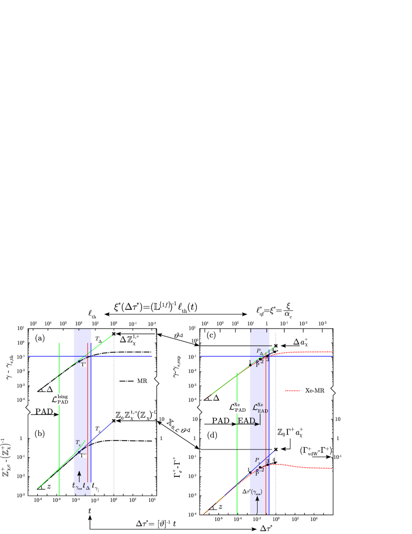
Figure 5: (Color online) a) dot-dashed (black) curve (labeled MR): $\gamma-\gamma_{e,\text{th}}$ as a function of $t$, calculated from the theoretical crossover function of Eq. (43) for susceptibility (log-log scale); (green) line $T_{\Delta}$: limiting singular behavior [see Eq. (134)] within the Ising-like preasymptotic domain of extension $t^{*}<\mathcal{L}_{\text{PAD}}^{\text{Ising}}$ [vertical green line, see Eq. (56)]; curve $T_{\Delta}$ of slope $\Delta$ crossing the vertical line $t=1$ (x): value of the first confluent amplitude of Eq. (55); vertical (blue and pink) lines: $t_{\gamma_{\frac{1}{2}}}$ and $t_{\Delta}$-coordinates for $\gamma_{e,\text{th}}=\gamma_{\frac{1}{2}}$ and $D\left(t_{\Delta}\right)=\Delta_{\frac{1}{2}}$, respectively. b) dot-dashed (black) curve (labeled MR): same as a) for $\left(\mathbb{Z}_{\chi,e}^{+}\right)^{-1}-\left(\mathbb{Z}_{\chi}^{+}\right)^{-1}$ as a function of $t$, calculated from Eq. (43); (green and blue) lines $T_{e}$ and $T_{z}$: logarithmic singularity and power law approximation, [see Eqs. (130) and (131), respectively, and text for detail]; c) and d) dotted (red) curves (labeled Xe-MR): corresponding xenon quantities $\gamma-\gamma_{e}$ and $\Gamma_{e}^{+}-\Gamma^{+}$ as a function of $\Delta\tau^{*}=\left[\vartheta\left(\text{Xe}\right)\right]^{-1}t$; points P and 1 to 4 : $pVT$ results (see Ref. Garrabos2006khiT for detail) given in Table 4 (see also Figure 4); (green and blue) lines $P_{\Delta}$ and $P_{z}$: xenon counterpart of the theoretical (green and blue) lines $T_{\Delta}$ and $T_{z}$. x at $t=\Delta\tau^{*}=1$ : point-to-point transformations between first confluent amplitudes $\mathbb{Z}_{\chi}^{1,+}$ and $a_{\chi}^{+}$ (upper arrow) and between leading amplitudes $\left(\mathbb{Z}_{\chi}^{+}\right)^{-1}$ and $\Gamma^{+}$ (lower arrow).

The following compares these theoretical predictions to the $\gamma_{e,pVT}$ and $\Gamma_{e,pVT}^{+}$ values obtained from $pVT$ measurements Beattie1951 ; Weinberger1952 ; Habgood1954 ; Michels1954 ; Rabinovich1973 (see also details in Ref. Garrabos2006khiT ). We recall that the $pVT$ measurements were performed at finite distance to the critical point, such that the $\kappa_{T,pVT}^{*}$ data obtained from $pVT$ data can be fitted by an effective power law

$$\kappa_{T,pVT}^{*}=\Gamma_{e,pVT}^{+}\left(\Delta\tau^{*}\right)^{-\gamma_{e,pVT}}$$ (123)

only valid in a restricted temperature range defined by $\Delta\tau_{\text{min}}^{*}\leq\Delta\tau^{*}\leq\Delta\tau_{\text{max}}^{*}$. The measured (exponent and amplitude) parameters $\left\{\gamma_{e,pVT};\Gamma_{e,pVT}^{+}\right\}$ are then associated to the temperature range $\left\{\Delta\tau_{\text{min}}^{*};\Delta\tau_{\text{max}}^{*}\right\}$ of central value $\left\langle\Delta\tau_{e,pVT}^{*}\right\rangle=\sqrt{\Delta\tau_{\text{min}}^{*}\Delta\tau_{\text{max}}^{*}}$ (in log scale) located beyond the Ising like preasymptotic domain. Therefore, we can represent these results by points of respective coordinates $\left\{\gamma_{e,pVT};\Gamma_{e,pVT}^{+}\right\}$, $\left\{\gamma_{e,pVT};\left\langle\Delta\tau_{pVT}^{*}\right\rangle\right\}$ and $\left\{\Gamma_{e,pVT}^{+};\left\langle\Delta\tau_{pVT}^{*}\right\rangle\right\}$ in each appropriate binary diagram.

The four points (labeled $1$ to $4$) illustrated in Figs. 4, 5c and 5d, correspond to the xenon results reported on lines labeled $1$ to $4$, respectively, of Table 4. The points labeled $1$ and $2$ follow the general trend of the theoretical curves. This result confirms that, in spite of a large correlated error-bar in the adjustable exponent and amplitude parameters, the variations of their respective central values agree with a two-parameter description within the “Ising-like” side of the crossover domain where $\gamma>\gamma_{e,pVT}>1.17$ . However, the point labeled $3$, and more significantly the point labeled $4$, show that the $pVT$ experimental results are not in agreement with the mean-field behavior predicted by the crossover function within the “mean-field-like” side where $\gamma_{\frac{1}{2}}\gtrsim\gamma_{e,pVT}>\gamma_{\text{MF}}$. The failure of the classical corresponding state theory is also illustrated by the point labeled $5$ in Fig. 4, which corresponds to the result obtained from the van der Waals equation of state [see the line labeled $5\left(\text{vdW})\right)$ in Table 4].

To translate the $\mathcal{L}_{\text{EAD}}^{+,\left\{1f\right\}}$- master value [Eq. (111)] in a $\gamma_{\mathcal{L}}$- master value which delimits the effective range of the extended asymptotic domain in Fig. 4, one needs to consider the upper horizontal axis of Figs. 5c and 5d which measures the master correlation length $\xi^{*}=\frac{\xi}{\alpha_{c}\left(\text{Xe}\right)}$ [i.e. the dimensionless ratio which compares the size of the critical fluctuation to the actual range of the microscopic interaction, with $\Lambda_{qe}^{*}\left(\text{Xe}\right)=1$ in xenon case]. As a matter of fact, the value $\mathcal{L}_{\text{EAD}}^{\text{Xe}}\approx 2\times 10^{-2}$ corresponds to the value $\frac{\mathcal{L}_{\text{EAD}}^{+,\left\{1f\right\}}}{Y_{c}\left(\text{Xe}\right)}$ where $\xi^{*}\approx 3$. Therefore, the associated local value is $\gamma_{\mathcal{L}}\approx 1.16-1.17$. This value descriminates the “non Ising-like” range $\gamma_{e}<\gamma_{\mathcal{L}}$ (including the value $\gamma_{\frac{1}{2}}=\frac{\gamma+\gamma_{\text{MF}}}{2}\approx 1.12$) where the effective classical-to-critical crossover for xenon is no longer accounted for by the theoretical crossover function, as shown in Fig. 4 where it is observed an increasing difference between the curves labeled Xe-MR and the dotted curve labeled Xe-exp when $\gamma_{e}\rightarrow\gamma_{\text{MF}}=1$.

Accounting for an extended (Ising-like) asymptotic domain defined by $\gamma_{e}<\gamma_{\mathcal{L}}$, we are also able to revisit the results previously obtained using an universal scaled form of the equation of state with “universal” values of the exponents significantly different to the “Ising” ones. As a typical example, the xenon results obtained from the restricted linear model of a parametric equation of state with $\gamma_{\text{eos}}=1.19$ [see the line labeled $P\left(\text{eos}\right)$ in Table 4] are in excellent agreement with the theoretical crossover function, as illustrated by the point labeled P in Fig. 4. Moreover, using as a $\Delta\tau^{*}$-coordinate the theoretical value $\Delta\tau_{\text{th}}^{*}\left(\gamma_{\text{eos}}\right)=1.135\times 10^{-2}$ [Eq. (119)], we can show that these results are also well accounted for in the theoretical temperature dependence (see the corresponding points labeled P’ and P” in Figs. 5c and 5d, respectively). Such results confirm that two xenon-parameters involved in an universal form of the equation of state can be used as Ising-like characteristic factors to be related to the two scale factors $Y_{c}$ and $Z_{c}$, as illustrated in the next Section for the case of the linear parametric equation of state.

B.2 Master crossover provided by a restricted linear model of a parametric equation of state

In the seventies, first analyses of the two-scale factor universality for one-component fluids used effective scaled forms of the equation of state (eos) to fit the $pVT$ data measured at finite distance to the critical point (for detail see Refs. Green1967 ; Levelt1974 ; Levelt1975 ; Levelt1976 ; Levelt1978 ; Levelt1981 ; Linearmodelparameter ; Vicentini1969 ). Such a thermodynamic approach of universality was based on a limited number of characteristic parameters for each pure fluid, using effective universal values for the critical exponents. We limit the present purpose to the well-known restricted linear model of the parametric equation of state Linearmodelparameter , with application to several different fluids Levelt1975 . The two main interests for such a choice are the following:

i) The effective thermodynamic exponents have been precisely fixed at (non Ising) values of $\gamma_{\text{eos}}=1.190$, $\beta_{\text{eos}}=0.355$, $\alpha_{\text{eos}}=0.100$ (the subscript eos recalls the origin of these effective values). As shown in Fig. 4, the value $\gamma_{\text{eos}}=1.190$ is precisely within the selected $\gamma_{e}$ range beyond the Ising-like preasymptotic domain, but well inside the extended asymptotic domain $\gamma_{e}<\gamma_{\mathcal{L}}$, which corresponds to $\Delta\tau^{*}\lesssim\mathcal{L}_{\text{EAD}}^{\text{Xe}}$;

ii) The effective values of the thermodynamic amplitude $\Gamma_{\text{eos}}^{+}$ [see below Eq. (124)] of the isothermal compressibility were then obtained only using two adjustable (fluid dependent) parameters (namely $k$ and $a$), which are the two characteristic parameters involved in the scaled equation of state. As shown in Fig. 4, “equivalent” values of $\Gamma_{e}^{+}\left(\gamma_{\text{eos}}\right)$ at $\gamma_{\text{eos}}=1.190$ can be simultaneously obtained by a scale transformation between the point P (on the physical curve) and the point M (on the master curve) which also involves only two characteristic parameters (namely $Y_{c}$ and $Z_{c}$) [admitting that the parameter $\Lambda_{qe}^{*}$ which accounts for quantum effects is known].

Therefore, both in quantity (two), and in nature (Ising like), the fluid dependent parameters $k$ and $a$ appear “equivalent” to $Y_{c}$ and $Z_{c}$, except the noticeable distinction of their respective determination, outside the Ising like preasymptotic domain for the $\left\{k;a\right\}$ pair, asymptotically close to the critical point for the $\left\{Y_{c};Z_{c}\right\}$ pair.

Now we compare the respective values of $\Gamma_{\text{eos}}^{+}$ and $\Gamma_{e}^{+}\left(\gamma_{\text{eos}}\right)$ for twelve selected fluids. From the linear model of the parametric equation of state, Eq. (123) can be rewritten as

$$\kappa_{T}^{*}=\Gamma_{\text{eos}}^{+}\left(\Delta\tau^{*}\right)^{-\gamma_{\text{eos}}}$$ (124)

where $\Gamma_{\text{eos}}^{+}$ is related to the characteristic parameters $k$ and $a$ as follows

$$\Gamma_{\text{eos}}^{+}=\frac{k}{a}$$ (125)

Considering then the restricted form of the linear model such as analyzed in Ref. Levelt1975 , $k$ can be estimated from the relation

$$k=\left(\frac{x_{0}}{b_{\text{SLH}}^{2}-1}\right)^{-\beta_{\text{eos}}}$$ (126)

where $b_{\text{SLH}}^{2}=1.3908$ is an universal quantity while $x_{0}$ is a fluid-dependent parameter related to the value of the effective amplitude of the coexistence curve (associated to the value $\beta_{\text{eos}}=0.355$ of the effective exponent). The values of $x_{0}$ and $a$ can be found in Ref. Levelt1975 . They are reported with the corresponding $k$ values in Table 5 (columns $2$ to $4$, respectively) for the selected twelve fluids (column 1). The related values of $\Gamma_{\text{eos}}^{+}$ obtained by using Eq. (125) are given in Table 5 (column $5$).

Fluid	$x_{0}$	$a$	$k$	$\Gamma_{\text{eos}}^{+}$	$Y_{c}$	$Z_{c}$	$\Gamma_{e}^{+}\left(\gamma_{\text{eos}}\right)$	$\Delta\tau^{*}\left(\gamma_{\text{eos}}\right)$	$r\%(\Gamma_{e}^{+})$
	Levelt1975	Levelt1975	Eq. (126)	Eq. (125)			Eq. (127)	Eq. (129)
3He(∗)	$0.489$	$4.63$	$0.9235$	$0.1995$	$2.3984$	$0.30129$	$0.20003$(∗)	$2.326\,10^{-2}$	$-0.283$
Ar	$0.183$	$16.5$	$1.309$	$0.07934$	$4.3288$	$0.2896$	$0.09284$	$1.289\,10^{-2}$	$-14.5$
Kr	$0.183$	$16.5$	$1.309$	$0.07934$	$4.9437$	$0.2913$	$0.07887$	$1.128\,10^{-2}$	$0.6$
Xe	$0.183$	$16.5$	$1.309$	$0.07934$	$4.9137$	$0.2860$	$0.08084$	$1.135\,10^{-2}$	$-1.86$
O2	$0.183$	$15.6$	$1.309$	$0.08392$	$4.9864$	$0.28797$	$0.07890$	$1.119\,10^{-2}$	$6.36$
N2	$0.164$	$18.2$	$1.361$	$0.07478$	$5.3701$	$0.28887$	$0.07201$	$1.039\,10^{-2}$	$3.84$
CH4	$0.164$	$17.0$	$1.361$	$0.08006$	$4.9838$	$0.28678$	$0.07928$	$1.119\,10^{-2}$	$0.99$
C2H4	$0.166$	$17.5$	$1.355$	$0.07744$	$5.3487$	$0.2813$	$0.07431$	$1.043\,10^{-2}$	$4.22$
CO2	$0.141$	$21.8$	$1.436$	$0.06587$	$6.0104$	$0.27438$	$0.06631$	$0.928\,10^{-2}$	$0.653$
NH3	$0.109$	$21.4$	$1.361$	$0.07353$	$6.3019$	$0.24294$	$0.07079$	$0.885\,10^{-2}$	$3.88$
H2O	$0.100$	$22.3$	$1.622$	$0.07275$	$6.8552$	$0.22912$	$0.0679$	$0.814\,10^{-2}$	$7.14$
D2O	$0.100$	$22.3$	$1.622$	$0.07275$	$7.0728$	$0.22783$	$0.0658$	$0.799\,10^{-2}$	$10.6$

Table 5: Two-parameter universality of the effective amplitude of the isothermal compressibility estimated from the linear model of a parametric equation of state and the master modification of the theoretical function.

The unequivocal scale transformation between the points P and M is given by the relation (see Fig. 4)

$$\Gamma_{e}^{+}(\gamma_{\text{eos}})=\mathbb{\mathcal{Z}}_{\chi,e}^{+}\left(\gamma_{\text{eos}}\right)\frac{\Lambda_{qe}^{*}\left(Y_{c}\right)^{-\gamma_{eos}}}{Z_{c}}$$ (127)

where $\mathbb{\mathcal{Z}}_{\chi,e}^{+}\left(\gamma_{\text{eos}}\right)$ is the effective master amplitude for the $\mathcal{T}^{*}\left(\gamma_{e,1f}\right)$-value satisfying the condition $\gamma_{e,1f}=\gamma_{\text{eos}}=1.19$. For practical use of Eq. (127), the crucial advantage is given by the uniquivocal scale transformation between the points T (on the theoretical curve) and M (on the master curve) illustrated in Fig. 4. That provides immediately $\mathbb{\mathcal{Z}}_{\chi,e}^{+}\left(\gamma_{\text{eos}}\right)=\mathbb{\mathcal{\mathbb{Z}}}_{\chi,e}^{+}\left(\gamma_{\text{eos}}\right)\left[\mathbb{Z}_{\chi}^{\left\{1f\right\}}\left(\Theta^{\left\{1f\right\}}\right)^{\gamma_{\text{eos}}}\right]^{-1}$ and $\mathcal{T}^{*}\left(\gamma_{\text{eos}}\right)=t\left(\gamma_{\text{eos}}\right)\left(\Theta^{\left\{1f\right\}}\right)^{-1}$. Using Eqs. (117) and (118), the theoretical function $\chi_{\text{th}}\left(t\right)$ leads to the values $t\left(\gamma_{\text{eos}}\right)=2.392\times 10^{-4}$ and $\mathbb{\mathcal{\mathbb{Z}}}_{\chi,e}^{+}\left(\gamma_{\text{eos}}\right)=0.456414$ related to coordinates of the points labeled T’ and T” in Figs. 5a and 5b, respectively. Using the numerical values of $\mathbb{Z}_{\chi}^{\left\{1f\right\}}$ and $\Theta^{\left\{1f\right\}}$ given in Table 2, we obtain $\mathcal{T}^{*}\left(\gamma_{\text{eos}}\right)=5.579\times 10^{-2}$ and $\mathbb{\mathcal{Z}}_{\chi,e}^{+}\left(\gamma_{\text{eos}}\right)=0.15374$. Subsidiarily, in Fig. 1c, we note that the master curve $\chi_{\text{qf}}^{*}\left(\mathcal{T}^{*}\right)$ of Eq. (84) has a tangent curve of slope $-\gamma_{\text{eos}}$ at the point M of $\mathcal{T}^{*}\left(\gamma_{\text{eos}}\right)$-coordinate which corresponds to the effective power law

$$\mathbb{\mathcal{X}}_{\text{eos}}^{+}\left(\mathcal{T}^{*}\right)=0.15374\left(\mathcal{T}^{*}\right)^{-1.19}$$ (128)

The values of $Y_{c}$ and $Z_{c}$ for the selected fluids are reported in Table 5 (columns $6$ and $7$, respectively). The estimated values of $\Gamma_{e}^{+}(\gamma_{\text{eos}})$ using Eq. (127) are given in Table 5 (column $8$). Each physical curve $\kappa_{T}^{*}\left(\Delta\tau^{*}\right)$ of Eq. (66) have a tangent curve of slope $-\gamma_{\text{eos}}$ at the point of $\Delta\tau^{*}$-coordinate:

$$\Delta\tau^{*}\left(\gamma_{\text{eos}}\right)=\frac{\mathcal{T}^{*}\left(\gamma_{\text{eos}}\right)}{Y_{c}}$$ (129)

(see column $9$ of Table 5), which corresponds to the effective power law $\Gamma_{e}^{+}\left(\Delta\tau^{*}\right)=\Gamma_{e}^{+}(\gamma_{\text{eos}})\left(\Delta\tau^{*}\right)^{-\gamma_{\text{eos}}}$ .

The residuals $r\%(\Gamma_{e}^{+})=100\left(\frac{\Gamma_{\text{eos}}^{+}}{\Gamma_{e}^{+}(\gamma_{\text{e}\text{os}})}-1\right)$ (see column $10$, Table 5), generally lower than the typical experimental uncertainty estimated to $10\%$, confirm that the universal features observed beyond the Ising-like preasymptotic domain but within the Ising-like extended asymptotic domain, i.e., $\Delta\tau^{*}\lesssim\frac{t_{\text{EAD}}^{+}}{\vartheta}=\frac{\mathcal{L}_{\text{EAD}}^{+,\left\{1f\right\}}}{Y_{c}}=\mathcal{L}_{\text{EAD}}^{f}$ with $t_{\text{EAD}}^{+}=\Theta^{\left\{1f\right\}}\mathcal{L}_{\text{EAD}}^{+,\left\{1f\right\}}$ and $\mathcal{L}_{\text{EAD}}^{+,\left\{1f\right\}}\simeq 0.07-0.1$, are well-characterized by the two critical scale factors $Y_{c}$ and $Z_{c}$ of each fluid $f$.

B.3 “Universal” approximation of the logarithmic singularity of effective amplitudes

Another practical application of the point to point transformations given in Fig. 4 can be obtained focusing our attention on the logarithmic singularity of any first derivative $\left(\frac{\partial\mathbb{Z}_{P,e}^{+}}{\partial e_{P,e}}\right)_{e_{P,e}\rightarrow e_{P}}$ close to the Ising-like critical point, for any effective amplitude power law $\mathbb{Z}_{P,e}^{+}\left(t\right)=\frac{F_{P}\left(t\right)}{t^{-e_{P,e}}}$ estimated from any crossover function $F_{P}\left(t\right)$ given in Ref. Garrabos2006gb (with $e_{P,e}\left(t\right)=-\frac{\partial Ln\left[F_{P}\left(t\right)\right]}{\partial Lnt}$) (see Refs. Garrabos2006gb ; Garrabos2006khiT for detail). For the susceptibility case, the logarithmic singularity of $\left(\frac{\partial\mathbb{Z}_{\chi,e}^{+}}{\partial\gamma_{e,th}}\right)_{\gamma_{e,th}\rightarrow\gamma}$ extrapolated beyond the Ising-like preasymptotic domain is illustrated by the curves labeled $a_{T}$, $a_{M}$, and $a_{P}$ in Fig. 4. For better evaluation within the preasymptotic domain, the related amplitude singularity in terms of the thermal field dependence is given in Fig. 5b for example by the curve $T_{e}$ of equation

$$\begin{array}[]{cl}\mathbb{Z}_{\chi,e}^{+}-\left(\mathbb{Z}_{\chi}^{+}\right)^{-1}=&\left(\mathbb{Z}_{\chi}^{+}\right)^{-1}\mathbb{Z}_{\chi}^{1,+}t^{\Delta\mathbb{Z}_{\chi}^{1,+}t^{\Delta}}\\ &\times\left[1-log\left(t^{\Delta}\right)\right]t^{\Delta}\end{array}$$ (130)

We can approximate Eq. (130) by the following “universal” power law

$$\mathbb{Z}_{\chi,e}^{+}-\left(\mathbb{Z}_{\chi}^{+}\right)^{-1}=\mathbb{Z}_{0}\left(\mathbb{Z}_{\chi}^{+}\right)^{-1}\mathbb{Z}_{\chi}^{1,+}t^{z}$$ (131)

where $\mathbb{Z}_{0}=3.7\pm 0.1$ and $z=0.45\pm 0.035$ are independent of the property and the domain. The exponent condition $z<\Delta$, leading to the $\frac{z}{\Delta}=1-u<1$, is conform to the logarithmic singularity of the first derivative $\left(\frac{\partial\mathbb{Z}_{\chi,e}^{+}}{\partial\gamma_{e,\text{th}}}\right)_{\gamma_{e,\text{th}}\rightarrow\gamma}$ here approximated by a power law $\left(\frac{\partial\mathbb{Z}_{\chi,e}^{+}}{\partial\gamma_{e,\text{th}}}\right)_{\gamma_{e,\text{th}}\rightarrow\gamma}\propto\left(\gamma-\gamma_{e,\text{th}}\right)^{-u}$. For practical use, we arbitrarily choose $u=\alpha$, leading to define $z=\Delta\left(1-\alpha\right)$. The validity of this approximation is illustrated by the curve $T_{z}$ in Figure 5b.

Correspondingly, in Figure 5d, the physical asymptotic representation of $\Gamma_{e}^{+}-\Gamma^{+}$ is now approximated by the curve $P_{z}$ of asymptotic equation

$$\begin{array}[]{cl}\Gamma_{e}^{+}-\Gamma^{+}&=\mathbb{Z}_{0}\Gamma^{+}a_{\chi}^{+}\left(\Delta\tau^{*}\right)^{z}\\ &=\mathbb{X}_{0,\mathcal{L}}\mathbb{Z}_{0}\mathbb{Z}_{\chi}^{1,+}\left(\mathbb{Z}_{\mathcal{X}}^{+}\right)^{-1}\vartheta^{\Delta}\left(\Delta\tau^{*}\right)^{z}\end{array}$$ (132)

Using Eqs. (131) and (132) at $t=\Delta\tau^{*}=1$, we obtain

$$\Gamma_{e}^{+}\left(1\right)-\Gamma^{+}=\mathbb{X}_{0,\mathcal{L}}^{*}\vartheta^{\Delta}\left[\mathbb{Z}_{\chi,e}^{+}\left(1\right)-\left(\mathbb{Z}_{\chi}^{+}\right)^{-1}\right]$$ (133)

The point to point “universal” transformation which approximates the logarithmic singularity is then illustrated by the two correlated points (symbol x) at $t=\Delta\tau^{*}=1$, in Figures 5b and 5d, respectively. As expected from Figure 4, this transformation is given by the product $\mathbb{X}_{0,\mathcal{L}}^{*}\vartheta^{\Delta}$.

Obviously, to close the asymptotic behavior within the Ising-like preasymtotic domain we can also consider the respective asymptotic curves labeled $T_{\Delta}$ and $P_{\Delta}$ in Figs. 5a and 5c of equations

$$\gamma-\gamma_{e,\text{th}}=\Delta\,\mathbb{Z}_{\chi}^{1,+}t^{\Delta}$$ (134)

$$\gamma-\gamma_{e,\text{exp}}=\Delta\,a_{\chi}^{+}\left(\Delta\tau\right)^{\Delta}$$ (135)

Here, the point to point transformation at $t=\Delta\tau^{*}=1$ (symbol x), is given by the scale factor universal power law $\vartheta^{\Delta}$.

The above approximation of the logarithmic singularity has a practical importance for better analysis of experimental data when the value $\gamma_{e}$ is found in the range $\gamma_{e}=1.21-1.24$, i.e. a value which “approaches” the theoretical Ising value. As a typical example we use the value $\gamma_{e,pVT}=1.211\pm 0.025$ obtained by Levelt-Sengers et al Levelt1975 from their analysis of the $pVT$ measurements of Habgood and Schneider Habgood1954 in the temperature range $0.2\,K\leq T-T_{c}\leq 1.8\,K$ , i. e. $\Delta\tau_{\text{min}}^{*}=6.9\times 10^{-4}$, $\Delta\tau_{\text{max}}^{*}=6.2\times 10^{-3}$ and $\left\langle\Delta\tau_{pVT}^{*}\right\rangle=2.07\times 10^{-3}$ [see line $\#1$, column $4$, Table IV]. This result is then centered near to the Ising-like borderline of the gray paint domain previously analyzed. As evidenced by the matching of the corresponding points labeled $1$ with the curves $P_{\Delta}$ and $P_{z}$ in Figs. 5c and 5d, such a result also appears correctly accounted for using the above approximation. Therefore, using Eqs. (135) and (132), we can easily calculate the two values of the true confluent and leading amplitudes of the two-term Wegner expansion from the following equations

$$\left.a_{\chi}^{+}\right|_{pVT} =\frac{\gamma-\gamma_{e,pVT}}{\Delta\left\langle\Delta\tau_{pVT}^{*}\right\rangle^{\Delta}}$$

$$=1.26666$$

$$\left.\Gamma^{+}\right|_{pVT} =\frac{\Gamma_{e,pVT}^{+}}{1+\frac{\mathbb{Z}_{0}}{\Delta}\left(\gamma-\gamma_{e,pVT}\right)\left\langle\Delta\tau_{pVT}^{*}\right\rangle^{z-\Delta}}$$

$$=0.057355$$

These above values are in excellent agreement with the estimated ones $a_{\chi}^{+}=1.23397$ and $\Gamma^{+}=0.05782$1 Garrabos2006khiT from application of the scale dilatation method. In Eq. (B.3), we note the practical importance of the prefactor $\mathbb{Z}_{0}$.

In conclusion, using Figs 4 and 5, we have explicitely demonstrated that the two dimensionless scale factors $Y_{c}$ and $Z_{c}$, (or alternatively but equivalently $\vartheta_{\mathcal{L}}\left(\equiv\vartheta\right)$ and $\mathbb{X}_{0,\mathcal{L}}^{*}$), which characterize each one-component fluid $f$ belonging to $\left\{1f\right\}$-subclass, can be used to calculate the isothermal compressibility over a Ising-like extended asymptotic domain $\Delta\tau^{*}\lesssim\mathcal{L}_{\text{EAD}}^{f}$.

References

• (1) see for example Zinn Justin, Euclidean Field Theory and Critical Phenomena , $4^{th}$ ed. (Clarendon, Oxford, 2002).
• (2) see, for example, A. Pelissetto and E. Vicari, Phys. Rept. 368, 549 (2002), and references therein.
• (3) K. G. Wilson and M. E. Fisher, Phys. Rev. Lett. 28, 240 (1972).
• (4) K. G. Wilson and J. Kogut, Phys. Rep. 12 C, 75 (1974).
• (5) A. Pelissetto, P. Rossi, and E. Vicari, Phys. Rev. E 58, 7146 (1998).
• (6) For a review see for example, M. A. Anisimov and J. V. Sengers, in Equations of State for Fluids and Fluid Mixtures, edited by J. V. Sengers, R. F. Kayser, C. J. Peters, and H. J. White, Jr. (Elsevier, Amsterdam, UK, 2000), Part I, pp. 381-434, and references therein.
• (7) C. Bagnuls and C. Bervillier, J. Phys. (Paris) Lett., 45, L-95 (1984).
• (8) C. Bagnuls and C. Bervillier, Phys. Rev. B 32, 7209 (1985);
• (9) C. Bagnuls, C. Bervillier, D. I. Meiron, and B. G. Nickel, Phys. Rev. B 35, 3585 (1987); 65, 149901(E) (2002).
• (10) C. Bagnuls and C. Bervillier, Phys. Rev. E 65, 066132 (2002).
• (11) Another equivalent renormalization scheme (called minimal) used for example by Dohm and co-workers is not directly considered here; see V. Dohm, Z. Phys. B: Condens. Matter 60, 61 (1985); R. Schloms and V. Dohm, Europhys. Lett. 3, 413 (1987); Nucl. Phys. B 328, 639 (1989); Phys. Rev. B 42, 6142 (1990); H. J. Krause, R. Schloms and V. Dohm, Z. Phys. B: Condens. Matter 79, 287 (1990); see also below Refs. Zhong2003 ; Zhong2004 .
• (12) C. Bagnuls, C. Bervillier, and Y. Garrabos, J. Phys. (Paris) Lett. 45, L-127 (1984).
• (13) Y. Garrabos and C. Bervillier, Phys. Rev. E 74, 021113 (2006).
• (14) R. Guida and J. Zinn-Justin, J. Phys. A: Math. Gen. 31, 8103 (1998).
• (15) F. J. Wegner, Phys Rev. B 5, 4529 (1972).
• (16) J. M. H. Levelt Sengers and J. V. Sengers, in Progress in Liquid Physics, edited by C. A. Croxton (John Wiley & Sons, New York, 1978) pp. 103.
• (17) V. Privman, P. C. Hohenberg, and A. Aharony, in Phase Transitions and Critical Phenomena, edited by C. Domb and J. B. Lebowitz (Academic Press, New York, 1991), Vol. 14.
• (18) J. M. H. Levelt-Sengers and J. V. Sengers, in Perspectives in Statistical Physics, edited by H. J. Raveché (North-Holland Publishing Company, 1981), pp. 241-271.
• (19) E. Luijten and K. Binder, Europhys. Lett. 47, 311 (1999).
• (20) E. Luijten and H. Meyer, Phys. Rev. E 62, 3257 (2000).
• (21) M. H. Müser and E. Luijten, J. Chem. Phys. 116, 1621 (2002).
• (22) I. Hahn, F. Zhong, M. Barmatz, R. Haussmann, and J. Rudnick, Phys. Rev. E 63, 055104(R) (2001).
• (23) F. Zhong and M. Barmatz, Phys. Rev. E 70, 066105 (2004).
• (24) F. Zhong, M. Barmatz, and I. Hahn, Phys. Rev. E 67, 021106 (2003).
• (25) J. S. Kouvel and M. E. Fisher, Phys. Rev. 136, A 1626 (1964).
• (26) Z. Y. Chen, P. C. Albright, and J. V. Sengers, Phys. Rev. A 41, 3161 (1990).
• (27) Z. Y. Chen, A. Abbaci, S. Tang, and J. V. Sengers, Phys. Rev. A 42, 4470 (1990).
• (28) M. A. Anisimov, S. B. Kiselev, J. V. Sengers, and S. Tang, Physica A 188, 487 (1992).
• (29) M. A. Anisimov, A. Povodyrev, V. Kulikov, and J. V. Sengers, Phys. Rev. Lett. 75, 3146 (1995).
• (30) V. A. Agayan, M. A. Anisimov, and J. V. Sengers, Phys. Rev. E 64, 026125 (2001).
• (31) J. O. Hirschfelder, C. F. Curtiss, and R. B. Bird, Molecular Theory of Gases and Liquids (Wiley, New York, 1954).
• (32) C. Bagnuls and C. Bervillier, Phys. Rev. Lett. 76, 4094 (1996).
• (33) M. Campostrini, A. Pelissetto, P. Rossi, and E. Vicari, Phys. Rev. E 65, 066127 (2002).
• (34) E. Luijten, H. W. J. Blöte, and K. Binder, Phys. Rev. Lett. 79, 451 (1997): Phys. Rev. E 54, 4626 (1996); 56, 6540 (1997).
• (35) Y. Garrabos, Ph.D. thesis, University of Paris VI (1982).
• (36) Y. Garrabos, J. Phys. (France) 46, 281 (1985) [for an english version see cond-mat/0512347 (2005)].
• (37) Y. Garrabos, J. Phys. (France) 47, 197 (1986).
• (38) Y. Garrabos, Phys. Rev. E 73, 056110 (2006).
• (39) Y. Garrabos, F. Palencia, C. Lecoutre, C. Erkey, and B. Le Neindre, Phys. Rev. E 73, 026125 (2006).
• (40) Y. Garrabos, F. Palencia, C. Lecoutre, D. Brosetta, B. Le Neindre, and C. Erkey, Phys. Rev. E 75, 061112 (2007).
• (41) Y. Garrabos, F. Palencia, C. Lecoutre, D. Brosetta, and B. Le Neindre, preprint (2007); see http:// hal.archives-ouvertes.fr/hal-00162446.
• (42) L. Riedel, Chem. Eng. Tech. 26, 83 (1954).
• (43) See for example, R. Reid., J. M. Prausnitz, B. E. Poling, The properties of gases and liquids, $4^{th}$ edition (McGraw Hill, New York, 1988); J. F. Ely and I. M. F. Marrucho, in Equations of State for Fluids and Fluid Mixtures, edited by J. V. Sengers, R. F. Kayser, C. J. Peters, and H. J. White, Jr. (Elsevier, Amsterdam, UK, 2000), Part I, pp. 289-320; H. W. Xiang, Corresponding-States Principle and Practice (Elsevier, Amsterdam, 2005).
• (44) R. B. Griffiths and J. C. Wheeler, Phys. Rev. A2, 1047 (1970).
• (45) $Z$ takes extremum (minimum) value along the vapor-liquid equilibrium line and continuously decreases as density increases from gas to liquid in coexistence.
• (46) Y. Garrabos, B. Le Neindre, R. Wunenburger, C. Lecoutre-Chabot, and D. Beysens, Int. J. Thermophys. 23, 997 (2002).
• (47) Such a way was only suggested and practically not used in the conclusive discussion given in Ref. Bagnuls1984b , due to the large fitting uncertainty in the $\vartheta_{\mathcal{L}}$ determination, added to the large theoretical uncertainties in the Ising-like asymptotic forms of the crossover functions estimated from the dated development of the massive renormalization scheme.
• (48) Y. Garrabos, C. Lecoutre, and F. Palencia, preprint (2007); see http://hal.archives-ouvertes.fr/hal-00165475.
• (49) H. Güttinger and D. S. Cannell, Phys. Rev. A 24, 3188 (1981).
• (50) see for example, S. B. Kiselev and J. F. Ely, J. Chem. Phys. 119, 8645 (2003).
• (51) J. A. Beattie, R. J. Barriault, and J. S. Brierley, J. Chem. Phys. 19, 1219 (1951); 19, 1222 (1951).
• (52) M. A. Weinberger and W. G. Schneider, Can. J. Chem. 30, 422 (1952); 30, 847 (1952).
• (53) H. W. Habgood and W. G. Schneider, Can. J. Chem. 32, 98 (1954); 32, 164 (1954).
• (54) A. Michels, T. Wassenaar, and P. Louwerse, Physica 20, 99 (1954).
• (55) V. A. Rabinovich, L. A. Tokina, V. M. Berezin, Teplo. Vys. Temp. 11, 64 (1973); V. A. Abovskii and V. A. Rabinovich, Teploenerg. 3, 44-57 (1971); 6, 45-93 (1973).
• (56) M. S. Green, M. Vicentini-Missoni, and J. M. H. Levelt Sengers, Phys. Rev. Lett. 18, 1113 (1967).
• (57) M. Vicentini-Missoni, J. M. H. Levelt Sengers, and M. S. Green, J Res. Natl. Bur. Stand. 73A, 563 (1969).
• (58) J. M; H. Levelt Sengers, Physica 73, 73 (1974).
• (59) J. M. H. Levelt Sengers and J. V. Sengers, Phys. Rev. A 12, 2622 (1975).
• (60) J. M. H. Levelt Sengers, W. L. Greer, and J. V. Sengers, J. Phys. Chem. Ref. Data 5, 1 (1976).
• (61) See Table 4.3.4, p. 144 in Ref. Levelt1978 .