Ergodicity in
Strongly Correlated Systems

Abstract

We present a concise, but systematic, review of the ergodicity issue in strongly correlated systems. After giving a brief historical overview, we analyze the issue within the Green’s function formalism by means of the equations of motion approach. By means of this analysis, we are able to individuate the primary source of non-ergodic dynamics for a generic operator and also to give a recipe to compute unknown quantities characterizing such a behavior within the Composite Operator Method. Finally, we present examples of non-trivial strongly correlated systems where it is possible to find a non-ergodic behavior.

Key words: Ergodicity, Strongly Correlated Systems, Green’s Function Formalism, Equations of Motion Approach, Composite Operator Method

PACS: 05.30.Jp, 75.10.Jm, 71.10.-w

1 Historical Overview

The issue of ergodicity in condensed matter physics is well known since fifties [1]. Given two operators $A$ and $B$, describing physical quantities (e.g., charge, spin, pair densities or currents), one can study the physical response of a system described by a certain Hamiltonian $H$ through the generalized susceptibility

$$\chi_{AB}=\lim_{h\to 0}\frac{\partial\langle A\rangle}{\partial h}$$ (1.1)

where $h$ is an external field entering the Hamiltonian of the system under study in a coupling term of the type $-hB$ and $\langle\cdots\rangle$ stands for the statistical average in some ensemble over the perturbed system. Kubo [1] immediately noticed that the static isolated susceptibility $\chi^{I}(0)$, defined for an isolated system perturbed by an external field turned on adiabatically, and the isothermal susceptibility $\chi^{T}$, defined for a system in thermal equilibrium in presence of a time-independent external field, can be generally different. In particular, Falk [2] has shown that the static isolated susceptibility is just a lower bound for the isothermal one $\chi^{I}(0)\leq\chi^{T}$.

We recall that the static isolated susceptibility $\chi^{I}(0)$, within the linear response theory, is defined through the related retarded Green’s function [1]

$$\chi^{I}(\omega)=-\mathcal{F}\left[\mathrm{i}\,\theta(t_{i}-t_{j})\left\langle\left[A(t_{i}),B(t_{j})\right]\right\rangle_{0}\right]$$ (1.2)

where $\langle\cdots\rangle_{0}$ stands for the statistical average in the microcanonical ensemble (i.e., fixing energy) on the unperturbed system and $\mathcal{F}$ for the Fourier transform.

On the other hand, the isothermal susceptibility $\chi^{T}$ can be computed as

$$\chi^{T}=\int_{0}^{\beta}\langle A(-\mathrm{i}\lambda)B\rangle_{0}\,d\lambda-\beta\langle A\rangle_{0}\langle B\rangle_{0}$$ (1.3)

In fact, starting from the expression of the thermal average in the canonical ensemble (i.e., fixing temperature) $\langle A\rangle$

$$\langle A\rangle=\frac{1}{Z}\operatorname{Tr}\left(Ae^{-\beta(H-hB)}\right)$$ (1.4)

where $\beta=\frac{1}{T}$ and $Z=\operatorname{Tr}\left(e^{-\beta H-hB}\right)$, we can expand $e^{-\beta(H-hB)}$ in powers of $h$ and get

$$e^{-\beta(H-hB)}\approxeq e^{-\beta H}\left(1+h\int_{0}^{\beta}d\lambda e^{\lambda H}Be^{-\lambda H}+O(h^{2})\right)$$ (1.5)

Substituting this expansion into (1.4) and retaining only the first order term in $h$, we get at the numerator

$$\operatorname{Tr}\left(Ae^{-\beta(H-hB)}\right)\approxeq Z_{0}\langle A\rangle_{0}+hZ_{0}\int_{0}^{\beta}d\lambda\langle AB(i\lambda)\rangle_{0}$$ (1.6)

and at the denominator

$$Z\approxeq Z_{0}\left(1+h\beta\langle B\rangle_{0}\right)$$ (1.7)

and by the ratio

$$\langle A\rangle\approxeq\langle A\rangle_{0}+h\int_{0}^{\beta}d\lambda\langle AB(i\lambda)\rangle_{0}-h\beta\langle A\rangle_{0}\langle B\rangle_{0}$$ (1.8)

where $Z_{0}$ denotes the partition function of the unperturbed system. Taking the derivative after (1.1) and exploiting the cyclic property of the trace, we obtain the isothermal susceptibility as in (1.3).

Now, if we rewrite both expressions by means of the general formulas for the retarded Green’s functions and the correlation functions given in the companion article [3] (see Section 3), present in this same issue, we get

$$\chi^{I}(0)=\frac{1}{V}\sum_{\mathbf{k},l}\frac{\sigma^{(l,-1)}(\mathbf{k})}{\omega_{l}(\mathbf{k})}$$ (1.9)

and

$$\chi^{T}=\beta\frac{1}{V}\sum_{\mathbf{k}}\Gamma_{AB}(\mathbf{k})+\frac{1}{V}\sum_{\mathbf{k},l}\frac{\sigma^{(l,-1)}(\mathbf{k})}{\omega_{l}(\mathbf{k})}-\beta\langle A\rangle_{0}\langle B\rangle_{0}$$ (1.10)

where [3, 4] $V$ is proportional to the volume of the system, the sum over $l$ ranges over the number of fields in the chosen basis, $\sigma^{(l)}$ are the spectral density functions, $\omega^{(l)}$ are the poles of the propagator, $\Gamma_{AB}$ is an unknown function appearing in case of poles with zero value.

We can immediately see that the two susceptibilities differ for the following expression

$$\chi^{T}-\chi^{I}(0)=\beta\frac{1}{V}\sum_{\mathbf{k}}\Gamma_{AB}(\mathbf{k})-\beta\langle A\rangle_{0}\langle B\rangle_{0}$$ (1.11)

Now, one can check that rewriting the expression $\lim_{t\to\infty}\langle AB(t)\rangle$ by means of the general formula for the correlation functions given in the companion article [3] (see Section 3), present in this same issue, we just get

$$\lim_{t\to\infty}\langle AB(t)\rangle=\frac{1}{V}\sum_{\mathbf{k}}\Gamma_{AB}(\mathbf{k})$$ (1.12)

and, accordingly, the difference at the r.h.s. of (1.11) is just what enters Khintchin’s theorem [5]: a dynamics is ergodic (i.e., phase space equilibrium averages are equal to ensemble microcanical averages, which are much easier to compute)

$$\langle AB\rangle=\int_{0}^{\infty}dt\overline{AB(t)}$$ (1.13)

if an only if

$$\lim_{t\to\infty}\langle AB(t)\rangle=\langle A\rangle\langle B\rangle$$ (1.14)

In other words a dynamic is ergodic if correlations attenuate in time. In particular, for $B\equiv A$, the dynamics of $A$ is ergodic if, during its time evolution, it has non-zero matrix elements only between states within a zero-volume region of the phase space of the system [6].

It is clear now the link between ergodicity and response theory: the two definitions of susceptibility differ when the dynamics of the system is not ergodic. Two little, but important, notices: finite systems are not ergodic by definition, just because of the inequivalence of the ensembles; non-ergodicity at zero temperature is just the result of a degeneracy in the ground state.

Several years later it was shown [7, 8] that the difference between the two definitions of susceptibility is related to the zero-frequency anomaly exhibited by bosonic correlation functions: the presence of undetermined constants in the bosonic correlation functions. This is exactly what the relations derived above and the results of the companion article [3] predict establishing a definite link between the ergodicity of the dynamics and the Green’s function formalism. It was first put in evidence in [9] and then studied by many other authors [10, 11, 7, 8, 6, 12, 13, 14, 15, 16]. There is a general believe that this problem is of academic interest and in the last years no much attention has been dedicated to it. The main reason is that the response functions, the experimentally observed quantities, are given by retarded bosonic Green’s function which formally do not depend on the such undetermined constants, which are, therefore, considered of no physical interest. The general attitude [1, 10] is to believe that in macroscopic real systems at equilibrium at a temperature $T$, the fluctuations are very small and the interaction between the system and the reservoir would introduce an irreversible relaxation and decouple the correlation functions. Then, as suggested in [10], these constants should be always determined by requiring the ergodicity. This procedure is some how an artifice and may lead to serious problems because it might break the internal self-consistency of the entire formulation. As remarked in [10], the zero-frequency anomaly is a manifestation of the difficulty in extracting irreversible behavior from the statistical mechanics. This is true, but as long as we use the scheme of statistical mechanics we must be careful in doing self-consistent calculations. Breaking the self-consistency might bring to serious errors.

According to the well-known relations existing between casual ($C$), retarded ($R$) Green’s functions and correlation functions

$$\Re[G^{R}({\bf k},\omega)]=\Re[G^{C}({\bf k},\omega)]$$ (1.15)

$$\Im[G^{R}({\bf k},\omega)]=\tanh\left({{{\beta\omega}\over 2}}\right)\Im[G^{C}({\bf k},\omega)]$$ (1.16)

$$C({\bf k},\omega)=-\left[{1+\tanh\left({{{\beta\omega}\over 2}}\right)}\right]\Im[G^{C}({\bf k},\omega)]$$ (1.17)

the zero-frequency excitations do not contribute explicitly to the imaginary part of the retarded Green’s functions and, consequently, $\Gamma$ does not explicitly appear in the expressions of susceptibilities. At any rate, susceptibilities retain an implicit dependence on $\Gamma$ through the matrix elements. Then, the right procedure to compute both correlation functions and susceptibilities is clearly the one that starts from the causal Green’s function, which is the only Green’s function that explicitly depends on $\Gamma$. It is worth noticing that the value of $\Gamma$ dramatically affects the values of directly measurable quantities (e.g., compressibility, specific heat, magnetic susceptibility, …) through the values of correlation functions and susceptibilities. According to this, whenever it is possible, $\Gamma$ should be exactly calculated case by case.

If we do not have access to the complete set of eigenstates and eigenvalues of the system, which is the rule in the most interesting cases, we have to compute correlation functions and susceptibilities within some, often approximated, analytical framework. Now, since no analytical tool can easily determine $\Gamma$ (e.g., the equations of motion cannot be used to fix $\Gamma$ as it is constant in time), one usually assumes the ergodicity of the dynamics of $\psi$ and simply substitutes $\Gamma$ by its ergodic value (i.e., by the r.h.s. of (1.14)):

$$\Gamma^{erg}({\bf i},{\bf j})=\langle\psi({\bf i})\rangle\langle\psi^{\dagger}({\bf j})\rangle.$$ (1.18)

Unfortunately, this procedure cannot be justified a priori (i.e., without computing $\Gamma$ through its definition (2.62)) by absolutely no means. The existence of just one integral of motion and, more generally, of any operator that has a diagonal part with respect to the Hamiltonian [6] (i.e. by any operator that has a diagonal entries whenever written in the basis of eigenstates of the Hamiltonian) divides the phase space into separate subspaces not connected by the dynamics. This latter, in turn, becomes non ergodic: time averages give different results with respect to ensemble averages. This latter consideration also clarifies why the ergodic nature of the dynamics of an operator mainly depends on the Hamiltonian it is subject to.

It is really remarkable that $\Gamma$ is directly related to relevant measurable quantities such as compressibility and specific heat trough the dissipation-fluctuation theorem. For instance, we recall the formula that relates the compressibility to the total particle number fluctuations

$$\kappa=\beta\frac{V}{N^{2}}\left[\langle\hat{N}^{2}\rangle-N^{2}\right]$$ (1.19)

where $\hat{N}$ is the total particle number operator, $N$ is its average and $V$ is proportional to the volume of the system. We see that a compressibility different from zero requires the non-ergodicity of the system with respect to total particle number operator. According to this, in the case of infinite systems too the correct determination of $\Gamma$ cannot be considered as an irrelevant issue (e.g., (1.19) holds in the thermodynamic limit too).

In the next section, we provide some examples of violation of the ergodic condition (1.14). It is necessary pointing out, in order to avoid any possible confusion to the reader, that we are using full operators and not fluctuation ones (i.e., we use operators not diminished of their average value, in contrast with what it is usually done for the bosonic excitations like spin, charge and pair). According to this, the $\Gamma$ can be different from zero (i.e., be equal to the squared average of the operator), and still indicate an ergodic dynamics for the operator.

2 Examples

2.1 Two-site Hubbard model

The two-site Hubbard model is described by the following Hamiltonian

$$H=\sum_{ij}\left(t_{ij}-\delta_{ij}\,\mu\right)c^{\dagger}(i)\,c(j)+U\sum_{i}n_{\uparrow}(i)\,n_{\downarrow}(i)$$ (2.1)

where the summation range only over two sites at distance $a$ from each other and the rest of notation is standard [4]. The hopping matrix $t_{ij}$ is defined by

$$t_{ij}=-2t\,\alpha_{ij}\;\;\;\;\;\;\alpha_{ij}=\frac{1}{2}\sum_{k}e^{\mathrm{i}\,k(i-j)}\,\alpha(k)$$ (2.2)

where $\alpha(k)=\cos(ka)$ and $k=0$, $\pi/a$.

We now proceed to study the system by means of the equation of motion approach and the Green’s function formalism [17]. A complete set of fermionic eigenoperators of $H$ is the following one

$$\psi(i)=\left(\begin{array}[]{l}\xi(i)\\ \eta(i)\\ \xi_{s}(i)\\ \eta_{s}(i)\end{array}\right)$$ (2.3)

where

$$\xi(i)=\left[1-n(i)\right]c(i)$$ (2.4a)

$$\eta(i)=n(i)\,c(i)$$ (2.4b)

$$\xi_{s}(i)=\frac{1}{2}\sigma^{\mu}\,n_{\mu}(i)\,\xi^{\alpha}(i)+\xi(i)\,\eta^{\dagger\alpha}(i)\,\eta(i)$$ (2.4c)

$$\eta_{s}(i)=\frac{1}{2}\sigma^{\mu}\,n_{\mu}(i)\,\eta^{\alpha}(i)+\xi(i)\,\xi^{\dagger\alpha}(i)\,\eta(i)$$ (2.4d)

We define $$\psi^{\alpha}(i)=\sum_{j}\alpha_{ij}\,\psi(j) n_{\mu}(i)=c^{\dagger}(i)\,\sigma_{\mu}\,c(i) \mu=0 \mu=1,\,2,\,3 \mu \nu a b k 0 3 1 3 \sigma_{\mu}=(1,\vec{\sigma}) \sigma^{\mu}=(-1,\vec{\sigma}) \vec{\sigma} \psi(i)$$ and use the spinorial notation for the field operators. is the charge () and spin () operator; greek (e.g., , ) and latin (e.g., , , ) indices take integer values from to and from to , respectively; sum over repeated indices, if not explicitly otherwise stated, is understood; and ; are the Pauli matrices. In momentum space the field satisfies the equation of motion

$$\mathrm{i}\frac{\partial}{\partial t}\psi(k,t)=\varepsilon(k)\,\psi(k,t)$$ (2.5)

where the energy matrix $\varepsilon(k)$ has the expression

$$\varepsilon(k)=\left(\begin{array}[]{cccc}-\mu-2t\,\alpha(k)&-2t\,\alpha(k)&-2t&-2t\\ 0&U-\mu&2t&2t\\ 0&4t&-\mu+2t\,\alpha(k)&4t\,\alpha(k)\\ 0&2t&2t\,\alpha(k)&U-\mu\end{array}\right)$$ (2.6)

Straightforward calculations, according to the scheme traced in [17], show that two correlators

$$\Delta=\left\langle\xi^{\alpha}(i)\,\xi^{\dagger}(i)\right\rangle-\left\langle\eta^{\alpha}(i)\,\eta^{\dagger}(i)\right\rangle$$ (2.7)

$$p=\frac{1}{4}\left\langle n_{\mu}^{\alpha}(i)\,n_{\mu}(i)\right\rangle-\left\langle c_{\uparrow}(i)\,c_{\downarrow}(i)\left[c_{\downarrow}^{\dagger}(i)\,c_{\uparrow}^{\dagger}(i)\right]^{\alpha}\right\rangle$$ (2.8)

appear in the normalization matrix $I(\mathbf{k})=\mathcal{F}\left\langle\left\{\psi(\mathbf{i},t),\,\psi^{\dagger}(\mathbf{j},t)\right\}\right\rangle$. Then, the Green’s functions depend on three parameters: $\mu$, $\Delta$ and $p$. The correlator $\Delta$ can be expressed in terms of the fermionic correlation function $C(i,j)=\left\langle\psi(i)\,\psi^{\dagger}(j)\right\rangle$; the chemical potential $\mu$ can be related to the particle density by means of the relation $n=2\left[1-C_{11}(i,i)-C_{22}(i,i)\right]$. The parameter $p$ cannot be calculated in the fermionic sector; it is expressed in terms of correlation functions of the bosonic fields $n_{\mu}(i)$ and $c_{\uparrow}(i)\,c_{\downarrow}(i)$. According to this, the determination of the fermionic Green’s functions requires the parallel study of bosonic Green’s functions.

After quite cumbersome calculations, it is possible to see [17] that a complete set of bosonic eigenoperators of $H$ in the spin-charge channel is given by

$$B^{(\mu)}(i)=\left(\begin{array}[]{l}B_{1}^{(\mu)}(i)\\ \vdots\\ B_{6}^{(\mu)}(i)\end{array}\right)$$ (2.9)

where

$$B_{1}^{(\mu)}(i)=c^{\dagger}(i)\,\sigma_{\mu}\,c(i)$$ (2.10)

$$B_{2}^{(\mu)}(i)=c^{\dagger}(i)\,\sigma_{\mu}\,c^{\alpha}(i)-c^{\dagger\alpha}(i)\,\sigma_{\mu}\,c(i)$$ (2.11)

$$B_{3}^{(\mu)}(i)=d_{\mu}(i)-d_{\mu}^{\alpha}(i)+d_{\mu}^{\dagger}(i)-d_{\mu}^{\dagger\alpha}(i)$$ (2.12)

$$B_{4}^{(\mu)}(i)=d_{\mu}(i)-d_{\mu}^{\alpha}(i)-d_{\mu}^{\dagger}(i)+d_{\mu}^{\dagger\alpha}(i)$$ (2.13)

$$B_{5}^{(\mu)}(i)=f_{\mu}(i)-f_{\mu}^{\alpha}(i)-f_{\mu}^{\dagger}(i)+f_{\mu}^{\dagger\alpha}(i)$$ (2.14)

$$B_{6}^{(\mu)}(i)=f_{\mu}(i)-f_{\mu}^{\alpha}(i)+f_{\mu}^{\dagger}(i)-f_{\mu}^{\dagger\alpha}(i)$$ (2.15)

with the definitions:

$$d_{\mu}(i) =\xi^{\dagger}(i)\,\sigma_{\mu}\,\eta^{\alpha}(i)$$ (2.16)

$$f_{0}(i) =-\eta^{\dagger}(i)\,\eta(i)-d^{\dagger}(i)\,d^{\alpha}(i)+\eta^{\dagger}(i)\,\eta(i)\,\xi^{\dagger\alpha}(i)\,\xi^{\alpha}(i)$$ (2.17)

$$f_{a}(i) =\xi^{\dagger}(i)\,\xi(i)\,n_{a}^{\alpha}(i)-\frac{1}{2}\mathrm{i}\,\epsilon_{abc}\,n_{b}(i)\,n_{c}^{\alpha}(i)$$ (2.18)

The field $B^{(\mu)}(i)$ satisfies the equation of motion

$$\mathrm{i}\frac{\partial}{\partial t}B^{(\mu)}(k,t)=\kappa(k)\,B^{(\mu)}(k,t)$$ (2.19)

where the energy matrix $\kappa(k)$ has the expression

$$\kappa(k)=\left(\begin{array}[]{cccccc}0&-2t&0&0&0&0\\ -4t\left[1-\alpha(k)\right]&0&U&0&0&0\\ 0&0&0&U&2t&0\\ 0&0&U&0&0&2t\\ 0&0&8t&0&0&0\\ 0&0&0&8t&0&0\end{array}\right)$$ (2.20)

The energy spectra are given by

$$\omega_{1}(k)=-2t\sqrt{2\left[1-\alpha(k)\right]}$$ (2.21)

$$\omega_{2}(k)=2t\sqrt{2\left[1-\alpha(k)\right]}$$ (2.22)

$$\omega_{3}(k)=-U-4J_{U}$$ (2.23)

$$\omega_{4}(k)=-4J_{U}$$ (2.24)

$$\omega_{5}(k)=4J_{U}$$ (2.25)

$$\omega_{6}(k)=U+4J_{U}$$ (2.26)

where

$$J_{U}=\frac{1}{8}\left[\sqrt{U^{2}+64t^{2}}-U\right]$$ (2.27)

Straightforward calculations show that the correlation function has the expression

$$C^{(\mu)}(i,j)=\left\langle B^{(\mu)}(i)\,B^{(\mu)\dagger}(j)\right\rangle\\ =\frac{1}{4}\sum_{k}\sum_{n=1}^{6}e^{\mathrm{i}\,k(i-j)-\mathrm{i}\,\omega_{n}(k)(t_{i}-t_{j})}\left[1+\tanh\frac{\beta\,\omega_{n}(k)}{2}\right]f^{(n,\mu)}(k)$$ (2.28)

where

$$f^{(n,\mu)}(0)=0\;\;\;\;\mathnormal{for}\;\;n=3,4,5,6$$ (2.29a)

$$f^{(n,\mu)}(\pi)=\coth\frac{\beta\,\omega_{n}(\pi)}{2}\sigma^{(n,\mu)}(\pi)\;\;\forall n$$ (2.29b)

Owing to the fact that zero-energy modes appear for $n=1$, $2$ and $k=0$ [cfr. Eq. (2.21)], $\Gamma$ appear in the correlation functions

$$\Gamma^{(\mu)}(0)=\frac{1}{2}\sum_{n=1}^{2}f^{(n,\mu)}(0)$$ (2.30)

One might think, as is often done in the literature, to fix this constant by its ergodic value. However, this is not correct as we are in a finite system in the grandcanonical ensemble and the ergodicity condition does not hold. For the moment, we can state that this constant remains undetermined.

The spectral density functions depends on a set of parameters which come from the calculation of the normalization matrix $I^{(\mu)}(k)=\mathcal{F}\left\langle\left[B^{(\mu)}(i,t),\,B^{(\mu)\dagger}(j,t)\right]\right\rangle$. In particular, for the (1,1)-component the following parameters appear:

$$C_{12}^{\alpha}=\left\langle\eta^{\alpha}(i)\,\xi^{\dagger}(i)\right\rangle$$ (2.31a)

$$C^{\alpha}=\left\langle c^{\alpha}(i)\,c^{\dagger}(i)\right\rangle$$ (2.31b)

$$d=\left\langle c_{\uparrow}(i)\,c_{\downarrow}(i)\left[c_{\downarrow}^{\dagger}(i)\,c_{\uparrow}^{\dagger}(i)\right]^{\alpha}\right\rangle$$ (2.31c)

$$\chi^{\alpha}_{s}=\left\langle\vec{n}(i)\cdot\vec{n}^{\alpha}(i)\right\rangle$$ (2.31d)

The parameters $C^{\alpha}$ and $C_{12}^{\alpha}$ are related to the fermionic correlation function $C(i,j)=\left\langle\psi(i)\,\psi^{\dagger}(j)\right\rangle$. The parameter $\chi^{\alpha}_{s}$ can be expressed in terms of the bosonic correlation function $C^{(\mu)}(i,j)=\left\langle B^{(\mu)}(i)\,B^{(\mu)\dagger}(j)\right\rangle$. In order to use the standard procedure of self-consistency, we need to calculate the parameter $d$. For this purpose we should open both the pair channel and a double occupancy-charge channel (i.e., we will need the static correlation function $\left\langle n_{\uparrow}(i)\,n_{\downarrow}(i)\,n^{\alpha}(i)\right\rangle$). The corresponding calculations are reported in Ref. [17] where is shown that these two channels do not carry any new unknown $\Gamma$. The self-consistence scheme closes; by considering the four channels (i.e., fermionic, spin-charge, pair and double occupancy-charge) we can set up a system of coupled self-consistent equations for all the parameters. However, $\Gamma^{(\mu)}(0)$ has not been determined yet: we have not definitely fixed the representation of the Green’s functions.

In conclusion, the standard procedure of self-consistency is very involved and is not able to give a final answer because of the problem of fixing the $\Gamma$. We will now approach the problem by taking a different point of view. The proper representation of the Green’s functions must satisfy the condition that all the microscopic laws, expressed as relations among operators must hold also at macroscopic level as relations among matrix elements. For instance, let us consider the fermionic channel. We have seen that there exists the parameter $p$, not explicitly related to the fermionic propagator, that can be determined by opening other channels. However, we know that at the end of the calculations, if the representation is the right one, the parameter $p$ must take a value such that the symmetries are conserved. By imposing the algebra constraints (LABEL:Eq1.37) and by recalling the expression for $\Delta$ we get three equations

$$n=2(1-C_{11}-C_{22})$$ (2.32a)

$$\Delta=C_{11}^{\alpha}-C_{22}^{\alpha}$$ (2.32b)

$$C_{12}=0$$ (2.32c)

This set of coupled self-consistent equations will allow us to completely determine the fermionic Green’s functions. Calculations show [17] that this way of fixing the representation is the right one: all the symmetry relations are satisfied and all the results exactly agree with those obtained by means of Exact Diagonalization. We do not have to open the bosonic channels; the fermionic one is self-contained.

Next, let us consider the spin-charge Green’s functions. In the spin-charge sector we have the parameters $C^{\alpha}$, $C_{12}^{\alpha}$, $\chi^{\alpha}_{s}$, $d$ and two $\Gamma$

$$b_{0}=\frac{1}{4}\sum_{i=1}^{2}f_{11}^{(i,0)}(0)$$ (2.33)

$$b_{k}=\frac{1}{4}\sum_{i=1}^{2}f_{11}^{(i,k)}(0)\quad\quad k=1,2,3$$ (2.34)

Since we are in absence of an external applied magnetic field, $b_{k}$ takes the same values for any value of $k$.

The parameter $C^{\alpha}$ and $C_{12}^{\alpha}$ are known, since the fermionic correlation functions have been computed. The parameters $\chi^{\alpha}_{s}$ and $d$ can be computed by means of the equations

$$d=\frac{1}{4}\left\langle n_{\mu}^{\alpha}(i)\,n_{\mu}(i)\right\rangle-p$$ (2.35)

$$\chi^{\alpha}_{s}=\left\langle\vec{n}(i)\cdot\vec{n}^{\alpha}(i)\right\rangle$$ (2.36)

The $\Gamma$ are fixed by the algebra constraints

$$C_{11}^{(\mu)}(i,i)=\left\langle n_{\mu}(i)\,n_{\mu}(i)\right\rangle$$ (2.37)

By recalling (2.28) and (2.29) we have

$$b_{\mu}=\left\langle n_{\mu}(i)\,n_{\mu}(i)\right\rangle-\frac{1}{4}\sum_{i=1}^{6}\left[1+\coth\frac{\beta\,\omega_{i}(\pi)}{2}\right]\sigma_{11}^{(i,\mu)}(\pi)$$ (2.38)

with

$$\left\langle n_{\mu}(i)\,n_{\mu}(i)\right\rangle=\left\{\begin{array}[]{lll}n+2D&\mathnormal{for}&\mu=0\\ n-2D&\mathnormal{for}&\mu=1,2,3\end{array}\right.$$ (2.39)

$D=\left\langle n_{\uparrow}(i)\,n_{\downarrow}(i)\right\rangle$ is the double occupancy and can be calculated by means of the fermionic correlation functions $D=n-1+C_{11}$. Eqs. (2.35) and (2.38) constitute a set of coupled self-consistent equations which will determine completely the Green’s function in the spin-charge channel. Calculations show that this way of fixing the representation is the right one: all the symmetry relations are satisfied and all the results exactly agree with those obtained by means of Exact Diagonalization.

Figure 1: (left) $b_{0}$ and $b_{k}$ are plotted as functions of $n$ for $U=4$ and $T=0$ and $1$. $U$ and $T$ are expressed in units of $t$. (right) $b_{0}$ and $b_{k}$ are plotted as functions of $U$ for $T=0.01$ and $n=0.6$, $0.8$, and $0.9$. $U$ and $T$ are expressed in units of $t$.

$b_{0}$ and $b_{k}$ are plotted as functions of $n$ and $U$ in Fig. 1 for various temperatures. It is worth noting that they assume their ergodic values (i.e. $n^{2}$ and $0$, respectively) only in some regions of the parameter space: (at zero temperature) at $n=1$ (both $b_{0}$ and $b_{k}$) and at $n=0.5$ ($b_{0}$ only). In these regions, the grand-canonical ensemble is equivalent to the microcanonical one and the underlying ergodicity of the charge and spin dynamics emerges.

It is worth noting that $b_{0}$ is directly related to the compressibility by means of the following relation [17]

$$\kappa=\frac{2}{k_{\mathrm{B}}T}\frac{1}{n^{2}}\left[b_{0}-n^{2}\right]$$ (2.40)

According to this, if we erroneously set the value of $b_{0}$ to the ergodic one (i.e., $n^{2}$) we would get a constant zero compressibility.

2.2 Tight-binding model

A narrow-band Bloch system in presence of an external magnetic field is described by the following Hamiltonian

$$H=\sum_{\bf ij}\left(t_{\bf ij}-\mu\,\delta_{\bf ij}\right)c^{\dagger}(i)\,c(j)-h\sum_{\bf i}n_{3}(i)$$ (2.41)

where $n_{3}(i)$ is the third component of the spin density operator and $h$ is the intensity of the external magnetic field. The indices $\bf i$ and $\bf j$ run on an infinite $d$-dimensional lattice. Straightforward calculations show that the causal Green’s function $G^{(\mu)}_{C}(i,j)=\left\langle\mathcal{T}\left[n_{\mu}(i)\,n_{\mu}(j)\right]\right\rangle$ and the correlation function $C^{(\mu)}(i,j)=\left\langle n_{\mu}(i)\,n_{\mu}(j)\right\rangle$ of the charge-spin operator $n_{\mu}(i)=c^{\dagger}(i)\,\sigma_{\mu}\,c(i)$ have the following expressions

$$G^{(\mu)}_{C}(\mathbf{k},\omega) =-\mathrm{i}\,(2\pi)^{d+1}a^{-d}\,\delta^{(d)}(k)\,\delta(\omega)\,\Gamma^{(\mu)}-Q^{(\mu)}(\mathbf{k},\omega)$$ (2.42)

$$C^{(\mu)}(\mathbf{k},\omega) =(2\pi)^{d+1}\,a^{-d}\,\delta^{(d)}(k)\,\delta(\omega)\,\Gamma^{(\mu)}+\left[1+\tanh\frac{\beta\,\omega}{2}\right]\Im\left[Q^{(\mu)}(\mathbf{\ k},\omega)\right]$$ (2.43)

where $\delta^{(d)}(k)$ is the $d$-dimensional Dirac delta function. $Q^{(\mu)}(\mathbf{k},\omega)$ comes from the proper fermionic loop and is the Fourier transform of

$$Q^{(\mu)}(i,j)=\operatorname{Tr}\left[\sigma_{\mu}\,G_{C}(i,j)\,\sigma_{\mu}\,G_{C}(j,i)\right]$$ (2.44)

Here $G_{C}(i,j)=\left\langle\mathcal{T}\left[c(i)\,c^{\dagger}(j)\right]\right\rangle$ is the causal fermionic function and has the expression

$$G_{C}(\mathbf{k},\omega)=\sum_{n=1}^{2}\frac{\sigma^{(n)}}{1+e^{-\beta\,E_{n}(\mathbf{k})}}\left[\frac{1}{\omega-E_{n}(\mathbf{k})+\mathrm{i}\delta}+\frac{e^{-\beta\,E_{n}(\mathbf{k})}}{\omega-E_{n}(\mathbf{k})-\mathrm{i}\delta}\right]$$ (2.45)

with

$$E_{1}(\mathbf{k})=-\mu-2d\,t\,\alpha(\mathbf{k})-h$$ (2.46)

$$E_{2}(\mathbf{k})=-\mu-2d\,t\,\alpha(\mathbf{k})+h$$ (2.47)

$$\sigma^{(1)}=\left(\begin{array}[]{cc}1&0\\ 0&0\end{array}\right)\;\;\;\;\sigma^{(2)}=\left(\begin{array}[]{cc}0&0\\ 0&1\end{array}\right)$$ (2.52)

where

$$\alpha(\mathbf{k})=\frac{1}{d}\sum_{i=1}^{d}\cos(k_{i}\,a)$$ (2.53)

$\Gamma^{\mu}$ is fixed by the algebra constraints (LABEL:Eq1.37) which requires

$$\Gamma^{(\mu)}=\left\langle n_{\mu}(i)\,n_{\mu}(i)\right\rangle-\frac{a^{d}}{(2\pi)^{d+1}}\int\!d^{d}k\,d\omega\left[1+\tanh\frac{\beta\,\omega}{2}\right]\Im\left[Q^{(\mu)}(\mathbf{k},\omega)\right]$$ (2.54)

The loop $Q^{(\mu)}(\mathbf{k},\omega)$ can be calculated by means of (2.45). Calculations show

$$\frac{a^{d}}{(2\pi)^{d+1}}\int\!d^{d}k\,d\omega\left[1+\tanh\frac{\beta\,\omega}{2}\right]\Im[Q^{(\mu)}(\mathbf{k},\omega)]$$

$$=\left\langle n\right\rangle-\left\langle n_{\uparrow}\right\rangle^{2}-\left\langle n_{\downarrow}\right\rangle^{2}\;\;\;\;\mathnormal{for}\;\;\mu=0,3$$ (2.55)

$$=\left\langle n\right\rangle-2\left\langle n_{\uparrow}(i)\right\rangle\left\langle n_{\downarrow}(i)\right\rangle\;\;\;\;\mathnormal{for}\;\;\mu=1,2$$ (2.56)

By recalling the algebra constraints (2.39), Eq. (2.54) gives for the $\Gamma$

$$\Gamma^{(0)}=\left\langle n\right\rangle^{2}$$ (2.57)

$$\Gamma^{(1,2)}=0$$ (2.58)

$$\Gamma^{(3)}=\left\langle n_{3}\right\rangle^{2}$$ (2.59)

in accordance with the ergodic nature of the spin and charge dynamics in this system.

It is worth noting that the compressibility of this system can be computed by means of the general formula (1.19) that holds in the thermodynamic limit too and gives

$$\kappa=\frac{1}{\left\langle n\right\rangle^{2}}\frac{\beta}{2}\frac{a^{d}}{2(2\pi)^{d}}\sum_{n=1}^{2}\int\!d^{d}k\frac{1}{C_{n}(\mathbf{k})}$$ (2.60)

where $C_{n}(\mathbf{k})=\cosh^{2}\left(\frac{\beta\,E_{n}(\mathbf{k})}{2}\right)$. We can see that an ergodic charge dynamics can lead to a non-ergodic value of the $\Gamma$ relatively to the total number operator, which is an integral of motion. Also in the infinite systems the decoupling inspired by the requirement of ergodicity cannot always be applied.

2.3 Heisenberg chain

We will now study [18, 19] the ergodicity of the dynamics of the operator $S^{z}_{\mathbf{i}}$, the $z$-component of the spin at site $\mathbf{i}$, in the 1D anisotropic extended Heisenberg model described by the following Hamiltonian:

$$H=-J_{z}\sum_{\mathbf{i}}S^{z}_{\mathbf{i}}S^{z}_{\mathbf{i}+1}+J_{\perp}\sum_{\mathbf{i}}(S^{x}_{\mathbf{i}}S^{x}_{\mathbf{i}+1}+S^{y}_{\mathbf{i}}S^{y}_{\mathbf{i}+1})+J^{\prime}\sum_{\mathbf{i}}\mathbf{S}_{\mathbf{i}}\mathbf{S}_{\mathbf{i}+2},$$ (2.61)

where $S^{x}_{\mathbf{i}}$, $S^{y}_{\mathbf{i}}$ and $S^{z}_{\mathbf{i}}$ are the $x$, $y$ and $z$ components of the spin-$1/2$ at site $\mathbf{i}$, respectively. The model (2.61) is taken on a linear chain with periodic boundary conditions. We take the interaction term parameterized with $J_{z}$ ferromagnetic ($J_{z}>0$) and the next-nearest-neighbor interaction term, which is parameterized with $J^{\prime}$, isotropic. In order to frustrate ferromagnetism, we have considered only the case with $J^{\prime}>0$, that is, with an antiferromagnetic coupling between next-nearest neighbors. According to this, only chains with even number of sites have been studied in order to avoid topological frustration that would be absent in the thermodynamic limit. Since it is possible to exactly map all results obtained for $J_{\perp}>0$ to those for $J_{\perp}<0$ by means of a simple canonical transformation, we have limited our study only to positive values of $J_{\perp}$.

We have numerically diagonalized the Hamiltonian (2.61) for chains of size $L$ ranging between $6$ and $18$ by means of Exact Diagonalization (ED) (divide and conquer algorithm) and for chains of size $L$ ranging between $20$ and $26$ by means of Lanczos Diagonalization (LD). We have systematically taken into account translational symmetry and classified the eigenstates by the average value of $S^{z}=\sum_{\mathbf{i}}S^{z}_{\mathbf{i}}$, which is a conserved quantity. Whenever we have used ED, all eigenvalues and eigenvectors of (2.61) have been calculated up to machine precision and, therefore, we have been able to determine the exact dynamics of the system for all temperatures. On the contrary, when we have used LD, we have been limited to the zero-temperature case since only the ground state can be considered exact in LD.

In this case, we have the opportunity to exactly compute $\Gamma$ in terms of the exact eigenvalues $E_{n}$ and eigenstates $|n\rangle$ of the system. As a matter of fact, it read as [4]

$$\Gamma=\frac{1}{Z}\sum_{\stackrel{{\scriptstyle n,m}}{{E_{n}=E_{m}}}}{\rm e}^{-\beta E_{n}}\langle n|S^{z}_{\mathbf{i}}|m\rangle\langle m|S^{z}_{\mathbf{i}}|n\rangle$$ (2.62)

As already discussed above, the dynamics of an operator (e.g., $S^{z}_{\mathbf{i}}$) is ergodic whenever (1.14) is satisfied, or equivalently, (2.62) is equal to its ergodic value:

$$\Gamma^{erg}=\langle S^{z}_{\mathbf{i}}\rangle^{2}=\frac{1}{Z^{2}}\sum_{n,m}e^{-\beta(E_{n}+E_{m})}\langle n|S^{z}_{\mathbf{i}}|n\rangle\langle m|S^{z}_{\mathbf{i}}|m\rangle.$$ (2.63)

The dynamics of a finite system is hardly ergodic, since (2.62) and (2.63) unlikely coincide. In the thermodynamic limit, the sums in (2.62) and (2.63) become series and no conclusion can be drawn a priori. Since we have diagonalized the Hamiltonian (2.61) numerically (i.e., only for finite systems) and since $L\to\infty$ is the most interesting case, we have analyzed our results through finite-size scaling in order to speculate on the properties of the bulk system.

If the ground state of (2.61) is $N$-fold degenerate then, at $T=0$, (2.62) and (2.63) read as follows:

$$\Gamma^{\phantom{erg}} = \frac{1}{N}\sum_{n,m=1}^{N}|\langle n|S^{z}_{\mathbf{i}}|m\rangle|^{2}$$

$$\Gamma^{erg} = \left(\frac{1}{N}\sum_{n}^{N}\langle n|S^{z}_{\mathbf{i}}|n\rangle\right)^{2},$$

respectively.

Thanks to the translational invariance enjoined by the system $\langle S^{z}_{\mathbf{i}}\rangle$ is independent of $\mathbf{i}$ and proportional to the $z$-component of the total spin operator average $\langle S^{z}_{tot}\rangle$. It is easy to show that, even if there is a finite magnetic moment per site in any of such $N$ degenerate ground states, $\langle S^{z}_{\mathbf{i}}\rangle$ at $T=0$ is always zero in absence of magnetic field. Indeed, if a ground state with non-zero $\langle S^{z}_{\mathbf{i}}\rangle=M$ exists, also another ground state with $\langle S^{z}_{\mathbf{i}}\rangle=-M$ exists. Thus, at zero temperature, $\Gamma^{erg}$ is always zero and the only quantity of interest is $\Gamma$. A finite value of this latter implies non-ergodicity. Obviously, if $N=1$ then both values coincide. Therefore, a non-ergodic phase corresponds to degenerate ground states with finite magnetization.

In the studied range of coupling constants (see Fig. 2) we have found two non-ergodic phases (NE-I and NE-II), two ergodic ones (E-I and E-II) and a weird phase (W). Our computational facilities limit the range of chain sizes that we can analyze such that we could not establish, by means of finite-size scaling, whether the weird phase (W) is ergodic or not. In the non-ergodic phases (NE-I and NE-II), we were able not only to perform the finite-size scaling, but also to write down an analytic expression for $\Gamma$ as a function of the chain size $L$. The weird phase (W) has exhibited a strong dependence of the ground state upon the particular values of the couplings. On the contrary, the other phases exhibit ground states that are independent of the particular values of the coupling constants.

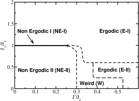
Figure 2: Zero-temperature ergodicity phase diagram in the $J^{\prime}-J_{\perp}$ plane. Due to the symmetry of the Hamiltonian only the upper half is shown (see in the text). Only two ergodic phases (E-I and E-II) have been found in the reported parameter space. The others are either non-ergodic (NE-I and NE-II) or impossible to conclusively analyze (W). The latter phase might shrink to a transition line in the bulk limit.

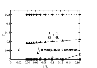
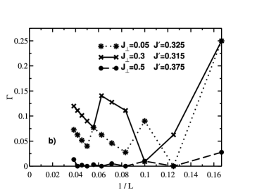
Figure 3: Finite-size scaling in the case of $T=0$ for different points in the phase diagram of Fig. 2. Symbols on panel a): $+$ corresponds to (NE-II), $\blacktriangle$ corresponds to (NE-I), $\blacksquare$ corresponds to (E-I) and $\bigcirc$ to (E-II) regions of Fig. 2, respectively. On panel b) different examples from (W) region are shown. Hamiltonian couplings are shown in the legend. All energies are expressed in units of $J_{z}$.

In the standard Heisenberg model ($J^{\prime}=0$ and $J_{\perp}=J_{z}$) at $T=0$ the dynamics is non-ergodic for ferromagnetic coupling ($J_{\perp}=J_{z}<0$) as the system has a $L+1$ degenerate ground state

$$\Gamma=\frac{1}{12}+\frac{1}{6L}.$$ (2.64)

It is clear from (2.64) that $\Gamma$ remains non-ergodic also in the thermodynamic limit. This point ($J^{\prime}=0$ and $J_{\perp}=J_{z}$) becomes a line in our phase diagram and is denoted as NE-I (see Fig. 2). In fact, the next-nearest-neighbor interaction $J^{\prime}$ may frustrate ($J^{\prime}>0$) or favor ($J^{\prime}<0$) the ferromagnetism. In the latter case, the ground state remains unchanged for any value of $J^{\prime}<0$. Therefore, we expect the line denoting the phase NE-I to extend also to negative $J^{\prime}$. If, on the contrary, $J^{\prime}$ is positive and large enough to frustrate the system in such a way that the ground state loses its ferromagnetic character, the ergodicity is restored. This occurs at a finite critical $J^{\prime}\sim 0.25J_{z}$. For values of $J^{\prime}$ larger than the critical one, we find a non-degenerate ground state with $\langle S^{z}_{tot}\rangle=0$.

If $J_{\perp}\neq J_{z}$ the rotational invariance is broken so that states with the same $\langle{\bf S}_{tot}^{2}\rangle$, but different $\langle S_{tot}^{z}\rangle$, are not degenerate anymore. In the non-ergodic region (NE-II) of the phase diagram (see Fig. 2), the ground state is just doubly degenerate (not $L+1$ degenerate as in (NE-I)): one ground state corresponds to a configuration with all spins up and the other to a configuration with all spins down. Hence, the value of $\Gamma$ in this phase is $1/4$ and does not depend neither on the Hamiltonian couplings nor on the number of sites in the chain. It is clear that also this phase extends to negative values of $J^{\prime}$. This kind of ground state stands the frustration introduced by next-nearest-neighbor interaction up to $J^{\prime}\sim 0.3J_{z}$ (see Fig. 2).

The ergodic region (E-I) of the phase diagram (see Fig. 2) has $\Gamma=0$ for all sizes of the system and values of the couplings: the unique ground state belongs to the sector with $\langle S_{tot}^{z}\rangle=0$. On the contrary, the other ergodic phase (E-II) has non-zero values of $\Gamma$ for values of $L$ not multiples of four. The ground state in this phase has average total spin equal to one and, therefore, $\Gamma=1/L^{2}$. We obviously conclude that (E-II) phase is ergodic in the thermodynamic limit.

The values of $\Gamma$ in these four phases (NE-I, NE-II, E-I and E-II) exhibit perfect finite-size scaling as shown in Fig. 3a). This has allowed us to make definite statements also in the thermodynamic limit.

The weird phase (W) (see Fig. 2) is characterized by a quite strong size dependence, as shown in Fig. 3b) where a tentative finite-size scaling of $\Gamma$ in the different points of the phase is presented. This region manifests a diverging finite-size scaling within the range of sizes we were able to handle. In this case, the behavior of $\Gamma$ as a function of $L$ strongly depends on the particular choice of the Hamiltonian couplings and is highly non monotonous when increasing $L$, according to the strong dependence on $L$ of $\langle S_{tot}^{z}\rangle$ in the ground state. In this critical region the eigenvalues of (2.61) present many level crossings, which means that the maximum value of $L$ we were able to reach ($L_{max}=26$) is not large enough to perform a sensible finite-size scaling analysis. However, we expect that this phase becomes ergodic in the thermodynamic limit, although still different from the ergodic phases E-I and E-II.

We can summarize our findings in the thermodynamic limit at zero temperature as follows:

$$\Gamma=\begin{cases}\frac{1}{12}&\text{if $J_{\perp}=\pm J_{z}$ and $J^{\prime}\lesssim 0.25J_{z}$}\\ \frac{1}{4}&\text{if $|J_{\perp}|<J_{z}$ and $J^{\prime}\lesssim 0.3J_{z}$}\\ ???&\text{in the \emph{weird} phase (W) (see Fig.~{}\ref{fig1})}\\ 0&\text{otherwise}\end{cases}$$ (2.65)

3 Conclusions

In conclusion, we have analyzed the issue of ergodicity, after a brief historical overview, within the Green’s function formalism by means of the equations of motion approach. We have individuated the primary source of non-ergodic dynamics for a generic operator in the appearance of zero-frequency anomaly in its correlation functions and given a recipe to compute the unknown quantities characterizing such a behavior within the Composite Operator Method. Finally, we have presented examples of non-trivial strongly correlated systems where it is possible to examine a non-ergodic behavior: two-site Hubbard model, tight-binding model, Heisenberg chain.

References

- 1. R. Kubo, J. Phys. Soc. Jpn. 12, 570 (1957).
- 2. H. Falk, Phys. Rev. 165, 602 (1968).
- 3. F. Mancini and A. Avella, Condens. Matter Phys. 9, ??? (2006).
- 4. F. Mancini and A. Avella, Adv. Phys. 53, 537 (2004).
- 5. A. I. Khintchin, Mathemathical Foundations of Statistical Mechanics (Dover Publ. Inc., New York, 1949).
- 6. M. Suzuki, Physica 51, 277 (1971).
- 7. T. Morita and S. Katsura, J. Phys. C. 2, 1030 (1969).
- 8. P. C. Kwork and T. D. Schultz, J. Phys. C. 2, 1196 (1969).
- 9. K. W. H. Stevens and G. A. Toombs, Proc. Phys. Soc. 85, 1307 (1965).
- 10. H. Callen, R. H. Swendsen, and R. Tahir-Kheli, Phys. Lett. A 25, 505 (1967).
- 11. J. F. Fernandez and H. A. Gersch, Proc. Phys. Soc. 91, 505 (1967).
- 12. J. G. Ramos and A. A. Gomes, Nuovo Cimento 3A, 441 (1971).
- 13. D. L. Huber, Physica 87A, 199 (1977).
- 14. V. L. Aksenov, H. Konvent, and J. Schreiber, Phys. Stat. Sol. (b) 88, K43 (1978).
- 15. V. L. Aksenov and J. Schreiber, Phys. Lett. A 69, 56 (1978).
- 16. V. L. Aksenov, M. Bobeth, N. M. Plakida, and J. Schreiber, J. Phys. C. 20, 375 (1987).
- 17. A. Avella, F. Mancini, and T. Saikawa, Eur. Phys. J. B 36, 445 (2003).
- 18. M. Bak, A. Avella, and F. Mancini, Phys. Stat. Sol. (b) 236, 396 (2003).
- 19. E. Plekhanoff, A. Avella, and F. Mancini, cond-mat/0606152 (unpublished).