Spin squeezing in optical lattice clocks via lattice-based QND measurements

Abstract

Quantum projection noise will soon limit the best achievable precision of optical atomic clocks based on lattice-confined neutral atoms. Squeezing the collective atomic pseudo-spin via measurement of the clock state populations during Ramsey interrogation suppresses the projection noise. We show here that the lattice laser field can be used to perform ideal quantum non-demolition measurements without clock shifts or decoherence and explore the feasibility of such an approach in theory with the lattice field confined in a ring-resonator. Detection of the motional sideband due to the atomic vibration in the lattice wells can yield signal sizes a hundredfold above the projection noise limit.

I Introduction

Optical atomic clocks based on neutral atoms confined in state independent optical lattices have made dramatic progress recently Takamoto et al. (2005); Ludlow et al. (2006); R. Le Targat et al. (2006). The highest spectral resolution has been achieved in such a system M. M. Boyd et al. (2006), resulting in the clock instability approaching $1\times 10^{-15}$ at 1 s and an overall uncertainty reaching $1\times 10^{-16}$ M. M. Boyd et al. (2007); A. D. Ludlow et al. (2008). The signal to noise ratio (SNR) for $10^{4}$ atoms in these latest experiments is within a factor of two of the quantum projection noise limit A. D. Ludlow et al. (2008). As the lattice clock performance approaches this limit squeezing of the collective atomic pseudo-spin to overcome quantum projection noise Wineland et al. (1992); Santarelli et al. (1999) will lead to dramatic further advances in the clock performance because the number of atoms involved is large. Furthermore, we believe that the precision, control, and isolation from the environment achieved in these metrological lattice systems can be the basis of powerful probes to explore novel quantum dynamics, such as manifested in the collective interactions between an atomic ensemble and an optical cavity Chan et al. (2003); Black et al. (2003); Kruse et al. (2003); Nagorny et al. (2003); Klinner et al. (2006); Brennecke et al. (2007); Horak and Ritsch (2001); Domokos and Ritsch (2003); Mekhov et al. (2007).

An atomic clock can be realized with the Ramsey technique illustrated in Fig. 1(a-c): atoms with two clock states $|g\rangle$ and $|e\rangle$ are driven with two $\pi/2$-pulses separated by a free evolution time $T$. The evolution of the atomic state during this clock sequence (Fig. 1(b)) can be visualized on the Bloch sphere (Fig. 1(c)): The atomic pseudo spin points initially toward the south pole and is rotated around $x$ by the first $\pi/2$-pulse to lie along $y$ at position 1. From there the pseudo spin precesses along the equator to reach position 2 after $T$. This precession is the “ticking” of the atomic clock: The total angle by which the pseudo-spin precesses measures the elapsed time. In order to measure this phase angle the position of the Bloch vector in the equatorial plane has to be translated into a position in the $x$-$z$-plane by the second $\pi/2$-pulse to position 3 where it can be measured through the population difference between the levels which corresponds to the $z$-component of the pseudo-spin.

The projection noise originates in the tip of the collective pseudo-spin not pointing in a sharp direction. Rather the position of the tip of the pseudo-spin is distributed with a width of order $\sqrt{N}$ for $N$ independent atoms. The “hand” of the atomic clock is intrinsically fuzzy. As a consequence two phase angles closer to each other than $1/\sqrt{N}$ cannot be distinguished. This is illustrated in Fig. 2 where we show the sum of the probability distributions of two Bloch vectors that we wish to distinguish. In Fig. 2(a) the two Bloch vectors have accumulated a relative phase of $1/\sqrt{N}$ at the end of the Ramsey pulse sequence at position 3 and hence the two Bloch vectors are not resolved.

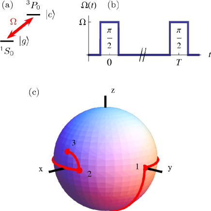
Figure 1: (Color online) (a) $|g\rangle$ and $|e\rangle$ are the two clock states for ⁸⁷Sr. (b) The Ramsey pulse sequence with each pulse having an area of $\pi/2$, and they are separated by a free evolution time $T$ much longer than the duration of each pulse. (c) Illustration of the trajectory of the atomic pseudo spin on the Bloch sphere during the Ramsey pulse sequence. 1: action of the first pulse, 2: free evolution, and 3: action of the second pulse. After the second pulse the population difference of the clock states is measured.

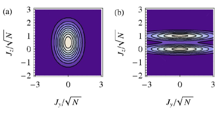
Figure 2: (Color online) Sum of probability distributions at the end of the clock sequence (position 3 in Fig. 1(c)) for two pseudo spin vectors that we wish to resolve in order to distinguish two atom-field detuning values. The pseudo spins have accumulated a relative phase $1/\sqrt{N}$ during the free evolution stage of the Ramsey sequence. In (a) the initial state of the atoms was the conventional state of all atoms in $|g\rangle$ and the two final positions of the pseudo spin cannot be distinguished, giving rise to the shot-noise limit. In (b) on the other hand a spin squeezed state was used and the two positions can be resolved leading to a measurement precision better than the shot-noise limit.

However, the projection noise can be reduced by preparing the atoms in an entangled state in which the distribution of the pseudo spin is squeezed. The principle of this idea is to prepare the atoms in a state such that the distribution of the pseudo spin at the end of the clock sequence is narrower in the $z$-direction, as shown in Fig. 2(b). This way the Bloch vectors of two states that have accumulated less than $1/\sqrt{N}$ of phase difference can be distinguished. The higher phase resolution translates into an increased clock precision. By means of spin squeezing the projection noise can be reduced in principle to the Heisenberg limit which scales with the number of atoms as $1/N$. The Heisenberg limit scaling has been demonstrated in experiments with few entangled ions D. Leibfried et al. (2004); C. F. Roos et al. (2006). For neutral atoms, their large sample number permits a huge reduction of the projection noise Kuzmich et al. (1998); J. Hald et al. (1999).

Spin-squeezed states can be created by means of atom interactions Orzel et al. (2001), interaction with a cavity field Sørensen and Mølmer (2002); Vernac et al. (2000) or through the back-action of quantum non-demolition (QND) measurements J. Hald et al. (1999); Geremia et al. (2004); Chaudhury et al. (2006). Since we are considering the latter approach in this paper we briefly review this type of measurement. For definiteness we discuss the case of measurements of the $z$-component $\hat{J}_{z}$ of the collective atomic pseudo spin. This is no restriction since squeezed states along any direction can be obtained from a state squeezed along the $z$-direction through rotations.

According to the principles of quantum mechanics we are guaranteed to get the same result in a second measurement of any observable as in a first measurement of that observable provided that the observable commutes with the Hamiltonian. This can be considered an extreme case of squeezing: The probability distribution of the observable has collapsed to a delta-function due to the first measurement. This type of measurement is sometimes called a projective measurement. The measurements that are of interest to us in this article are weaker than projective measurements in the sense that several atomic states corresponding to different eigenvalues of the observable are consistent with the measurement outcome. The key point is that, conditioned on the measurement record, some states become more likely than others. This has qualitatively similar consequences for subsequent measurements of the observable as in the projective measurement case. As we keep measuring the observable we are more and more certain about the measurement outcome because only a small range of results will be consistent with the measurement record obtained up to that time. It is essential that these measurements be performed on the same system and not on different copies. Therefore the measurement has to be non-destructive. This type of measurement in which information about the state of the system is extracted gently in such a way that the state of the system persists after the measurement is complete is called a non-demolition measurement. As shown above the resulting state is squeezed.

In our case the observable $\hat{J}_{z}$ is a collective variable. Therefore $\hat{J}_{z}$ cannot be measured through a measurement of each atom’s spin, if we wish to achieve spin squeezing. That would project the atoms on a product state in which each atom’s spin is pointing either up or down. Such a state has a reduced total angular momentum $\langle\hat{J}^{2}\rangle$ and the reduction of the length of the angular momentum outweighs any possible benefits from squeezing. A measurement scheme for spin squeezing must therefore ensure that the total angular momentum $\hat{J}^{2}$ is conserved. Mathematically speaking this means that the Hamiltonian and the interactions describing the measurement must commute with $\hat{J}^{2}$. Physically it means that inhomogeneous broadening has to be negligible during the time scales of interest and the measurement must not be able to distinguish between different particles.

To summarize, a measurement protocol for the preparation of spin-squeezed states should satisfy the following requirements. First, the probe must not lead to decoherence by spontaneous emission or depolarization of the atomic sample by inhomogeneous effects (non-demolition and conservation of $\hat{J}^{2}$ requirements). Second, the measurement must give the population difference with precision exceeding the atomic projection noise. Finally, for clock applications it is important that the measurement does not introduce shifts of the clock transition.

In this article we consider neutral atoms in an optical lattice clock. Conventionally the lattice is treated as an external potential in these systems, i.e. the back-action of the atoms on the light field is neglected. This approximation is motivated by the coupling between atoms and lattice photons being very weak. A large number of photons is necessary to provide a deep enough lattice for the atoms while the many orders of magnitude smaller number of atoms has only a microscopic effect on the light field. However, the minute changes that the lattice fields experience when they propagate through the atomic sample contain information about the atomic state that is normally lost. We show that the information that the atoms imprint on the lattice fields can be harnessed. In particular we propose to use the lattice field itself for the non-demolition measurement of the clock pseudo-spin to achieve spin squeezing. Such a scheme has several advantages over probing the atomic state with an additional interrogation field in addition to using a resource that is normally wasted. Importantly, the lattice does not introduce clock shifts as it operates at the magic frequency where the two clock states have an identical polarizability Takamoto et al. (2005); Ludlow et al. (2006); R. Le Targat et al. (2006); M. M. Boyd et al. (2006, 2007); A. D. Ludlow et al. (2008). Decoherence by spontaneous emission is small since the lattice is far detuned from strong atomic transitions. The lattice laser also couples equally to atoms at different lattice sites due to the lattice periodicity, i.e. the probe is only sensitive to the total pseudo spin and the measurement is of the non-demolition type. According to our list of requirements above it remains to be shown that sufficient precision for spin squeezing can be achieved using this approach. That is the main subject of this article.

In general one has to “level the playing field” between photons and atoms in order for the microscopic effects of the atoms on the light field to become detectable experimentally. Since it is difficult to increase the number of atoms this means that the number of photons has to be reduced. This can be achieved by putting the photons in a cavity. Figuratively speaking each photon passes through the atomic cloud many times and therefore a much smaller number of photons is sufficient to generate the optical lattice. Conversely each photon also accumulates the effect of interaction with the atoms over many round trips so that the signal is enhanced. In this article we consider the case of a bad cavity, in a sense that we will make precise below, for two reasons. First, this is the case that is immediately relevant for the next generation of atomic clocks. Second, we want to use the light field as a measurement device. This implies that the dynamics of the field should be as simple as possible so that the state of the atoms can be read off directly without having to understand the complicated physics of the meter. In a high-Q cavity where the atoms and light field interact with each other in the strong coupling regime their coupled dynamics would be so complicated that it would become hard if not impossible to infer the atomic state from measurements of the field.

The principle of our idea for measuring the atoms’ spin with the lattice fields is the following. The atoms are initially prepared in state $|g\rangle$. During the first Ramsey pulse the clock laser drives them into a 50/50 superposition. If this drive is in the Lamb-Dicke and resolved side-band regime the atoms will remain at rest. The recoil momentum associated with each transition has to be taken up by the lattice fields. If the lattice is generated in a ring cavity this is achieved by transferring photons from one mode to the counter propagating mode. By measuring the intensity redistribution one can determine how much momentum has been exchanged between the two modes or, equivalently, how many transitions have happened. This constitutes a measurement of $\hat{J}_{z}$ since we started from a state with a known $\hat{J}_{z}$ quantum number.

The rest of this article is organized as follows. In section II we introduce the model and develop the theoretical framework that we will use. Section III discusses the measurement scheme outlined in the previous paragraph. As we will see, the signal to noise ratio (SNR) of this measurement is insufficient to achieve spin squeezing for currently realizable lattice clocks. Section IV is dedicated to a superior measurement scheme based on detecting motional sidebands of the atoms that promises to lead to a strong enough signal that can yield significant spin squeezing. We draw conclusions in section V.

II Model

We consider $N$ two-level atoms with ground state $|g\rangle$, excited state $|e\rangle$, and transition frequency $\omega_{a}$, trapped in a one-dimensional optical lattice generated by the two counter propagating running wave modes of a ring cavity with frequency $\omega_{L}$ (Fig. 3). The projections of the running waves’ wave vectors along the $z$-axis are $k_{L}=\cos\theta\;\omega_{L}/c$ and $-k_{L}$, where $\theta$ is the angle at which clock laser and the lattice beams cross. The transverse profile of the modes is approximately Gaussian and we neglect the dependence of its radius $w_{0}$ on $z$. The cavity length is $L$. The atomic transition is probed by a highly stabilized clock laser of frequency $\omega_{c}$, which is linearly polarized in the same direction as the lattice.

II.1 Effective Hamiltonian

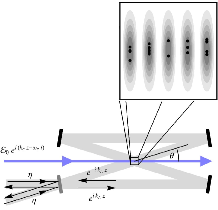
Figure 3: (Color online) Schematic of the lattice in the ring resonator with atoms trapped at the intensity anti-nodes. The clock laser propagates along the $z$ axis and the projection of the wave numbers of the counter propagating lattice modes along the $z$-axis is $k_{L}$ and $-k_{L}$. The lattice light leaking out of the resonator contains information about the atomic state. The clock laser wave vector is commensurate with the reciprocal lattice period under this particular lattice geometry. Details of coupling into and out of the ring cavity as well as the detector arrangement are given in Fig. 4.

In our calculations, we neglect inhomogeneous effects. This is justified if the duration of the clock pulse sequence is smaller than the $T_{2}$ time associated with the inhomogeneities. The main source of inhomogeneous broadening in experiments is due to the radial distribution of atoms in the 1D optical lattice which is typically only weakly confining in the transverse direction. The inhomogeneities stemming from this can be eliminated by confining the atoms in a 3D lattice. We assume that the wavefunction of the atoms can be factorized into a part for spin and $z$ on the one hand and all other degrees of freedom on the other hand. Since we will be only interested in spin and $z$, considering just that part of the wavefunction is sufficient, leading to an effectively 1D theory. The initial state, all atoms in $|g\rangle$ and vibrational ground state ,

$$|\psi(t=0)\rangle=\underbrace{|g,n=0;\;g,n=0;\ldots;\;g,n=0\rangle}_{N\;\rm times},$$ (1)

is completely symmetric under particle exchange with respect to the pseudo-spin and $z$ which are the degrees of freedom relevant to us. The system will remain in the totally symmetric subspace since inhomogeneities are negligible. Hence we can use a totally symmetrized basis and going over to the usual second quantized formalism we can effectively treat the atoms as bosons.

The system can be described with the Hamiltonian

$$\hat{H} = \frac{-\hbar^{2}}{2M}\sum_{\sigma=g,e}\int dz\;\hat{\psi}_{\sigma}^{\dagger}(z)\frac{\partial^{2}}{\partial_{z}^{2}}\hat{\psi}_{\sigma}(z)+\hbar g_{0}\sum_{\sigma=g,e}\int dz\;(e^{-ik_{L}z}\hat{a}_{k_{L}}^{\dagger}+e^{ik_{L}z}\hat{a}_{-k_{L}}^{\dagger})(e^{ik_{L}z}\hat{a}_{k_{L}}+e^{-ik_{L}z}\hat{a}_{-k_{L}})\hat{\psi}_{\sigma}^{\dagger}(z)\hat{\psi}_{\sigma}(z)$$ (2)

$$+\frac{\hbar\Omega}{2}\left(e^{-i\delta t}\int dz\;e^{ik_{c}z}\hat{\psi}_{e}^{\dagger}(z)\hat{\psi}_{g}(z)+H.C.\right)+\sum_{p=\pm k_{L}}\left(-\hbar\Delta\hat{a}_{p}^{\dagger}\hat{a}_{p}+\hbar\eta(\hat{a}_{p}^{\dagger}+\hat{a}_{p})\right).$$

$\hat{\psi}_{e}$ and $\hat{\psi}_{g}$ are bosonic field operators describing the atoms in the excited and ground states. The first term in the Hamiltonian is the atomic kinetic energy, with $M$ being the atomic mass. The second term describes the lattice potential. $g_{0}=\frac{\alpha\omega_{L}}{\pi\epsilon_{0}w_{0}^{2}L}$ is the coupling constant between atoms and the lattice field. $\alpha$ is the common polarizability of $|g\rangle$ and $|e\rangle$. $\hat{a}_{\pm k_{L}}$ are bosonic field operators for the running wave modes of the ring resonator. The third term describes the drive of the atomic transition by the clock laser with a Rabi frequency $\Omega$ and detuning $\delta=\omega_{c}-\omega_{a}$. The last term represents the detuning $\Delta$ of the lattice laser from the resonator mode and the pump of the lattice field with amplitude $\eta$, which is assumed to be real. The losses of both modes with decay constant $\kappa$ can be described by means of a standard Born-Markov Liouville operator

$$\hat{L}[\hat{\rho}]=-\frac{\hbar\kappa}{2}\sum_{p=\pm k_{L}}(\hat{a}_{p}^{\dagger}\hat{a}_{p}\hat{\rho}+\hat{\rho}\hat{a}_{p}^{\dagger}\hat{a}_{p}-2\hat{a}_{p}\hat{\rho}\hat{a}_{p}^{\dagger}),$$ (3)

where $\hat{\rho}$ is the system density operator. We neglect spontaneous emission from $|e\rangle$ which is justified because the lifetime of that level is many times longer than the clock sequence considered here.

The periodic arrangement of atoms in the lattice strongly couples the two counter propagating modes with a coupling frequency of order $g_{0}N$. The symmetric cosine and antisymmetric sine modes described by the field operators

$$\hat{b}_{\pm}=\frac{1}{\sqrt{2}}\left(\hat{a}_{k_{L}}\pm\hat{a}_{-k_{L}}\right)$$ (4)

on the other hand are uncoupled for a perfect atomic lattice and weakly coupled if the density distribution is slightly perturbed. Since it is exactly these small deviations of the atomic density distribution from the perfect lattice caused by the clock laser that we wish to detect, we transform the lattice field to the symmetric and antisymmetric modes $\hat{b}_{+}$ and $\hat{b}_{-}$. Because the cavity pumping amplitude $\eta$ is real only the symmetric mode is pumped. In steady state the symmetric mode $\hat{b}_{+}$ has therefore a large mean amplitude $\beta_{+}$ which gives rise to the lattice. The steady state amplitude can be found from the equations of motion

$$i\frac{d\langle\hat{b}_{+}\rangle}{dt} = -(\Delta+i\frac{\kappa}{2})\langle\hat{b}_{+}\rangle+g_{0}\int dz\sum_{\sigma}\langle\hat{\psi}_{\sigma}^{\dagger}(z)\hat{\psi}_{\sigma}(z)\rangle\times$$ (5)

$$\left(2\cos^{2}k_{L}z\;\langle\hat{b}_{+}\rangle+i\sin 2k_{L}z\;\langle\hat{b}_{-}\rangle\right)+\sqrt{2}\eta,$$

where we have used that the expectation values like $\langle\hat{b}_{+}\hat{\psi}_{\sigma}^{\dagger}\hat{\psi}_{\sigma}\rangle$ etc. factorize in steady state to a good approximation. We find $\beta_{+}$ by setting $d\langle\hat{b}_{+}\rangle/dt=0$,

$$\beta_{+}=\frac{\sqrt{2}\eta}{\Delta+i\frac{\kappa}{2}-2g_{0}\mathcal{C}(0)},$$ (6)

where we have used $\langle\hat{b}_{-}\rangle=0$ in steady state and we have introduced

$$\mathcal{C}(t)=\int dz\sum_{\sigma}\cos^{2}k_{L}z\langle\psi_{\sigma}^{\dagger}(z)\psi_{\sigma}(z)\rangle.$$ (7)

We eliminate $\beta_{+}$ with the canonical transformation $\hat{b}_{+}\rightarrow\hat{d}_{+}+\beta_{+},\;\hat{b}_{-}\rightarrow\hat{d}_{-}$. $\beta_{+}$ gives rise to an optical lattice of depth $2\hbar|\beta_{+}|^{2}g_{0}$. Assuming a deep lattice, we can neglect tunneling between different lattice sites and approximate the lattice with a harmonic potential at each site.

The atom-lattice coupling is trivially lattice periodic. The clock-laser-atom interaction can also be made lattice periodic by crossing the lattice modes at an angle such that $k_{c}=2k_{L}$. Atoms on different sites are then indistinguishable and by transforming the coordinates of a particle trapped on site $j$ according to $z\rightarrow z-j\pi/k_{L}$ we can treat them as if they were all trapped in a single harmonic well. This interpretation makes precise what is meant by the initial state Eq. (1). The indistinguishability of atoms at different sites is also important from a practical point of view because it allows one to squeeze the pseudo-spin for all atoms, not just the atoms at each lattice site.

We expand the atomic field operators in an energy basis $\varphi_{n}(z)$ of the single harmonic oscillator representing the lattice,

$$\hat{\psi}_{\sigma}(z)=\sum_{n}\varphi_{n}(z)\hat{c}_{\sigma,n},$$ (8)

with oscillator frequency $\omega_{\rm osc}=\sqrt{4\hbar|g_{0}||\beta_{+}|^{2}k_{L}^{2}/M}$ and oscillator length $a_{\rm osc}=\sqrt{\hbar/(M\omega_{\rm osc})}$. We assume that the atoms are deep in the Lamb-Dicke regime which for atoms in the first few vibrational states means $k_{L}a_{\rm osc},\;k_{c}a_{\rm osc}\ll 1.$

II.2 Mean field equations

In the rest of this article, we study this system in the mean field approximation. The mean field equations of motion for the field amplitudes $\langle\hat{d}_{\pm}\rangle$ and the atomic amplitudes $\langle\hat{c}_{\sigma,n}\rangle$ are found from the Liouville equation for the density matrix

$$\frac{d\hat{\rho}(t)}{dt}=\frac{-i}{\hbar}[\hat{H},\,\hat{\rho}]+\mathcal{L}[\hat{\rho}].$$ (9)

These equations close if we factorize the correlations between atoms and light field according to $\langle\hat{d}_{\pm}\hat{c}_{\sigma,n}\rangle\rightarrow\langle\hat{d}_{\pm}\rangle\langle\hat{c}_{\sigma,n}\rangle$, $\langle\hat{d}_{\pm}^{\dagger}\hat{d}_{\pm}\rangle\rightarrow\langle\hat{d}_{\pm}^{\dagger}\rangle\langle\hat{d}_{\pm}\rangle$, etc. We find

$$i\frac{d\langle\hat{c}_{e,n}\rangle}{dt} = n\omega_{\rm osc}\langle\hat{c}_{e,n}\rangle+\frac{\Omega e^{-i\delta t}}{2}\sum_{n^{\prime}}\langle n|e^{ik_{c}z}|n^{\prime}\rangle\langle\hat{c}_{g,n^{\prime}}\rangle$$

$$+i\hbar g_{0}\left((\beta^{*}_{+}+\langle\hat{d}_{+}^{\dagger}\rangle)\langle\hat{d}_{-}\rangle-(\beta_{+}+\langle\hat{d}_{+}\rangle)\langle\hat{d}_{-}^{\dagger}\rangle\right)\sum_{n^{\prime}}\langle n|\sin\,2k_{L}z|n^{\prime}\rangle\langle\hat{c}_{e,n^{\prime}}\rangle,$$

$$i\frac{d\langle\hat{c}_{g,n}\rangle}{dt} = n\omega_{\rm osc}\langle\hat{c}_{g,n}\rangle+\frac{\Omega e^{i\delta t}}{2}\sum_{n^{\prime}}\langle n|e^{-ik_{c}z}|n^{\prime}\rangle\langle\hat{c}_{e,n^{\prime}}\rangle$$

$$+i\hbar g_{0}\left((\beta^{*}_{+}+\langle\hat{d}_{+}^{\dagger}\rangle)\langle\hat{d}_{-}\rangle-(\beta_{+}+\langle\hat{d}_{+}\rangle)\langle\hat{d}_{-}^{\dagger}\rangle\right)\sum_{n^{\prime}}\langle n|\sin\,2k_{L}z|n^{\prime}\rangle\langle\hat{c}_{g,n^{\prime}}\rangle,$$

$$i\frac{d\langle\hat{d}_{-}\rangle}{dt} = -(\Delta-2g_{0}\mathcal{S}(t)+i\kappa/2)\langle\hat{d}_{-}\rangle-ig_{0}(\beta_{+}+\langle\hat{d}_{+}\rangle)\mathcal{S}_{2}(t),$$ (12)

$$i\frac{d\langle\hat{d}_{+}\rangle}{dt} = -(\Delta-2g_{0}\mathcal{C}(t)+i\kappa/2)\langle\hat{d}_{-}\rangle+ig_{0}\langle\hat{d}_{-}\rangle\mathcal{S}_{2}(t)+g_{0}(\mathcal{C}_{2}(t)-\mathcal{C}_{2}(0))\beta_{+}.$$ (13)

We have introduced

$$\mathcal{S}(t) = \sum_{\sigma}\int dz\;\sin^{2}\,k_{L}z\langle\hat{\psi}_{\sigma}^{\dagger}(z)\hat{\psi}_{\sigma}(z)\rangle,$$ (14)

$$\mathcal{S}_{2}(t) = \sum_{\sigma}\int dz\;\sin\,2k_{L}z\langle\hat{\psi}_{\sigma}^{\dagger}(z)\hat{\psi}_{\sigma}(z)\rangle,$$ (15)

and

$$\mathcal{C}_{2}(t)=\sum_{\sigma}\int dz\;\cos\,2k_{L}z\langle\hat{\psi}_{\sigma}^{\dagger}(z)\hat{\psi}_{\sigma}(z)\rangle.$$ (16)

II.3 Approximations

In the Lamb-Dicke and resolved sideband regime the density distribution of the atoms does not change much during the evolution. In particular we have

$$\mathcal{C}_{2}(t)-\mathcal{C}_{2}(0)=\mathcal{O}((k_{L}a_{\rm osc}\frac{\Omega}{\omega_{\rm osc}})^{2}).$$ (17)

Neglecting this small term in Eq. (13) is an excellent approximation for the cases we are interested in.

With this approximation it is clear that the modes $\hat{d}_{-}$ and $\hat{d}_{+}$ are no longer pumped. Light is scattered into these modes exclusively through interaction with the atoms and we find the scalings

$$\langle\hat{d}_{+}\rangle\sim\frac{g_{0}\mathcal{S}_{2}(t)}{\kappa}\langle\hat{d}_{-}\rangle,\quad\langle\hat{d}_{-}\rangle\sim\frac{g_{0}\mathcal{S}_{2}(t)}{\kappa}\beta_{+}.$$ (18)

As discussed in the introduction we consider the bad cavity limit. The previous equation motivates the appropriate condition for the bad cavity limit,

$$\frac{g_{0}\mathcal{S}_{2}(t)}{\kappa}\ll 1.$$ (19)

The resulting hierarchy of the amplitudes $\langle\hat{d}_{+}\rangle\ll\langle\hat{d}_{-}\rangle\ll\beta_{+}$ allows us to make further approximations: We neglect the symmetric mode altogether, $\langle\hat{d}_{+}\rangle\equiv 0$, and we neglect the back-action of the field on the atoms in Eqs. (II.2,II.2) which is of order $g_{0}\beta_{+}\langle\hat{d}_{-}\rangle$ compared to the lattice potential of order $g_{0}\beta_{+}^{2}$ contained in $\omega_{\rm osc}$.

We end up with a theory in which the atoms move in the steady state lattice potential and are driven by the clock laser. Through $\mathcal{S}_{2}(t)$ they are a source for the $\langle\hat{d}_{-}\rangle$ field.

III Intensity imbalance

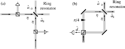
Figure 4: In- and out-coupling into the ring cavity as well as detector arrangements for the two measurement schemes discussed in the text. In (a) two phase-locked lasers pump the two counter propagating modes of the ring cavity and the light leaking out of each mode is picked up with beam splitters. In (b) an incoming pump beam is sent through a Mach-Zehnder interferometer-like arrangement with a $\pi/4$ phase shift in one of the arms. This way the symmetric superposition $\hat{b}_{+}$ of the two running wave modes is pumped. The $\hat{d}_{-}$ amplitude leaks out of the empty port of the Mach-Zehnder interferometer where its intensity is measured.

As discussed in the introduction our goal is to find the population difference between electronic excited and ground states after a $\pi/2$-pulse by measuring the momentum transfer between the $+k_{L}$ and $-k_{L}$ modes. A schematic of the detector arrangement for this measurement is shown in Fig. 4(a).

To find the intensity imbalance between the modes we integrate the mean field equations of motion numerically. From the numerical solutions for the amplitudes inside the cavity we find the intensity difference at the cavity output

$$\delta I=\kappa\langle\hat{a}_{k_{L}}^{\dagger}\hat{a}_{k_{L}}-\hat{a}_{-k_{L}}^{\dagger}\hat{a}_{-k_{L}}\rangle=2\kappa{\rm Re}\;\beta_{+}^{*}\langle\hat{d}_{-}\rangle.$$ (20)

Of course there will be noise in the measurement of the intensity imbalance. In order to find out whether this QND scheme is suitable for spin squeezing we have to determine whether it is possible to measure the number difference with a precision better than the atomic shot noise despite the noise in the intensity imbalance.

We assume that the detection of the intensities of the two modes is (photon-) shot noise limited. The photon shot noise in each port is $\sqrt{\langle\hat{a}_{\pm k_{L}}^{\dagger}\hat{a}_{\pm k_{L}}\rangle}$ . The resulting SNR can be calculated as

$$\text{SNR}_{1}=\frac{\int_{0}^{\frac{\pi}{2\Omega}}dt\kappa\langle\hat{a}_{k_{L}}^{\dagger}\hat{a}_{k_{L}}-\hat{a}_{-k_{L}}^{\dagger}\hat{a}_{-k_{L}}\rangle}{\sqrt{\int_{0}^{\frac{\pi}{2\Omega}}dt\kappa\langle\hat{a}_{k_{L}}^{\dagger}\hat{a}_{k_{L}}+\hat{a}_{-k_{L}}^{\dagger}\hat{a}_{-k_{L}}\rangle}}.$$ (21)

Figure 5 shows the result as a function of the drive strength $\Omega$ of the clock transition for realistic lattice clock parameters. The clock laser is resonant with the $n=0\rightarrow n=0$ transition, i.e. $\delta=0$. The lattice laser amplitude $\eta$ has been adjusted to give $\omega_{\rm osc}=20\omega_{\rm rec}$, where $\omega_{\rm rec}=\hbar\omega_{L}^{2}/(2Mc^{2})$ is the recoil frequency at the lattice wavelength. We have assumed that the atoms are driven from ground to excited state with a $\pi/2$-pulse as they would during the first pulse of a Ramsey sequence. The detector outputs are recorded only during the pulse as indicated by formula Eq. (21).

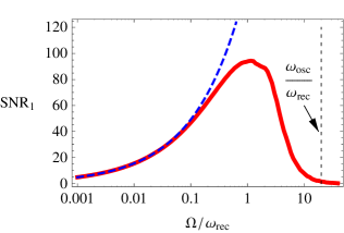
Figure 5: (Color online) SNR for detection of the intensity imbalance during a $\pi/2$-pulse for $10^{6}$ ⁸⁷Sr atoms in a ring cavity of length $L$ = 1 cm, finesse $F=10^{6}$, and waist $w_{0}$ = 30 $\mu$m. $\omega_{\rm osc}=20\omega_{\rm rec}$ and $\delta=0$ (red solid line). The lattice laser is tuned to the magic wavelength $\lambda_{L}=813nm$ and the polarizability at that wavelength is $\alpha=-5.37\times 10^{-28}\text{m}^{3}\epsilon_{0}$. The blue dashed line indicates the analytic result (Eq. (22)) in the adiabatic limit.

In the resolved side band limit $\Omega\ll\omega_{\rm osc}$ we can obtain an approximate analytical solution of the mean field equations of motion by assuming that the coherences between different harmonic oscillator levels follow the drive adiabatically. From the adiabatic solutions for the atomic amplitudes we can then in turn find adiabatic solutions for the light field provided that the strength of the clock laser coupling is well within the band-width of the cavity, $\Omega\ll\kappa$. Once we have the amplitudes of the lattice modes we can calculate the signal to noise ratio using Eq. (21). We find

$${\rm SNR}_{1}^{\rm ad.}=\frac{Nk_{c}/k_{L}}{\sqrt{\frac{\pi\kappa\omega_{\rm osc}^{2}}{16|g_{0}|\Omega\omega_{\rm rec}}}}.$$ (22)

As can be seen in Fig. 5, the analytical solution agrees very well with the numerical results in the limit $\Omega/\omega_{\rm osc}\ll 1$.

The SNR falls off for small $\Omega$ because the signal strength is limited by a photon redistribution of order $\sim N/2$ while the number of photons that contribute to the shot noise keeps increasing over longer intervals $\pi(2\Omega)^{-1}$. At large $\Omega$ the SNR falls off because more and more momentum is taken up by the atoms as they are driven harder and accordingly less intensity needs to be redistributed between the lattice modes to ensure conservation of total momentum. The maximum SNR is obtained near $\Omega\approx\omega_{\rm osc}$ . Assuming that the expression Eq. (22) still holds, we estimate the maximum SNR as

$${\rm SNR}^{\rm max}_{1}=\sqrt{N}\frac{4}{\sqrt{\pi}}\frac{k_{c}}{k_{L}}\sqrt{\frac{\omega_{\rm rec}}{\omega_{\rm osc}}}\sqrt{\frac{Ng_{0}}{\kappa}}.$$ (23)

This simple scaling law is one of the key results of this paper. In order for the measurement to lead to spin squeezing, the $\rm{SNR}$ has to be sufficiently large such that the measurement uncertainty is smaller than the atomic projection noise, i.e., ${\rm SNR}>N/\Delta N\sim\sqrt{N}$. In other words the measurement has to be atomic shot noise limited. Since $4k_{c}(\sqrt{\pi}k_{L})^{-1}(\omega_{\rm rec}/\omega_{\rm osc})^{1/2}$ is typically of order one and is hard to vary in experiments the collective coupling parameter $Ng_{0}\kappa^{-1}$ is the all important parameter. Note that we can be in the strong collective coupling regime Klinner et al. (2006) $Ng_{0}\kappa^{-1}\gg 1$ while still in the bad cavity limit in the sense of Eq. (19) because $\mathcal{S}_{2}(t)\ll N$ in the Lamb-Dicke and resolved side band regime.

It can be seen from Eq. (23) and Fig. 5 that a $\rm{SNR}$ greater than $\sqrt{N}$ is hard to achieve with currently realistic lattice clocks but it might not be completely out of reach in the future. The collective coupling parameter is small in these systems primarily because of the requirement of operating the lattice at the magic wavelength. The magic wavelength is typically very far removed from atomic resonances. Therefore the atomic polarizability is very small, giving rise to a small single atom coupling constant $g_{0}$. The fundamental reason for the rather limited $\rm{SNR}$ is the intrinsic photon shot noise of the lattice beams, i.e. the measurement is photon-shot noise limited rather than atom-shot noise limited. The momentum transfer from the clock laser to the lattice laser that has to be measured is smaller than the large momentum uncertainties stemming from the photon shot noise in the lattice beams. In the conclusion section we discuss methods that may improve the SNR of this scheme to a level where it becomes a viable means to obtain spin squeezing. However, we will first introduce a much more promising approach in the next section for measurement-induced spin squeezing.

IV Sideband spectroscopy

In this section we describe a superior detection method that is not affected by the large photon shot noise in the lattice beams that dominated the SNR in the detection method discussed in the previous section. The general idea is to design a measurement in which the signal can be separated from the lattice beams. The motional sidebands generated by the atoms oscillating in the lattice with frequencies $\pm\omega_{\rm osc}$ are such a signal. In a heterodyne detector with bandwidth much smaller than $\omega_{\rm osc}$ the sidebands can be distinguished from the carrier at $\omega_{L}$, provided that the line width of the lattice is smaller than $\omega_{\rm osc}$ which is achieved experimentally.

In order for the detection of atomic vibration to constitute a measurement of the populations of atomic electronic states these two quantities must be strongly correlated. If for instance only atoms of one electronic state are oscillating while the other is at rest, detection of the sideband can measure the number of atoms in the oscillating state. Other possibilities would be to have atoms of both states oscillate with the same amplitude but $\pi/2$ or $\pi$ out of phase. If the atoms oscillate $\pi/2$ out of phase the populations of the two states are proportional to the intensities in the two quadratures of the sidebands. If they oscillate $\pi$ out of phase, the intensity of the sidebands is directly proportional to the number difference of the two states.

Such correlated states of atomic motion and internal level are created rather naturally in lattice clocks. To see this we consider the atomic dynamics during a $\pi/2$-pulse starting from initial state Eq. (1). The limit of a strong pulse $\Omega\gg\omega_{\rm osc}$ is easy to understand intuitively. In this case the component of the atoms that undergoes a transition to the excited state receives $N_{e}\hbar k_{c}$ of recoil momentum where $N_{e}$ is the final population of the excited state, while the atoms that stay in the ground state remain at rest. After the $\pi/2$-pulse only the excited state component will oscillate at frequency $\omega_{\rm osc}$.

The atomic motion is more complex in the weak drive limit $\Omega\ll\omega_{\rm osc}$. Because atoms exchange momentum with the lattice lasers while absorbing and reemitting clock photons it is clear that both states start oscillating. The atoms’ dynamics is illustrated in Fig. 6. During the pulse the atoms in the two electronic states oscillate $\pi$ out of phase with each other but with equal envelope. The amplitude of the oscillations is suppressed compared to the strong pulse limit by a factor $k_{c}a_{\rm osc}\Omega/\omega_{\rm osc}$. If the pulse duration is $t_{\pi/2}\omega_{\rm osc}=m2\pi$ with $m$ an integer, only the ground state oscillates after the pulse. For $t_{\pi/2}\omega_{\rm osc}=(m+1/2)2\pi$ only the excited state oscillates and for $t_{\pi/2}\omega_{\rm osc}=(m\pm 1/4)\pi$ both states oscillate with equal amplitude. The oscillations after the pulse are undamped to a good approximation for $\kappa\gg\omega_{\rm osc}$ and $\Delta=2g_{0}N$ regardless of the strength of $\Omega$ Domokos and Ritsch (2003); Horak and Ritsch (2001).

For the numerical examples in this section we consider a cavity with reduced finesse $F=10^{4}$ (corresponding to $\kappa\approx 2\pi\;(3\;{\rm MHz})$ for $L=1$ cm) compared to the example in the previous section to ensure that $\kappa\gg\omega_{\rm osc}$. All other parameters are as before.

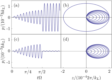
Figure 6: (Color online) Momentum per atom in ground (a) and excited state (c) during a $\pi/2$-pulse with $\Omega=0.5\omega_{\rm rec}$. Figures (b) and (d) show the corresponding phase space trajectories for atoms in ground and excited state, respectively. At the beginning of the pulse the atoms are at rest at the origin, $p=0$ and $z=0$. During the pulse the atoms oscillate on ellipses of growing diameter. When the pulse terminates at $t=\pi/2/\Omega$ the atoms in the ground state are at the turning point on the right. Therefore they continue to oscillate with large amplitude in the harmonic trap after the pulse. The excited state on the other hand is at the origin at the end of the pulse. It therefore remains essentially at rest after the pulse.

We now turn to a quantitative discussion of the measurement of the atomic vibration using the lattice fields. As before we assume that we are in the bad cavity limit Eq. (19) and we retain $\langle\hat{d}_{-}\rangle$ and neglect $\langle\hat{d}_{+}\rangle$. We consider the situation outlined above where $t_{\pi/2}\omega_{\rm osc}=m2\pi$ such that the excited state is at rest after the $\pi/2$ pulse. The amplitude $\langle\hat{d}_{-}\rangle$ is then fed by a source

$$g_{0}\sum_{n,n^{\prime},\sigma}\langle n|\sin\,2k_{L}z|n^{\prime}\rangle\langle\hat{c}_{n,\sigma}^{\dagger}\rangle\langle\hat{c}_{n^{\prime},\sigma}\rangle\approx g_{0}N_{g}\bar{z}_{g}\sin(\omega_{\rm osc}t-\phi_{g}),$$ (24)

where $N_{g}$ is the population of the ground state and $\bar{z}_{g}$ and $\phi_{g}$ are the amplitude and phase of the oscillations of the ground state atoms.

In order to evaluate the suitability of this scheme for spin squeezing we need to calculate the SNR for measuring the intensity of the sideband $\langle\hat{d}_{-}\rangle$ . For heterodyne detection with a strong local oscillator the SNR is

$${\rm SNR_{2}}=\int_{t_{\pi/2}}^{t_{\pi/2}+T}dt\kappa|\langle\hat{d}_{-}\rangle|^{2},$$ (25)

where $T$ is the integration time and we start the measurement immediately after the $\pi/2$-pulse. With a strong local oscillator every $\hat{d}_{-}$ photon is detected and the SNR is equal to the total number of photons scattered from the symmetric mode into the $\hat{d}_{-}$ mode. The SNR can be readily evaluated using the numerical solutions for the field amplitude. The result is shown in Fig. 7 for an integration time of 1 s as a function of $\Omega$. As in the previous section the weak drive limit can be studied analytically by assuming that the coherences between the different atomic vibrational levels follow the drive adiabatically. The adiabatic result,

$${\rm SNR}_{2}^{\rm ad.}=\frac{(k_{c}/k_{L})^{2}N^{2}\Omega^{2}\kappa T}{32(\Delta^{2}+(\kappa/2)^{2})|\beta_{+}|^{2}},$$ (26)

is also shown in Fig. 7 and agrees well with the numerical result. The amplitude of the atoms’ oscillations decreases as the strength of the drive is reduced according to the aforementioned suppression by $\Omega/\omega_{\rm osc}$, resulting in a weaker generated signal and accordingly a smaller SNR.

In the strong drive limit the atoms eventually take up all the recoil momentum $(N/2)\hbar k_{c}$ and the SNR saturates at

$${\rm SNR}_{2}^{\rm max}=\frac{(k_{c}k_{L}a_{\rm osc}^{2})^{2}N^{2}|\beta_{+}|^{2}g_{0}^{2}\kappa T}{2(\Delta^{2}+(\kappa/2)^{2})}.$$ (27)

Figure 7 shows that for $\Omega$ $\sim$ $\omega_{\rm rec}$, a SNR $>$$10^{5}$ can be achieved. For $10^{6}$ atoms, this corresponds to a measurement uncertainty a hundredfold smaller than the projection noise, indicating that spin squeezing becomes possible with this measurement scheme. Note that even at $\Omega\sim\omega_{\rm rec}$, the population of the first excited vibrational state is suppressed by a factor of $(k_{c}a_{\rm osc}(\Omega/\omega_{\rm osc}))^{2}\approx 10^{-4}$ relative to the vibrational ground state, thus maintaining the validity of the Lamb-Dicke regime.

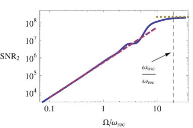
Figure 7: (Color online) SNR for 1 s of detection at the vibrational sideband for ⁸⁷Sr. The asymptotic solutions for weak and strong drives, Eqs. (26) and (27), are shown as the dashed and dotted lines, respectively. Parameters are as in Fig. 5 except that the cavity finesse is $F=10^{4}$.

V Conclusion

We have studied the feasibility of measuring the populations of clock states using the lattice field of an optical lattice clock, with the goal of squeezing the atomic pseudo-spin. We have demonstrated that a measurement of population transfer based on detection of momentum redistribution between the lattice beams is possible but, with current experimental technology, not sensitive enough to enable spin squeezing.

The reason for this failure is that the collective atom lattice coupling $Ng_{0}/\kappa$ is too small for a lattice operating at the magic wavelength. A possible solution might be to operate the lattice at other magic frequencies where $g_{0}$ is larger. Engineering the magic wavelength with external electric, magnetic or laser fields such that it is closer to an atomic resonance might be another option. Stronger coupling can also be achieved with a smaller volume cavity.

A second measurement scheme based on detecting the motional sidebands of atoms after a clock pulse is promising. The SNR that we calculated for realistic parameters appropriate for a ${}^{87}{\rm Sr}$ lattice clock suggests that spin squeezing could be feasible with this method.

Several questions will have to be addressed in the future. First it will be important to go beyond the harmonic approximation in which the optical lattice is treated as a single harmonic trap. Among other things this will allow us to elucidate the role of tunneling and the band structure during and after the clock pulses. Second the system needs to be studied in the good cavity limit. The good cavity limit is particularly interesting since our results indicate that the two detection schemes presented here work better in cavities with higher $Q$-factor.

Already in the bad cavity, but especially in the good cavity case, it will be necessary to go beyond the mean field approximation. That would allow one to study in detail how the noise in one of the pseudo spin components is reduced at the expense of the other components. Such a beyond meanfield treatment is indispensable for finding the ultimate resolution limits of the spin measurements presented here. Possible routes are cumulant expansion of the atomic and lattice field operators, Langevin equations and Monte-Carlo wavefunction methods.

A question of fundamental interest arising in the context of the second measurement scheme is that in that case we are trying to measure states that are neither eigenstates of the Hamiltonian nor of the operator $\sin 2k_{L}z$ with which the light field couples to the atoms. Instead we are trying to differentiate between states that differ in their dynamics, i.e. one of them is oscillating while the other is at rest. A measurement can therefore not be done instantaneously since this would project the system on eigenstates of $\sin 2k_{L}z$. Rather one has to carefully erase all information about the time at which a photon has been scattered from the symmetric mode into the antisymmetric mode by having the photons circulate in the cavity for a sufficiently long time before they leak out.

We also plan to investigate the prospects of quantum feedback control Geremia et al. (2004); Thomsen et al. (2002) that should allow one to not only prepare the many-particle state probabilistically in squeezed states with a certain $J_{z}$ projection, but also to deterministically drive the system to a target $J_{z}$ projection.

We acknowledge fruitful discussions with H. J. Kimble, P. Jessen, M. M. Boyd, A. Ludlow, and H. Ritsch. This work has been supported by DOE, NIST, and NSF. D. M. gratefully acknowledges support from DAAD. His email address is dmeiser@jila.colorado.edu.

References

- Takamoto et al. (2005) M. Takamoto, F.-L. Hong, R. Higashi, and H. Katori, Nature (London) 435, 321 (2005).
- Ludlow et al. (2006) A. D. Ludlow, M. M. Boyd, T. Zelevinsky, S. M. Foreman, S. Blatt, M. Notcutt, T. Ido, and J. Ye, Phys. Rev. Lett. 96, 033003 (pages 4) (2006).
- R. Le Targat et al. (2006) R. Le Targat et al. , Phys. Rev. Lett. 97, 130801 (2006).
- M. M. Boyd et al. (2006) M. M. Boyd et al., Science 314, 1430 (2006).
- M. M. Boyd et al. (2007) M. M. Boyd et al., Phys. Rev. Lett. 98, 083002 (2007).
- A. D. Ludlow et al. (2008) A. D. Ludlow et al., Science 319, 1805 (2008).
- Wineland et al. (1992) D. J. Wineland, J. J. Bollinger, W. M. Itano, F. L. Moore, and D. J. Heinzen, Phys. Rev. A 46, R6797 (1992).
- Santarelli et al. (1999) G. Santarelli, P. Laurent, P. Lemonde, A. Clairon, A. G. Mann, S. Chang, A. N. Luiten, and C. Salomon, Phys. Rev. Lett. 82, 4619 (1999).
- Klinner et al. (2006) J. Klinner, M. Lindholdt, B. Nagorny, and A. Hemmerich, Phys. Rev. Lett. 96, 023002 (2006).
- Chan et al. (2003) H. W. Chan, A. T. Black, and V. Vuletić, Phys. Rev. Lett. 90, 063003 (2003).
- Black et al. (2003) A. T. Black, H. W. Chan, and V. Vuletić, Phys. Rev. Lett. 91, 203001 (2003).
- Kruse et al. (2003) D. Kruse, M. Ruder, J. Benhelm, C. von Cube, C. Zimmer, P. W. Courteille, T. Elsässer, B. Nagorny, and A. Hemmerich, Phys. Rev. A 67, 051401(R) (2003).
- Nagorny et al. (2003) B. Nagorny, T. Elsässer, and A. Hemmerich, Phys. Rev. Lett. 91, 153003 (2003).
- Brennecke et al. (2007) F. Brennecke, T. Donner, S. Ritter, T. Bourdel, M. Köhl, and T. Esslinger, Nature 450, 268 (2007).
- Mekhov et al. (2007) I. B. Mekhov, C. Maschler, and H. Ritsch, Phys. Rev. Lett. 98, 100402 (2007).
- Domokos and Ritsch (2003) P. Domokos and H. Ritsch, J. Opt. Soc. Am. B. 20, 1098 (2003).
- Horak and Ritsch (2001) P. Horak and H. Ritsch, Phys. Rev. A 63, 023603 (2001).
- D. Leibfried et al. (2004) D. Leibfried et al., Science 304, 1476 (2004).
- C. F. Roos et al. (2006) C. F. Roos et al., Nature 443, 316 (2006).
- Kuzmich et al. (1998) A. Kuzmich, N. P. Bigelow, and L. Mandel, Europhys. Lett. 42, 481 (1998).
- J. Hald et al. (1999) J. Hald et al., Phys. Rev. Lett. 83, 1319 (1999).
- Orzel et al. (2001) C. Orzel, A. K. Tuchman, M. L. Fenselau, M. Yasuda, and M. A. Kasevich, Science 291, 2386 (2001).
- Sørensen and Mølmer (2002) A. S. Sørensen and K. Mølmer, Phys. Rev. A 66, 022314 (2002).
- Vernac et al. (2000) L. Vernac, M. Pinard, and E. Giacobino, Phys. Rev. A 62, 063812 (2000).
- Geremia et al. (2004) J. Geremia, J. K. Stockton, and H. Mabuchi, Science 304, 270 (2004).
- Chaudhury et al. (2006) S. Chaudhury, G. A. Smith, K. Schulz, and P. S. Jessen, Phys. Rev. Lett. 96, 043001 (pages 4) (2006).
- Thomsen et al. (2002) L. K. Thomsen, S. Mancini, and H. M. Wiseman, Phys. Rev. A 65, 061801 (2002).