A class of generalised Jordan-Schwinger maps

Abstract

In this article we introduce a class of generalisations of the Jordan-Schwinger (JS) map which realises the recent proposed generalised $sl(2)$ (G-$sl(2)$) algebra via two independent Generalised Heisenberg Algebras (GHA). Although the GHA and the G-$sl(2)$ algebra exhibit more general algebraic structures than the Heisenberg and $sl(2)$ algebras, the generalised JS map presents a compact and simple structure wich includes the standard JS map as a particular case. Finally, since in the GHA there is a physical interpretation in terms of composite particles, we will carry out this assertion in a manner that the generalised $sl(2)$ algebra could be related to composite particles with angular momentum.

1 Introduction

A realisation of a given set of operators via Bose creation and annihilation operators is an importante tool for solving a large number of quantum problems [1]. The Jordan-Schwinger (JS) map [2, 3] is a very interesting and widely known bosonisation of the Lie algebra which connects the angular momentum algebra to the two independent Heisenberg algebras [4]. It has proven itself a useful tool in physics [5, 6], as well as its generalised version [4, 7, 1]. This method has been extended to the classical (super) Lie algebras by employing various types of oscillator algebras such as Fermi, para-Bose, and para-Fermi [7, 8]. As in the classical Lie algebra theory, the JS method has been also used [4, 9, 10] to realise the $su_{q}(2)$ algebra whose generators are written as a quadratic form of the generators of the $q$-oscillator algebra [9, 10]. The $su_{q}(2)$ and the $q$-oscillator algebras are deformed versions of the $su(2)$ and Heisenberg algebras, respectively.

Due to the fact that the Heisenberg and $su(2)$ algebras are paradigmatic structures [11], there were been efforts in order to generalise these algebraic structures and to seek possible applications in diverse areas of physics [11, 12].

In this sense, two classes of algebraic structures called Generalised Heisenberg Algebra (GHA) [13] and Generalised $sl(2)$ (G-$sl(2)$) algebra [11, 14] were introduced generalising the Heisenberg and $sl(2)$ algebras, respectively. These structures are constructed with, in a general case, different characteristic functions of one of their generators. When these functions are linear with slope $q=1$, they recover the standard Heisenberg and $sl(2)$ algebras [13, 14]; when the functions are linear with slope $q\neq 1$, the algebras turn into the $q$-oscillator and $sl_{q}(2)$ algebras. In the case of non-linear characteristic functions, the GHA and the G-$sl(2)$ algebra present more general algebraic structures than the $q$-oscillator and $sl_{q}(2)$ algebras, respectively.

Concerning its physical content, the GHA has two different interpretations. One interpretation allows one to consider the formalism of second quantisation for composite particles [15, 16, 17]. By the other hand, the GHA can be used in order to describe phenomenologicaly the energy spectrum of composite particles [18, 19].

The aim herein is to realise the JS method in order to connect the GHA to the G-$sl(2)$ algebra in the case of non-linear characteristic functions present in each algebra. Motivated by the interpretation of the GHA in terms of composite particles, we will carry out this assertion, as it will become clear later, in such a way that the G-$sl(2)$ algebra could be related to composite particles with angular momentum. It is worth to stress that this class of generalised JS maps that connect the GHA to the G-$sl(2)$ algebra for non-linear characteristic functions will be introduced with a simple and compact structure which contains the standard JS map as a particular case.

In section 2 we will discuss the GHA for a specific non-linear characteristic function. In section 3, we will discuss the G-$sl(2)$ algebra for another corresponding specific non-linear characteristic function. In section 4 we will present the generalised JS map which connects the GHA to the G-$sl(2)$ algebra. Section 5 are the conclusions.

2 Generalised Heisenberg Algebra

Recently, it was constructed an algebraic structure that is a generalisation of the Heisenberg algebra [13]. This structure is generated by the Hamiltonian $H$ and the ladder operators $A$ and $A^{\dagger}$ satisfying the following relations

$$H\,A^{\dagger} = A^{\dagger}\,f(H)$$ (1)

$$A\,H = f(H)\,A$$ (2)

$$\left[A,A^{\dagger}\right] = f(H)-H$$ (3)

where, by hypothesis, $(A^{\dagger})^{\dagger}=A$, $H^{\dagger}=H$ and $f(H)$ is an analytic function of $H$. $f(H)$ is known as characteristic function of the algebra. Using the relations (1-3) we can see [13] that the operator

$$C\equiv A^{\dagger}\,A-H=A\,A^{\dagger}-f(H)$$ (4)

is the casimir operator of the algebra. Starting from the vacuum state $|0\rangle$ of $H$, $H|0\rangle\equiv\alpha_{0}|0\rangle$, we can define the basis of the Fock space by applying successively the operator $A^{\dagger}$ on the vaccum state $|0\rangle$. The representations of the algebra are obtained by the action of the GHA generators on this basis as

$$H\,|m\rangle = f^{(m)}(\alpha_{0})\,|m\rangle,\,\,\,m=0,1,2,...$$ (5)

$$A^{\dagger}\,|{m}\rangle = M_{m}\,|m+1\rangle$$ (6)

$$A\,|{m}\rangle = M_{m-1}\,|{m-1}\rangle,$$ (7)

where $M^{2}_{m-1}=f^{(m)}(\alpha_{0})-\alpha_{0}$ and $f$ is the characteristic function whose $m$-th iteration of $\alpha_{0}$ through function $f$ is denoted by $f^{(m)}(\alpha_{0})$.

Considering a linear characteristic function $f(x)=x+1$ in relations (1-3), we recover the standard commutation relations of the Heisenberg algebra [13]. If it is a linear function with slope $q\neq 1$, i.e. $f(x)=qx+1$, the GHA corresponds to the $q$-oscillators algebra [13]; finally, considering a non-linear characteristic function $f(x)$, there is not a direct relation between the GHA and the $q$-oscillator algebra, showing that this formalism allows us to obtain more general algebraic structures than the $q$-oscillator and Heisenberg algebras. For this reason the GHA is a class of generalised Heisenberg algebras since from it we can recover the deformed ($q$-oscillator algebra) and non-deformed (Heisenberg algebra) Heisenberg algebras [14].

It is worth to stress that this class of generalisation of Heisenberg-type algebras describes a family of one-dimensional quantum systems having any two successive energy levels related by the relation $\varepsilon_{n}=f(\varepsilon_{n-1})$, where $f$ is the characteristic function of the algebra, which is different for each physical system [20] and non-linear in general. It was also shown that it is possible to use the GHA as a linear characteristic function to construct a non-standard Quantum Field Theory [15, 16]. In fact, this is possible even if the characteristic function is a non-linear one [17], in which case we can overcome some limitations in order to fit experimental data. An other case in which the GHA with a non-linear characteristic function works better than the GHA with a linear characteristic function is in molecular physics [18]. In this case, it was necessary to change from the $q$-oscillator algebra (or, equivalently, the GHA with a linear characteristic function) in order to reproduce faithfully the experimental data of the energy levels of the carbon monoxide molecule (CO). So, the use of non-linear characteristic function seems to be a useful tool in many different physical systems. It is about this sort of characteristic functions that we are going to discuss in the following.

For a given characteristic function $f$, the representations of the algebra can be studied by an analysis of the stability of the attractors of $f$ and the attractors of their composed functions [13]. For shortness, since the central issue in this present paper is to connect the G-$sl(2)$ algebra to the GHA with non-linear characteristic functions, we will study the finite- and infinite-representations of the GHA focusing on the graphical analysis of the stability of the fixed points of a second degree polynomial equation $f(\alpha)=t\alpha^{2}+q\alpha+s$ with $t>0$. The fixed points of this function are solutions of $f(\alpha^{*})=\alpha^{*}$; herein we will work, for simplicity, with $\Delta=(q-1)^{2}-4ts=0$ under the restriction $\alpha>-q/(2t)$ ($f^{{}^{\prime}}(-q/(2t))=0$). The restriction $\alpha>-q/(2t)$ is used in order to have an inversible function.

In this case $f$ presents a fixed point $\alpha^{*}=(1-q)/2t$. The choice $\alpha_{0}=\alpha^{*}$ corresponds to a one-dimensional representation of the algebra. There are also infinite-dimensional representations with $\alpha_{0}$ belonging to the regions: $(a)$ $-q/(2t)<\alpha_{0}<\alpha^{*}$ and $(b)$ $\alpha^{*}<\alpha_{0}<\infty$. In the region $(a)$ the $H$ eigenvalues go to the asymptotic value $\alpha^{*}$ while in $(b)$ they go to infinity.

All these analyses can be more easily seen in figure 1, where we plot the functions $f(\alpha)=2.5x^{2}-2.5x+1.225$ and $y=\alpha$ versus $\alpha$. In this figure, we exhibit the iterations of $\alpha_{0}^{a}=0.56$ and $\alpha_{0}^{b}=0.85$.

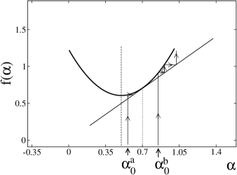
Figure 1: Graphical analysis of the representations of the GHA for $f(\alpha)=2.5\alpha^{2}-2.5\alpha+1.225$ ($\Delta=0$). Note that there is one fixed point $\alpha^{*}=0.7$ (vertical doted line) within the region under analysis, $\alpha>-q/(2t)=0.5$ (vertical dashed line). Note also that $\alpha_{0}^{a}$ is a starting point whose future iterations tend to the fixed point $\alpha^{*}=0.7$ while $\alpha_{0}^{b}$ is a starting point whose future iterations go to infinity. These two different choices correspond to infinite-dimensional representations for the GHA while the choice $\alpha_{0}=\alpha^{*}$ correspond to a one-dimensional representation of the algebra.

3 Generalised $sl(2)$ algebra

In a similar way that was constructed the GHA, a generalisation of the $sl(2)$ algebra was introduced where in the commutation relations of their generators there is a characteristic function $g$ of one of their own generators [14]. This new algebraic structure is constructed by the following relations among their generators

$$J_{0}\,J_{-} = J_{-}\,g(J_{0})$$ (8)

$$J_{+}\,J_{0} = g(J_{0})J_{+}$$ (9)

$$\left[J_{+},J_{-}\right] = J_{0}(J_{0}+1)-g(J_{0})(g(J_{0})+1)$$ (10)

where $J_{-}=(J_{+})^{\dagger}$, $J_{0}^{\,\dagger}=J_{0}$ and $g(J_{0})$ is any analytical function in $J_{0}$ [14]. Using the eqs.(8-10) it was shown that the operator

$$\widehat{C}\equiv\frac{1}{2}\left\{{J_{+}\,J_{-}+J_{-}}\,J_{+}+J_{0}(J_{0}+1)+g(J_{0})(g(J_{0})+1)\right\}$$ (11)

is the casimir operator of the algebra. If we chose the function $g(J_{0})=J_{0}-1$ we can easily see that the relations (8-10) become the widely known commutation relations of the $sl(2)$ algebra [21]. Departuring from this special case for the characteristic function $g$ we obtain different algebraic structures that generalise the $sl(2)$ algebra in the sense that we can recover the standard $sl(2)$ algebra when $g(J_{0})\rightarrow J_{0}-1$. For instance, considering $g(J_{0})=qJ_{0}-1$, the G-$sl(2)$ algebra corresponds to the $sl_{q}(2)$ algebra, which in the limit $q\rightarrow 1$ turns into the standard $sl(2)$ algebra [14]. In the non-linear case, the algebraic structure become more general than the $sl(2)$ and $sl_{q}(2)$ algebras. Is in this non-linear case for the characteristic function $g$ that we are going to exhibit a class of generalised JS maps that realises the generators of the G-$sl(2)$ algebra in terms of the generators of the GHA with a non-linear characteristic function $f$.

Seeking for the representations of the G-$sl(2)$ algebra, we suppose [14] that exists a highest weight state of the representation $|\alpha_{j};j\rangle$ defined as

$$J_{+}\,|\alpha_{j};j\rangle\equiv 0$$ (12)

whose $J_{0}$ eigenvalue is $\alpha_{j}$, i.e. $J_{0}|\alpha_{j};j\rangle=\alpha_{j}|\alpha_{j};j\rangle$, where $\alpha_{j}$ is a real number and $j$ is a natural number. Applying sucessively $J_{-}$ on this highest weight state, we have different $J_{0}$ eigenstates that form a basis of the Fock space. The representation of the algebra is obtained by the application of the algebra generators on this basis. For a general characteristic function $g$ we obtain, for $m=0,1,...,2j$, the following representation of the algebra

$$J_{0}\,\,|\alpha_{j};j-m\rangle = \alpha_{j-m}|\alpha_{j};j-m\rangle$$ (13)

$$J_{+}\,\,|\alpha_{j};j-m\rangle = \widehat{M}_{m-1}|\alpha_{j};j-m+1\rangle$$ (14)

$$J_{-}\,\,|\alpha_{j};j-m\rangle = \widehat{M}_{m}|\alpha_{j};j-m-1\rangle$$ (15)

$$\widehat{C}|\alpha_{j};j-m\rangle = \alpha_{j}(\alpha_{j}+1)\,|\alpha_{j};j-m\rangle$$ (16)

where by hypothesis the function $g$ and the initial value $\alpha_{j}$ satisfy $\alpha_{j}>g^{(m)}(\alpha_{j})$, where $g^{(m)}(\alpha_{j})$ is the $m$-th iteration of $\alpha_{j}$ through $g$, $\widehat{M}^{2}_{m}=(\alpha_{j}-\alpha_{j-m-1})(\alpha_{j}+\alpha_{j-m-1}+1)=\alpha_{j}(\alpha_{j}+1)-\alpha_{j-m-1}(\alpha_{j-m-1}+1)$ and $\alpha_{j-m}=g^{(m)}(\alpha_{j})=g(\alpha_{j-m+1})$ for a integer $m\geq 1$ [14].

Hereafter we are going to discuss the finite- and infinite-dimensional representations of the algebra described by the commutation relations (8-10), where we will consider a non-linear charactereristc function $g(\alpha)=t^{{}^{\prime}}\alpha^{2}+q^{{}^{\prime}}\alpha-s^{{}^{\prime}}$ with $t^{{}^{\prime}}<0$ and under the restriction $\alpha<-q^{{}^{\prime}}/(2t^{{}^{\prime}})$ in order to consider inversible functions.

For the finite-dimensional representations, since each representation is constructed from the highest weight state, we can find out two different constraints for $\alpha_{j}$ such that the eq.(15) is identically null, i.e. for a $d$-dimensional representation $\widehat{M}_{d+1}=0$, given by

$$\alpha_{j}=\alpha_{j-d}$$ (17)

and

$$\alpha_{j}+\alpha_{j-d}+1=0.$$ (18)

Otherwise, the dimension of the representations will be infinite.

The solutions of the eq.(17) can be studied by analysis of the stability of the attractors of $g$ and their composed functions. So, we are going to focus on the graphical analysis of the stability of the fixed points $\overline{\alpha^{*}}$, attractors of period 1, solutions of the equation $\overline{\alpha^{*}}=g(\overline{\alpha^{*}})$. For simplicity, we will consider the case $\Delta=(q^{{}^{\prime}}-1)^{2}+4t^{{}^{\prime}}s^{{}^{\prime}}=0$.

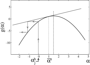
Figure 2: Graphical analysis of the representations of the generalised $sl(2)$ algebra for $g(\alpha)=-\alpha^{2}+3\alpha-1$ ($\Delta=0$). Note that there is one fixed point $\overline{\alpha^{*}}=1$ and there are two different regions that correspond to two different asymptotic behaviours to the $J_{0}$ eigenvalues associated with infinite-dimensional representations of the algebra. In the figure, we exhibit the iteration of $\alpha^{b}_{j}$ whose future iterations tend to $-\infty$. Note also that the one-dimensional representation can be obtained for the choice $\alpha_{j}=\overline{\alpha^{*}}$.

In this case $g$ presents a fixed point $\overline{\alpha^{*}}=(1-q^{{}^{\prime}})/2t^{{}^{\prime}}$; for $\alpha_{j}=\overline{\alpha^{*}}$ the algebra has a one-dimensional representation ($d=1$) since $\alpha_{j}=\alpha_{j-1}=\overline{\alpha^{*}}$. Apart from this finite-dimensional representation, the algebra has infinite-dimensional representations associated with the following regions of $\alpha_{j}$: ($a$) $\overline{\alpha^{*}}<\alpha_{j}<-q^{{}^{\prime}}/(2t^{{}^{\prime}})$ and ($b$) $-\infty<\alpha_{j}<\overline{\alpha^{*}}$. In the case $(a)$ the $J_{0}$ eigenvalues, $g^{(m)}(\alpha_{j})$, go to the asymptotic value $\overline{\alpha^{*}}$ while in the region $(b)$ go to $-\infty$. In the figure 2 we plot the functions $g(\alpha)=-\alpha^{2}+3\alpha-1$ and $y=\alpha$ versus $\alpha$ and exhibit the interations of the $\alpha_{j}^{b}=-0.05$. The vertical doted line corresponds to the fixed point $\overline{\alpha^{*}}=1$ and the vertical dashed line corresponds to $\alpha=-q^{{}^{\prime}}/(2t^{{}^{\prime}})=1.5$.

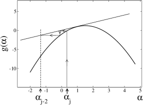
Figure 3: Graphical analysis of the representation of the generalised $sl(2)$ algebra for $g(\alpha)=-\alpha^{2}+3\alpha-1$ ($\Delta=0$). Note that there is a finite-dimensional representation associated with the cut condition equation, $\alpha_{j-2}=-\alpha_{j}-1$. In this plot we show a two-dimensional representation ($j=1/2$) with $\alpha_{j}=0.33479$. There is also another two-dimensional representation of the algebra for $\alpha_{j}=2.9228$, but this value is out of the region, $\alpha<-q^{{}^{\prime}}/(2t^{{}^{\prime}})=1.5$, in analysis.

It is important to say that the algebra has infinite-dimensional representations if we choose an $\alpha_{j}$ within the allowed regions and if the cut condition equation (18) is not satisfied for any future iteration. As stated before, the cut condition equation (18) corresponds to the $d$-dimensional representations of the algebra. For instance, using $t^{{}^{\prime}}=-1$, $q=3$ and $s^{{}^{\prime}}=1$, that corresponds to $\Delta=0$, and selecting the representation $j=1/2$ ($d=2$) we obtain $\alpha_{j}=0.33479$ and $\alpha_{j}=2.9228$ as solutions of the eq.(18). So, in order to obtain two representations of dimension $d=2$ of the algebra, we can choose one or the other solution for $\alpha_{j}$.

An example of this finite dimensional case is showed in figure 3 where we plot the function $g(\alpha)=-\alpha+3\alpha-1$ and $y=\alpha$ versus $\alpha$ and where we select the two-dimensional representation $d=2$ ($j=1/2$) choosing $\alpha_{j}=0.33479$. We also plot the vertical doted line $\alpha_{j-2}=\alpha_{j}-1=-1.33479$, which represents the cut condition equation (18). Since $\alpha_{j}=2.9228$ is out of the region in analysis, $\alpha<-q^{{}^{\prime}}/(2t)=1.5$, we did not exhibit the interations of this solution.

4 A class of generalised Jordan-Schwinger maps

First of all, we consider the algebra of two independent (uncoupled) deformed oscillators which we call the $1$-type and the $2$-type. We assume that the commutation relations of the generators of their individual algebras satisfy the relations (1-3) for a general analytical function $f$. As we saw in section 2, these algebras have a general representation given by

$$H_{1}|n_{1},n_{2}\rangle = f^{(n_{1})}(\alpha_{0})|n_{1},n_{2}\rangle\;\>$$ (19)

$$A^{\dagger}_{1}|n_{1},n_{2}\rangle = M_{n_{1}}|n_{1}+1,n_{2}\rangle$$ (20)

$$A_{1}|n_{1},n_{2}\rangle = M_{n_{1}-1}|n_{1}-1,n_{2}\rangle$$ (21)

where $M^{2}_{n_{1}-1}=f^{(n_{1})}(\alpha_{0})-\alpha_{0}$, $n_{i}=1,2,3,....$ for $i=1,2$ and $|n_{1},n_{2}\rangle\equiv|n_{1}\rangle\otimes|n_{2}\rangle$, where $\otimes$ is the tensorial product. Analogously $H_{2},A^{\dagger}_{2}$ and $A_{2}$ act on the second entry of $|n_{1},n_{2}\rangle$. Here we consider that $H_{1}$ and $H_{2}$ have vacuum eigenstates with same eigenvalues, i.e. $\alpha^{(1)}_{0}=\alpha^{(2)}_{0}\equiv\alpha_{0}$, where $H_{1}|0,0\rangle=\alpha^{(1)}_{0}|0,0\rangle$ and $H_{2}|0,0\rangle=\alpha^{(2)}_{0}|0,0\rangle$.

Starting from the vacuum eigenstate $|0,0\rangle$ we can construct different eigenstates of the two deformed oscillators given by

$$|n_{1},n_{2}\rangle=\frac{(A^{\dagger}_{1})^{n_{1}}(A^{\dagger}_{2})^{n_{2}}}{M^{n_{1}+n_{2}}_{0}\sqrt{\left[n_{1}\right]_{f}!\left[n_{2}\right]_{f}!}}|0,0\rangle$$ (22)

where the generalised Gauss number of $m$, denoted by $\left[m\right]_{f}$, for a general function $f$, is defined as [13]

$$\left[m\right]_{f}\equiv\frac{M^{2}_{m-1}}{M^{2}_{0}}=\frac{f^{(m)}(\alpha_{0})-\alpha_{0}}{f(\alpha_{0})-\alpha_{0}}$$ (23)

and

$$\left[m\right]_{f}!\equiv\left[m\right]_{f}\left[m-1\right]_{f}...\left[1\right]_{f}.$$ (24)

The aim herein is to exhibit a JS map that connects two independent GHA, with the same non-linear characteristic function $f$, to the G-$sl(2)$ algebra with a non-linear characteristic function $g$. Similarly to the standard JS map, we introduce the following map

$$S_{z} \equiv G(N_{1},N_{2})$$ (25)

$$S_{+} \equiv F(N_{1},N_{2})A^{\dagger}_{1}A_{2}$$ (26)

$$S_{-} \equiv A^{\dagger}_{2}A_{1}F(N_{1},N_{2}),$$ (27)

where $N_{1}$ and $N_{2}$ are the number operators defined as

$$N_{1}|n_{1},n_{2}\rangle=n_{1}|n_{1},n_{2}\rangle$$ (28)

$$N_{2}|n_{1},n_{2}\rangle=n_{2}|n_{1},n_{2}\rangle$$ (29)

and the functional $F$ and $G$ have the following forms

$$F(N_{1},N_{2})\equiv\frac{\sqrt{-Q_{2}\left[j+1-\frac{N_{1}-N_{2}}{2}\right]_{g}\left(2\alpha_{j}+1+Q_{2}\left[j+1-\frac{N_{1}-N_{2}}{2}\right]_{g}\right)}}{M^{2}_{0}\sqrt{\left[j+1-\frac{N_{1}-N_{2}}{2}\right]_{f}\left[j+\frac{N_{1}-N_{2}}{2}\right]_{f}}}$$ (30)

and

$$G(N_{1},N_{2})\equiv\alpha_{j}+Q_{2}\left[j-\frac{N_{1}-N_{2}}{2}\right]_{g}$$ (31)

where $Q_{2}=g(\alpha_{j})-\alpha_{j}$, $\left[m\right]_{f}=\frac{f^{m}(\alpha_{0})-\alpha_{0}}{f(\alpha_{0})-\alpha_{0}}$ and $\left[m\right]_{g}=\frac{g^{m}(\alpha_{j})-\alpha_{j}}{g(\alpha_{j})-\alpha_{j}}$ $\forall m$ positive integer, where $f$ and $g$ are general analytical functions. We can notice that for $f(x)=x+1$ and $g(x)=x-1$ the generalised JS map recovers the form of the standard JS map [21] since $G(N_{1},N_{2})\rightarrow\frac{N_{1}-N_{2}}{2}$ and $F(N_{1},N_{2})\rightarrow 1$.

As it will become clear later, the operator

$$S^{2}\equiv\frac{1}{2}\left[S_{+}S_{-}+S_{-}S_{+}+S_{z}(S_{z}+1)+g(S_{z})(g(S_{z})+1)\right]$$ (32)

is the Casimir operator of the algebra generated by $S_{z}$, $S_{+}$ and $S_{-}$.

If we identify

$$n_{1}\rightarrow j+m\Longrightarrow j=\frac{n_{1}+n_{2}}{2}$$ (33)

$$n_{2}\rightarrow j-m\Longrightarrow m=\frac{n_{1}-n_{2}}{2}$$ (34)

we can easily check from eq.(22), that the more general eigenstate of the operator $S_{z}$ is written as

$$|j,m\rangle=\frac{(A^{\dagger}_{1})^{j+m}(A^{\dagger}_{2})^{j-m}}{M^{2j}_{0}\sqrt{\left[j+m\right]_{f}!\left[j-m\right]_{f}!}}|0,0\rangle$$ (35)

where $m=-j,-j+1,...,0,...,j-1,j$. Without loss of generality we identify $m\rightarrow j-m$ and denote $|j,j-m\rangle\equiv|\alpha_{j},j-m\rangle$ where $m=0,1,2,...,2j$. The representation of the algebra is fixed by $S_{z}$, $S_{+}$ and $S_{-}$ obtained by the action of these operators on the $S_{z}$ eigenstates, $|\alpha_{j},j-m\rangle$, given by:

$$S_{z}|\alpha_{j},j-m\rangle=(\alpha_{j}+Q_{2}\left[m\right]_{g})|\alpha_{j},j-m\rangle$$ (36)

$$S_{+}|\alpha_{j},j-m\rangle=\sqrt{-Q_{2}\left[m\right]_{g}(2\alpha_{j}+1+Q_{2}\left[m\right]_{g})}\,\,|\alpha_{j},j-m+1\rangle$$ (37)

$$S_{-}|\alpha_{j},j-m\rangle=\sqrt{-Q_{2}\left[m+1\right]_{g}(2\alpha_{j}+1+Q_{2}\left[m+1\right]_{g})}\,\,|\alpha_{j},j-m-1\rangle$$ (38)

$$S^{2}|\alpha_{j},j-m\rangle=\alpha_{j}(\alpha_{j}+1)|\alpha_{j},j-m\rangle,$$ (39)

valid for general analytical functions $f$ and $g$, where we can see that $S^{2}$ is the Casimir operator of the algebra. It is very important to stress that this representation (36-39) is valid for all $m=0,1,2,...,2j$. So, the generalised JS map (25-27) is well defined.

Once presented the generalised JS map, eqs.(25-27), we can readily prove that this map in fact realises the G-$sl(2)$ algebra. For this, we will show that the operators $J_{0}$, $J_{+}$,$J_{-}$ and $\widehat{C}$ act on the $2j+1$ states of the representation of the G-$sl(2)$ algebra exactly as the operators $S_{z}$, $S_{+}$, $S_{-}$ and $S^{2}$, defined in eqs.(25-27,32), act on the $2j+1$ states of their own representation. In order to check this, we use $\left[m\right]_{g}=\frac{g^{m}(\alpha_{j})-\alpha_{j}}{g(\alpha_{j})-\alpha_{j}}=\frac{\alpha_{j-m}-\alpha_{j}}{Q_{2}}$ and $\alpha_{j-m}=g^{m}(\alpha_{j})$. So, we can rewrite the representation of the G-$sl(2)$ algebra (13-16) as

$$J_{0}|\alpha_{j},j-m\rangle=(\alpha_{j}+Q_{2}\left[m\right]_{g})|\alpha_{j},j-m\rangle$$ (40)

$$J_{+}|\alpha_{j},j-m\rangle=\sqrt{-Q_{2}\left[m\right]_{g}(2\alpha_{j}+1+Q_{2}\left[m\right]_{g})}\,\,|\alpha_{j},j-m+1\rangle$$ (41)

$$J_{-}|\alpha_{j},j-m\rangle=\sqrt{-Q_{2}\left[m+1\right]_{g}(2\alpha_{j}+1+Q_{2}\left[m+1\right]_{g})}\,\,|\alpha_{j},j-m-1\rangle$$ (42)

$$\widehat{C}|\alpha_{j},j-m\rangle=\alpha_{j}(\alpha_{j}+1)|\alpha_{j},j-m\rangle$$ (43)

and our proof is complete.

In (25-27) we see that the generators of the G-$sl(2)$ algebra are written in terms of the generators of the GHA. Since there is an interpretation for the GHA in terms of composite particles, the generalised JS map allows us to carry out this assertion in such away that the G-$sl(2)$ algebra could be related to composite particles with angular momentum. So, the generalised JS map (25-27) can be an importante tool that gets up the physical interpretation for the G-$sl(2)$ algebra, which certainly will describe phenomenologicaly several important features of systems formed by composite particles with angular momentum.

Now, let us discuss the most simple non-linear case where the characteristic functions $f$ and $g$ are polynomial quadratic ones. In this case, we would like to stress that it is possible to simplify the generalised JS map by special choices of the functions $f$ and $g$. So, if we assume $f(\alpha_{0})=t\alpha_{0}^{2}+q\alpha_{0}+1$, $g(\alpha_{j})=-t\alpha_{j}^{2}+q\alpha_{j}-1$ and $\alpha_{j}=-\alpha_{0}$ we can see that $-Q_{2}\left[m\right]_{g}=M^{2}_{0}\left[m\right]_{f}$ $\forall m$ integer, in such way that the expression for the functional $F$ leads to

$$F(N_{1},N_{2}) = \frac{\sqrt{2\alpha_{j}+1+Q_{2}\left[j+1-\frac{N_{1}-N_{2}}{2}\right]}}{\sqrt{-Q_{2}\left[j+\frac{N_{1}-N_{2}}{2}\right]}}$$ (44)

where, hereafter, $\left[m\right]=\frac{g^{m}(\alpha_{j})-\alpha_{j}}{g(\alpha_{j})-\alpha_{j}}$ for the above defined quadratic function $g$. Note also that the representation (36-39) is invariant.

The next step is to check if the above simplified assumptions for $f$, $g$ and for the parameters $\alpha_{0}$ and $\alpha_{j}$ are possible in the GHA and in the G-$sl(2)$ algebra.

As stated in sections 2 and 3, the representations of each algebra can be studied through the analyses of the stability of the attractors of $f$ (or $g$) and their composed functions. Similarly discussed in sections 2 and 3, we will consider the characteristic functions $f(\alpha)=t\alpha^{2}+q\alpha+1$ with $\alpha_{0}>-q/{2t}$ and $g(\alpha)=-t\alpha^{2}+q\alpha-1$ with $\alpha_{j}<q/(2t)$.

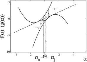
Figure 4: Graphical analyses of the representations of the G-$sl(2)$ algebra and of the GHA for $f(\alpha)=\alpha^{2}+3\alpha+1$ and $g(\alpha)=-\alpha^{2}+3\alpha-1$ ($\Delta=0$). Note that there is one fixed point $\alpha^{*}=-1$ and $\overline{\alpha^{*}}=1$ for $f$ and $g$, respectively. Note also that it is possible to choose $\alpha_{0}$ as a lowest weight of the GHA representation that implies $\alpha_{j}=-\alpha_{0}$ being the highest weight of the representation of the G-$sl(2)$ algebra. In this figure we show the case $\alpha_{0}=-0.15$ and $\alpha_{j}=-\alpha_{0}=0.15$.

We see that in the GHA, for $\Delta=(q-1)^{2}-4t=0$, the regions for $\alpha_{0}$ associated with infinite-dimensional representations are given by: $(i)$ $-q/(2t)<\alpha_{0}<\alpha^{*}$ and $(ii)$ $\alpha^{*}<\alpha_{0}<\infty$ where $f^{{}^{\prime}}(-q/(2t))=0$ and $\alpha^{*}$ is the fixed point of $f$. On the other hand, in the G-$sl(2)$ algebra, there are also regions for $\alpha_{j}$ where we can find a highest weight state and where the algebra presents infinite-dimensional representations. These regions are: ($a$) $\overline{\alpha^{*}}<\alpha_{j}<q/(2t)$ and ($b$) $-\infty<\alpha_{j}<\overline{\alpha^{*}}$, where $g^{{}^{\prime}}(q/(2t))=0$ and $\overline{\alpha^{*}}$ is the fixed point of $g$. From the allowed regions for $\alpha_{0}$ we can see that each value within it corresponds to a value $\alpha_{j}=-\alpha_{0}$ within the allowed regions for $\alpha_{j}$ since

$$\overline{\alpha^{*}}=-\alpha^{*}.$$ (45)

An example of this case is shown in figure 4 where we plot the functions $f(\alpha)=\alpha^{2}+3\alpha+1$, $g(\alpha)=-\alpha^{2}+3\alpha-1$ and $y=\alpha$ versus $\alpha$. In this figure we exhibit the iterations of $\alpha_{0}=-0.15$ and $\alpha_{j}=-\alpha_{0}=0.15$. The algebras can present also a one-dimensional representations for $\alpha_{0}=\alpha^{*}$ and $\alpha_{j}=-\alpha_{0}=\overline{\alpha^{*}}$.

Now we address our atention to discuss the finite-dimensional representations of the G-$sl(2)$ algebra coming from the cut condition equation

$$\alpha_{j}+\alpha_{j-d}+1=0.$$ (46)

As showed in section 3, for the characteristic function $g(\alpha)=-\alpha^{2}+3\alpha-1$, in order to obtain a two-dimensional representation of the G-$sl(2)$ algebra we can choose $\alpha_{j}=0.33479$ or $\alpha_{j}=2.9228$. In figure 3 we have showed the iterations for the choice $\alpha_{j}=0.33479$. We can see that the value $\alpha_{0}=-\alpha_{j}=-0.33479$ is within the allowed region for $\alpha_{0}$, $\alpha^{*}<\alpha_{0}<\infty$, that corresponds to an infinite-dimensional representation for the GHA for $f(\alpha)=\alpha^{2}+3\alpha+1$.

Finaly, we argue that for any general non-linear characteristic functions $f$ and $g$, we can always choose, for a given function $f(\alpha_{0})=\sum_{i=1}^{n}a_{i}\,(\alpha_{0})^{i}+1$, a function $g(\alpha_{j})=\sum_{i=1}^{n}\overline{a_{i}}\,(\alpha_{j})^{i}-1$ where $\overline{a_{i}}=-a_{i}$, if $i$ is even, and $\alpha_{j}=-\alpha_{0}$ in such away that $-Q_{2}\left[m\right]_{g}=M^{2}_{0}\left[m\right]_{f}$ $\forall m$ integer. So, we can simplify the functional $F$ in order to turn the generalised JS map more simple. Of course, given the algebraic parameters we must be careful and to find out the allowed regions for $\alpha_{0}$ and $\alpha_{j}$.

5 Conclusion

We introduced a class of generalised JS maps which realises the generators of the G-$sl(2)$ algebra with a non-linear characteristic function $g$, in terms of the generators of two independent GHA with a non-linear characteristic function $f$. We shown that it was necessary to generalise the standard JS map, putting not only a quadratic form of the ladder operators present in each independent GHA, but also joining a functional of the number operators. We have shown also that this generalised JS map has a simple and compact form which includes the standard JS map as a particular case.

The need of such generalisation come from the fact that these two classes of generalisations of the Heisenberg and $sl(2)$ algebras, contain, in essence, more general algebraic structures than their deformed and non-deformed algebras [14]. In spite of this, we see that is always possible to simplify the generalised JS map by special choices of the characteristic functions that are present in each generalised algebra. Of course, this statement have to be analysed with more physical accurency as discussed at the end of the previous section.

Finaly, we argue that since there are interpretations in terms of composite particles for the GHA, the generalised JS map presented in this work is a bridge which suggests a physical interpreation for the G-$sl(2)$ algebra in terms of composite particles with angular momentum. Obviously, a investigation of this assertion is highly desirable in order to check this interpretation.

References

References

- [1] Palev T D 1971 Comptes Rendus de l’Academie Bulgare des Sciences 24 565. Palev T D 1999 Mod. Phys. Lett. A 4 299-306.
- [2] Jordan P 1935 Zeit. Phys 94 531.
- [3] Schwinger J 1965 Quantum theory of angular momentum (New York: Academic) ed L C Biedenharn and H Van Dam.
- [4] Man’ko V I, Marmo G ,Vitale P and Zaccaria F 1994 Int. J. Mod. Phys. A 9 5541-5561 (Preprint hep-th/9310053)
- [5] Mota R D, Xicotencatt M A and Granados V D 2004 J. Phys. A: Math. Gen. 37 (7) 2835-2842 Mota R D , Xicotencatt M A and Granados V D 2004 Canadian J. Phys. 82 (10) 767-773. Marmo G, Simoni A and Ventriglia F 2001 Reports Math. Phys. 48 (1-2) 149-157. Banerjee R, Chakraborty B 1995 Nuclear Phys. B 449 (1-2) 317-346. Defalco L, Migmani R and Scipioni R 1995 Phys. Lett. A 201 (1) 9-11.
- [6] Klein A and Marshalek E R 1991 Rev. Mod. Phys. 63 375.
- [7] Ruan D, Li Y S and Sun H Z 2007 Comm. Theor. Phys 47 (3) 529-534. Kumar V S, Bambah B A and Jagannathan R 2002 Mod. Phys. Lett. A 17 (24) 1559-1566. Daskaloyannis C, Kanakoglou K and Tsohantjis I 2000 J. Math. Phys. 41 (2) 652-660 . Zhedanov A S 1992 J. Phys. A: Math. Gen. 25 L713-L717.
- [8] Cho K H, Park S U 1995 J. Phys. A 28 1005-1016 (Preprint hep-th/9406084). Cahn R N 1984 Semi-Simple Lie Algebras and Their Representations (Addison-Wesley Publishing Company, The Advanced Book Program).
- [9] Biedenharn L C 1989 J. Phys. A 22 L873.
- [10] Mac Farlane A J 1989 J. Phys. A 22 4581.
- [11] Curado E M F and Rego-Monteiro M A 2001 Physica A 295 268-275.
- [12] See for instance (this is not a complete list) Sviratcheva K D, Bahri C, Georgieva A I, Draayer J P 2004 Phys. Rev. Lett. 93 152501-1 Gu S J , Lin H Q and Li Y Q 2003 Phys. Rev. A 68 042330. Bonatsos D, Kotsos B A, Raychev P P, Terziev D A 2002 Phys. Rev. C 66 054306. Faddeev L D, Sklyanin E K and Takhajan L A 1979 Theor. Math. Phys. 40 194. Faddeev L D 1982 Les Houches Seession XXXIX (Amsterdam: Elsevier) p.563.
- [13] Curado E M F and Rego-Monteiro M A 2001 J. Phys. A: Math. Gen. 34 3253-3264.
- [14] Curado E M F and Rego-Monteiro M A 2002 Phys. Lett. A 300 205-212.
- [15] Bezerra V B, Curado E M F and Rego-Monteiro M A 2002 Phys. Rev. D 65 065020.
- [16] Bezerra V B, Curado E M F and Rego-Monteiro M A 2002 Phys. Rev. D 66 085013.
- [17] Ribeiro-Silva C I and Oliveira-Neto N M 2004 Preprint hep-ph/0409267.
- [18] de Souza J, Oliveira-Neto N M and Ribeiro-Silva C I 2006 Eur. Phys. J. D 40 (2) 205-210.
- [19] Oliveira-Neto N M, Curado E M F, Nobre F D and Rego-Monteiro M A 2007 J. Phys. B: At. Mol. Opt. Phys. 40 1975-1989. Oliveira-Neto N M, Curado E M F, Nobre F D and Rego-Monteiro M A 2004 Physica A 344 573.
- [20] Curado E M F, Rego-Monteiro M A and Nazareno H N 2001 Phys. Rev. A 64 012105 (Preprint hep-th/0012244).
- [21] Sakurai J J 1994 Modern Quantum Mechanics (Addison-Wesley Publishing Company, Revised Edition).