INSTITUT NATIONAL DE RECHERCHE EN INFORMATIQUE ET EN AUTOMATIQUE

GCP: Gossip-based Code Propagation for Large-scale Mobile Wireless Sensor Networks
Yann Busnel — Marin Bertier — Eric Fleury — Anne-Marie KermarrecN° 6251
Juin 2007

Abstract: Wireless sensor networks (WSN) have recently received an increasing interest. They are now expected to be deployed for long periods of time, thus requiring software updates. Updating the software code automatically on a huge number of sensors is a tremendous task, as ”by hand” updates can obviously not be considered, especially when all participating sensors are embedded on mobile entities.

In this paper, we investigate an approach to automatically update software in mobile sensor-based application when no localization mechanism is available. We leverage the peer-to-peer cooperation paradigm to achieve a good trade-off between reliability and scalability of code propagation. More specifically, we present the design and evaluation of GCP (Gossip-based Code Propagation), a distributed software update algorithm for mobile wireless sensor networks. GCP relies on two different mechanisms (piggy-backing and forwarding control) to improve significantly the load balance without sacrificing on the propagation speed. We compare GCP against traditional dissemination approaches. Simulation results based on both synthetic and realistic workloads show that GCP achieves a good convergence speed while balancing the load evenly between sensors.

Key-words: Wireless sensor network, mobile computing, large scale, diffusion, software update, peer-to-peer algorithm, simulation

GCP: Mise à jour épidémique de logiciels pour les réseaux de capteurs mobiles, larges échelles

Résumé : GCP est un systeme de mise à jour de code automatique pour réseaux de capteurs mobiles, utilisant le concept de diffusion épidémique développés dans le cadre de réseaux filaires.
Ce rapport présente la conception et l’évaluation de GCP (Gossip-based Code Propagation), protocole proposé dans le cadre de ces travaux de recherches.

Celui-ci est évalué par comparaison avec des algorithmes traditionnels de dissemination de données. Les résultats de simulations sont fondés à la fois sur des traces réelles et générées, permettant de montrer l’efficacité de GCP tant dans la vitesse de propagation que dans l’équilibrage des charges sur le réseau.

Mots-clés : réseaux de capteurs, informatique mobile, large échelle, diffusion, mise à jour de code, systèmes pair-à-pair, simulation

1 Introduction

Recently, compact devices, called micro-electro mechanical systems (MEMS), have appeared. Such devices combine small size, low cost, adaptability, low power consumption, large scale and self-organization. Equipped with wireless communication capability, such appliances (called mote node or sensor) together form a wireless sensor network (WSN). Due to their tiny size, sensors possess slim resources in term of memory, CPU, energy, etc. [1, 16].

The increasing interest in WSNs is fundamentally due to their reliability, accuracy, flexibility, cost effectiveness and ease of deployment characteristics. Such WSNs can be deployed for monitoring purposes for example. For example we can cite Ecosystem monitoring, Military (battlefield surveillance, enemy tracking, …), Biomedical and health monitoring (cancer detector, artificial retina, organ monitor, …), Home (childhood education, smart home/office environment, …).

Sensors may be deployed both in static and dynamic environments. They are usually deployed for a long period of time, during which the software may require updates. While efficient solutions to software update may be deployed in fixed WSNs, this is far more complex when sensors are embedded on mobile entities such as people. In this paper, we consider this latter setting, namely a WSN deployed over a group of people.

Given the potentially large number of participating sensors in WSN and their limited resources, it is crucial to use fully decentralized solutions and to balance the load as evenly as possible between participating sensors. In that context, we investigate the use of the P2P communication paradigm which turns out to be a relevant candidate in this context. Considering similarities between these two systems, Section 2 investigates the relevance of adapting the P2P paradigm to mobile WSN. Using epidemic-based dissemination, we introduce a greedy protocol (GCP: Gossip-based Code Propagation) balancing the dissemination load without increasing diffusion time. GCP relies on piggy-backing to save up energy and forwarding control to balance the load among the nodes.

Code propagation (or reprogramming service) has a lot in common with broadcast and data dissemination [5, 8] with an additional main-constraint. In broadcast, each message sent before a node arrival can be ignored by this node. In software update protocols, each new node in the network has to be informed of the existence of the software’s latest version as soon as possible to be operational.

This paper is organized as follows. Section 2 presents the P2P paradigm and more specifically the epidemic principle. Section 3 introduces the GCP algorithm and alternative approaches. We compared GCP with classical approaches by simulation and depict the results in Section 4. Finally, Section 5 introduces a short state of art of the different domains cited above before concluding in Section 6.

2 Applying P2P algorithms to mobile WSN

Classical peer-to-peer systems are composed of millions of Personal Computers connected together by a wired network and as opposed to sensor networks are not limited by node capacity, communication range or system size (see Table 1). In this section we promote the idea that sensor networks and peer-to-peer systems are similar enough so that P2P solutions can be seriously considered in the context of WSNs.

	Peer to peer systems	Sensor networks
Similarities
System size	Millions	Thousands
Dynamicity	Connection/disconnection	Mobility
	Failure	Failure (low power)
Differences
Resource	Plentiful	Tiny
Potential neighbourhood	Chosen among the whole system	Impose
Connectivity	Persistent	Temporary

Table 1: Similarity and divergence between P2P systems and WSNs

2.1 Peer-to-Peer vs. mobile WSN

On one hand, sensors and personal computers have incomparable resources: PCs have large resources in terms of CPU, storage while sensors are very limited; sensors have strong energy constraints, limiting their capability to communicate. On the other hand, due to the node’s resources compared to the size of the system, no entity is able to manage the entire network in both systems. Every application designed for both networks requires a strong cooperation between entities to be able to manage the network and to take advantage of the entire network. Peer to peer solutions heavily rely on such collaboration.

The peer to peer communication paradigm has been clearly identified as a key to scalability in wired systems. In a P2P system, each node may act both as a client and a server, and knows only few other nodes. Each node is logically connected to a subset of participating nodes forming a logical overlay over the physical network. With this local knowledge, the resource aggregation and the load are evenly balanced between all peers in the systems. Central points of failures disappear as well as associated performance bottlenecks [3, 21].

In a sensor network, a node is able to communicate only with a subset of the network within its communication range and has to opportunity to “choose”its neighbours. In addition, in a mobile WSN, the neighbourhood of a node changes according to its mobility pattern. With the exception of the sensor’s energy constraint, the other differences between this two systems which have a direct impact on the algorithm behaviour is the multicast advantage of the wireless medium. When a sensor node sends a message, this message can be received by every node in its direct neighbourhood while in a wired network a message is received only by the nodes which are explicitly designated in the message.

If solutions designed for a large scale wired network can not be applied directly in a sensor network, the peer-to-peer paradigm is implicitly used in sensor networks.

2.2 Epidemic algorithms

Epidemic or gossip-based communication is well-known to provide a simple scalable efficient and reliable way to disseminate information [10]. Epidemic protocols are based on continuous information exchange between nodes. Periodically, each node in the system chooses randomly a node in its neighbourhood to exchange information about itself or its neighbourhood. One of the key results is that in a random graph, if the node’s view (set of knowing nodes, i.e. the local view of the system) is constraint to $c=O(\log(n))$, where $n$ is the size of the network, it assures that every node in the system receive a broadcast message with a probability of $e^{-e^{-c}}$.

Based on unstructured P2P overlay, gossip-based protocols can be successfully applied in WSNs. Recently, several approaches based on gossip have been proposed in the context of WSNs [12, 13, 19, 20].

The objective of this paper is to adapt such an approach to achieve efficient and reliable software dissemination in mobile WSN.

3 GCP: Introducing control in flooding as a miracle drug to mobile WSNs

In mobile wireless sensor networks, routing and broadcasting is a challenging task due to the network dynamicity. To the best of our knowledge, existing approaches do not deal with diffusion persistence (cf. Section 5).

In the following, we consider a distributed system consisting of a finite set of mobile sensor nodes which are not aware of their geographic location. The network may not be connected at any time as at a time $t$, a node can only communicate with nodes in its communication range. However, we consider that over an application duration, given that there are an infinite number of paths between two nodes, the network is eventually connected. In order to discover its neighbourhood, each node periodically broadcasts locally Hello messages, called beacon.

3.1 GCP design

Flooding paradigm is a simple way to disseminate informations. Used commonly in the network area, it consists in forwarding to everyone known a new received information. Rather than applying classical flooding algorithms having an ideal speed propagation at the price of a high energy consumption, we use the epidemic communication paradigm, proposed in the context of P2P systems. To this end, GCP is inspired from the flooding paradigm enhanced throughPiggy-Backing and Forwarding Control.

Piggy-Backing mechanism

In order to avoid unnecessary software transmissions, nodes have to be aware of the software versions hold by their neighbours. To this end, each node simply piggy-backs its own version number into beacon messages.

Forwarding Control mechanism

In order to balance the load among node and increase the overall lifetime of a system, each node sends its current software version a limited number of times. To this end, each node owns a given number of tokens, which value is a system parameter. Sending a software update is worth a token. When a node has spent all its tokens, it is not allowed to send this version of the software. This number of tokens is associated to each version. Upon receiving a new version of the software, the number of tokens is set to the default initial value. This mimics the behaviour of an epidemic protocol, where each node sends a predefined number of time a message (typically $\log(N)$, $N$ being the size of the system) [10]. Likewise, the default value of the number of tokens can be set according the order of magnitude of WSN size.

3.2 GCP algorithm

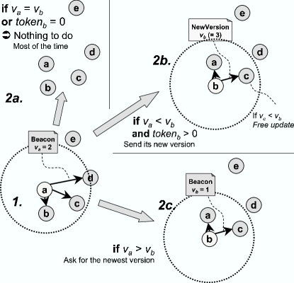
Figure 1: Summarized behaviour of GCP

Figure 1 represents the three possible different cases and the GCP behaviour.

Each node in the transmission range of $a$ receives the beacon (In Figure 1: nodes $b$, $c$ and $d$; node $e$ is out of range). A beacon message received by node $b$ is processed as follows:

1. If $b$ owns the same version as $a$ ($v_{a}=v_{b}$) due to the piggy-backing mechanism or $token_{b}=0$ due to the forwarding control mechanism, then no action is required.

2. If $b$ owns a more recent version than $a$ ($v_{a}<v_{b}$) due to the piggy-backing mechanism, and, if $b$ still holds some tokens ($token_{b}>0$) due to the forwarding control mechanism, it sends its own version to $a$ thus consuming a token ($token_{b}$–). Note that if other nodes, within the transmission range, holding an older version than $b$’s, they leverage the software update and update their own version (“free update”).

3. If $a$ owns a version newer than $b$ ($v_{a}>v_{b}$) due to the piggy-backing mechanism, the node $b$ sends immediately a beacon message in order to request a software update from $a$ while $a$ is still in its radio range.

3.3 Alternative algorithms

In order to assess the efficiency of GCP, we compare it against three other protocols, directly derived from wired networks. We briefly present those protocols in this section.

The Flooding Protocol (FP) Each time a node receives a beacon from another one, it sends its own version of the software, whether the node needs it or not. This algorithm obviously leads to load unbalance and does not take into account energy consumption. This algorithm is presented here because it provides good software propagation speed.

The Forwarding Control Protocol (FCP) This algorithm is an enhancement of the flooding protocol, using the forwarding control mechanism.

The Piggy-Backing Protocol (PBP) This last algorithm is an enhancement of the flooding algorithm, with the piggy-backing mechanism.

3.4 Protocols in Pseudo-Code

Thereafter, we introduce a formalized version of these protocols.

• $version$ and $version_{r}$ represent respectively the local and the remote version number of the software;

• $software$ and $software_{r}$ represent respectively the local and the remote binary of the software;

• $token$ represents the remaining number of tokens available on the local node;

• $initialNumberOfTokens$ represents the initial number of tokens available on the local node.

FP is presented in Figure 2.

ReceiveBeacon$(\mbox{\sc nil})$ 1 $\ignorespaces\mbox{\bf send\ }(software,version)$ ReceiveSoftware$(software_{r},version_{r})$ 1 if $version_{r}>version$ 2 then 3 $\ignorespaces\mbox{\bf updateCode\ }(software_{r})$ 4 $\ignorespaces version\leftarrow version_{r}$

Figure 2: Flooding algorithm

The GCP algorithm is presented in Figure 3. PBP has the same pseudo code without lines 2, 5 in ReceiveBeacon and without line 5 in ReceiveSoftware. FCP has the same pseudo code without lines 1, 6, 7 and 8 in ReceiveBeacon.

Each time a node receives a beacon message, it compares its own version number with the remote one. If it possesses a newer version, it sends its code to its neighbourhood. Otherwise, if it owns an older version, it sends immediately a beacon, to pull the newer version from the remote node.

When a node receives a software version, it checks this version number. If this version is a newer one, it replaces its own version by the new one and reinitializes its token number to be able to forward it.

ReceiveBeacon$(version_{r})$ 1 if $version_{r}<version$ 2 $\ignorespaces\mbox{\bf and \ }token>0$ 3 then 4 $\ignorespaces\mbox{\bf send\ }(software,version)$ 5 $\ignorespaces token\leftarrow token-1$ 6 else  if $version_{r}>version$ 7 then 8 $\ignorespaces\mbox{\bf send\ }{\rm Beacon}(version)$ ReceiveSoftware$(software_{r},version_{r})$ 1 if $version_{r}>version$ 2 then 3 $\ignorespaces\mbox{\bf updateCode\ }(software_{r})$ 4 $\ignorespaces version\leftarrow version_{r}$ 5 $\ignorespaces token\leftarrow initialNumberOfTokens$

Figure 3: Gossip-based Code Propagation algorithm

3.5 Theoretical analysis

We compare these protocols along two metrics: the software propagation speed and the number of versions sent by each node. This last metric reflects the load balance in the system. Some notations are needed and listed in the following paragraph:

• $n_{v}$ represents the number of upgrades during the WSN lifetime (how many times the software need to be updated);

• $t$ represents the number of tokens available on each node;

• $n_{nh}$ represents the average size of a node neighbourhood;

• $d$ represents the duration of the experimentation;

• $p_{b}$ represents the period of beacon emission;

• $n_{s}$ represents the network size in terms of number of nodes;

For all of the following theoretical results, each equation presents the upper bound average values. To obtain more precise results, we may take into account the diameter size, the topology and mobility model of the WSN considered.

Load balancing

For the load balancing, the analysis extracts the quantity of large message sent by each node, as software binary sending here. The following equations present the average number of software sent by one node during the whole deployment of the WSN for each algorithm:

Flooding algorithm: $$\sim \frac{d}{p_{b}}\times n_{nh}$$ (1)

$$\textrm{FCP algorithm:}(lb_{FCP}) \sim (n_{v}+1)\times t$$ (2)

$$\textrm{PBP algorithm:}(lb_{PBP}) \sim n_{v}\times(ns-1)$$ (3)

$$\textrm{GCP algorithm:}(lb_{GCP}) \sim n_{v}\times t$$ (4)

In the flooding algorithm, at each beacon reception, a node sends its own version. Equation (1) illustrates that the number of time a node sends its version is equivalent to the number of beacon sent by each node multiplied by the average number of nodes in the neighbourhood.

Both the FCP and GCP algorithms have a bound on the quantity of time a node can send its software according to $n_{v}$ and $t$. For FCP, as the version number is not communicated to neighbourhood, the first version is sent as a new one by each node. Moreover, in the FCP algorithm, tokens may be spent unnecessarily, as opposed to GCP consuming only necessary tokens thanks to the version number contained in beacon messages. We assume that $n_{s}\gg t$ to optimize balancing for token rule using algorithms in a large scale environment.

We can conclude that in the worst configuration:

$$lb_{FP}\gg lb_{PBP}\gg lb_{FCP}>lb_{GCP}$$

and in most cases:

$$lb_{FP}\gg lb_{PBP}>lb_{FCP}>lb_{GCP}$$

Propagation speed

Considering the propagation speed, the analysis extracts the propagation of a new software in the WSN. We consider the software update propagation by dividing time into software forwarding step.

We start by comparing Flooding with GCP and PBP. Let $t$ be the current step of propagation. Consider that at this step, the network is in the same state (same nodes own the newest version of the protocol, same positions of nodes and future moving, etc.) Obviously, using flooding software is equivalent to forward the software to all nodes, regardless of their need for it. At the opposite, in GCP and PBP, a node sends the newest software version only to nodes needing it. They exhibit a similar propagation speed. GCP and PBP however provides software updates “for free”. Effectively, if a node is located in the transmission range of the newest software, it will update its software without requesting it explicitly. By recurrence on $t$, Flooding algorithm propagation speed ($ps_{FP}$) is greater or equal to GCP and PBP ones (respectively $ps_{GCP}$ and $ps_{PBP}$).

Considering PBP and GCP, they are equivalent in the most common case. But, PBP may have slightly better speed propagation in case of the meeting set is unbalanced (one node is transmit the newest version most of the time i.e. this node is consuming a large part of its power). The GCP propagation speed can be slowed down as this potential node does not have enough token. However, this case does not balance the load among the network with PBP, which is one of our objective.

We are now considering GCP and FCP algorithms. By choosing an appropriate initial number of tokens, the propagation speed of these two algorithms can approach the ideal one. Furthermore, most of the time, using FCP algorithm could waste a non-negligible number of tokens by sending unnecessarily the software. The FCP algorithm propagation speed ($ps_{FCP}$) can often be strictly lower of the GCP one.

So, we can conclude that in the worst configuration:

$$sp_{FP}\geq sp_{PBP}\geq sp_{GCP}\geq sp_{FCP}$$

and most of the case:

$$sp_{FP}\geq sp_{PBP}\sim sp_{GCP}\geq sp_{FCP}$$

3.6 Summary

Figure 4 presents the relationship between each of the previous proposed algorithm. It summarizes how to transform one algorithm to obtain another one.

		FCP algorithm
	$\mathop{\vbox{\hbox{\ooalign{\raise 1.37775pt\hbox{$\hbox to94.28914pt{$\mathord{\textrm{\char 69\relax}}\mkern-6.0mu\cleaders\hbox{$\mkern-2.0mu\mathord{\textrm{\char 71\relax}}\mkern-2.0mu$}\hfill\mkern-6.0mu\mathord{\textrm{\char 71\relax}}$\hskip 0.40002pt}$}\crcr$\hbox to94.28914pt{\hskip 0.40002pt$\mathord{\textrm{\char 71\relax}}\mkern-6.0mu\cleaders\hbox{$\mkern-2.0mu\mathord{\textrm{\char 71\relax}}\mkern-2.0mu$}\hfill\mkern-6.0mu\mathord{\textrm{\char 67\relax}}$}$}}}}\limits^{\hbox{Add version in beacon}}_{\hbox{Remove version in beacon}}$		$\mathop{\vbox{\hbox{\ooalign{\raise 1.37775pt\hbox{$\hbox to81.8002pt{$\mathord{\textrm{\char 69\relax}}\mkern-6.0mu\cleaders\hbox{$\mkern-2.0mu\mathord{\textrm{\char 71\relax}}\mkern-2.0mu$}\hfill\mkern-6.0mu\mathord{\textrm{\char 71\relax}}$\hskip 0.40002pt}$}\crcr$\hbox to81.8002pt{\hskip 0.40002pt$\mathord{\textrm{\char 71\relax}}\mkern-6.0mu\cleaders\hbox{$\mkern-2.0mu\mathord{\textrm{\char 71\relax}}\mkern-2.0mu$}\hfill\mkern-6.0mu\mathord{\textrm{\char 67\relax}}$}$}}}}\limits^{\hbox{Add token number}}_{\hbox{Remove token number}}$
GCP algorithm				Flooding algorithm
	$\mathop{\vbox{\hbox{\ooalign{\raise 1.37775pt\hbox{$\hbox to81.8002pt{$\mathord{\textrm{\char 69\relax}}\mkern-6.0mu\cleaders\hbox{$\mkern-2.0mu\mathord{\textrm{\char 71\relax}}\mkern-2.0mu$}\hfill\mkern-6.0mu\mathord{\textrm{\char 71\relax}}$\hskip 0.40002pt}$}\crcr$\hbox to81.8002pt{\hskip 0.40002pt$\mathord{\textrm{\char 71\relax}}\mkern-6.0mu\cleaders\hbox{$\mkern-2.0mu\mathord{\textrm{\char 71\relax}}\mkern-2.0mu$}\hfill\mkern-6.0mu\mathord{\textrm{\char 67\relax}}$}$}}}}\limits^{\hbox{Add token number}}_{\hbox{Remove token number}}$		$\mathop{\vbox{\hbox{\ooalign{\raise 1.37775pt\hbox{$\hbox to94.28914pt{$\mathord{\textrm{\char 69\relax}}\mkern-6.0mu\cleaders\hbox{$\mkern-2.0mu\mathord{\textrm{\char 71\relax}}\mkern-2.0mu$}\hfill\mkern-6.0mu\mathord{\textrm{\char 71\relax}}$\hskip 0.40002pt}$}\crcr$\hbox to94.28914pt{\hskip 0.40002pt$\mathord{\textrm{\char 71\relax}}\mkern-6.0mu\cleaders\hbox{$\mkern-2.0mu\mathord{\textrm{\char 71\relax}}\mkern-2.0mu$}\hfill\mkern-6.0mu\mathord{\textrm{\char 67\relax}}$}$}}}}\limits^{\hbox{Add version in beacon}}_{\hbox{Remove version in beacon}}$
		PBP algorithm

Figure 4: Algorithms dependence

Table 2 summarizes the theoretical characteristics of the studied protocols. The additional local information consists in the token value included in GCP and FCP, and the beacon one is the version number included in GCP and PBP. The two latest columns are some assumptions according to load balancing and propagation speed efficiency.

	No local	No beacon	Load	Propagation
	additional	additional	balancing	speed
	information	information
Flooding Algorithm	+	+	– –	+ +
FCP Algorithm	–	+	+	–
PBP Algorithm	+	–	–	+ +
GCP Algorithm	–	–	+ +	+ +

Table 2: Algorithms comparative statement

Brown and Sreenan [2] proposed a model to compare software update algorithms in WSNs According to this model, GCP provides the following capabilities:

Propagation capabilities

Advertise

(of the existence of a new version) is provided by the piggy-backing of the version number in each beacon message;

Transfer/send

actions are provided by the MAC layer of the node;

Listen

is provided by receiving beacon message with their additional information;

Decide

is provided by the comparison of version number.

Activation capabilities

Verify

is provided by sending a MD5 signature before sending the new software version (if the software appears to be corrupted, the node resends a beacon to request another software copy);

Transfer/send

is provided by the MAC layer of the node;

As most of this kind of algorithm, GCP does not provide generation capabilities and high-level activation capabilities. It is possible to put GCP in the Deluge [7] equivalence class as it is providing the same capabilities according to the previous cite model [2].

Figure 5: Several cases of transmission range.

Figure 6: Sensor transmission probability according to $r=3$, $R=5$, and $P_{min}=0.3$.

4 Simulation results

4.1 System model

We assume that nodes can communicate only by 1-hop broadcast with nodes in their transmission range, with no collision. For a node $S$, we distinguish two ranges of transmission,$r$ and $R$, where $0<r<R$ and $\mathcal{S}_{S}(r)\subset\mathcal{S}_{S}(R)$ (cf. Figure 6). $r$ represents the radius where the transmission range is uniform, and thus messages sent by nodes separated by less than $r$ are always received (Node $A$ in Figure 6). The second range $R$ represents the radius where transmission range may be not uniform. No nodes separated by more than $R$ can receive each other transmission (Node $B$ in Figure 6). Thus, nodes separated by a distance between $r$ and $R$ may or not receive each other transmitted messages according to the Equation 5 (Node $C$ and $D$ in Figure 6, where the filled shape represented the transmission area of $S$). In Equation 5, $P_{min}$ is the transmission’s lower bound probability parameter for two nodes separated by $R$. We consider that sensor nodes have equal communication ranges. Nodes have a transmission probability defined as follows, plot in Figure 6:

$$\left\{\begin{array}[]{ll}1&\textrm{ if }d<r\\ P_{min}-\sqrt{\frac{R-d}{R-r}}\cdot\left(\frac{R-d}{R-r}-5\right)\cdot\frac{1-P_{min}}{4}&\textrm{ if }r<d<R\\ 0&\textrm{ if }d>R\\ \end{array}\right.$$ (5)

In our model, we consider mobile sensors. This mobility can be treated among different mobility models. In order to compare our results with other ones in the literature, we choose, for the synthetic workload, the widely used random way point mobility model [9].

4.2 Simulation setup

Simulator

In order to evaluate GCP, we developed SeNSim, a software implemented for mobile wireless sensor-based applications’ simulation. SeNSim is a Java software which allows the creation of mobile wireless sensor networks and analyses information dissemination under different mobility and failures scenarios. The simulator also allows the evaluation of the characteristics related to this protocol under different mobility, failures, and stimulus scenarios.

In order to simulate large scale sensor networks scenarios during a long period of time, the designed simulator is based on a discrete-event system. This software is composed of two different parts: (1) generation of synthetic workloads and (2) mobile WSN simulation.

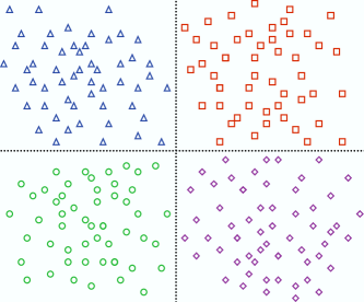
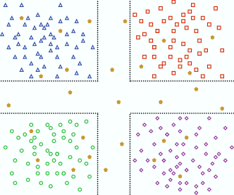
(a) Clustering scenario	(b) Socialized clustering scenario

Figure 7: Examples of synthetic scenarios with four clusters

Workloads

We evaluate different scenarios with the same set of workloads for comparison purposes. By running different algorithms on a same persistent trace, we obtain a fair comparison between each solution introduced in Section 3.

We explore the performance of GCP in various scenarios. Such scenarios exhibit different clustering and mobility patterns. Eight synthetic and one realistic scenarios have been simulated:

Synthetic

• 1 cluster scenario – One large cluster composed of 2,000 sensor nodes in a $250m\times 250m$ area.

• 1 sparse cluster scenario – The large big cluster in a wide area ($1,100m\times 1,100m$).

• 2 cluster scenario – Two 1,000 nodes’ clusters in two $800m\times 800m$ area with a $100m\times 100m$ intersection

• 2 socializing cluster scenario – Two separated 950 nodes’ clusters in two $800m\times 800m$ area. These two clusters can’t communicate with each other. We put 100 transmitters which moved in the whole area ($2,000m\times 2,000m$) to assure the connectivity.

• 4 cluster scenario – Four separated 500 nodes’ clusters in four $550m\times 550m$ areas. Connectivity is assured by the common border. These areas are set as in Figure 7(a).

• 4 socializing cluster scenario – Four separated 475 nodes’ clusters in four $550m\times 550m$ areas. These four clusters can’t communicate with each other. We put 100 transmitters which moved in the whole area ($1,300m\times 1,300m$) to assure the connectivity. These areas are set as in Figure 7(b), where transmitters are represented by a filled pentagon.

• 9 cluster scenario – Nine separated 250 nodes’ clusters in four $400m\times 400m$ areas. Connectivity is assured by the common border.

• 9 socializing cluster scenario– Nine separated 240 nodes’ clusters in four $400m\times 400m$ area. These nine clusters can’t communicate with each other. We put 90 transmitters which moved in the whole area ($1,500m\times 1,500m$) to assure the connectivity.

Realistic

• MIT Campus scenario – In order to evaluate the performance of GCP with a realistic movement behaviour, we used the mit/reality data set [6] from CRAWDAD. This data set provides captured communication, proximity, location and activity information from 100 subjects at MIT over the course of the 2004-2005 academic year.

We have used the following parameters:

• The time is discretized by millisecond.

• Each sensor node:

  • is initially randomly placed inside its defined area for synthetic workloads.

  • sends a beacon periodically every 100 ms (common period encountered in the literature).

  • has the transmission ranges set as follows: $r=3m$ and $R=5m$ and a minimum transmission probability inside $R$, $P_{min}=0.3$.

  • is mobile, following a Random Way Point strategy for synthetic workloads, with a maximum pause time of $100ms$, each movement duration between $100$ and $500ms$, with a speed included between $0.8m.s^{-1}$ ($2.88km.h^{-1}$) and $2m.s^{-1}$ ($7.2km.h^{-1}$) (equivalent to human walking speed). Every movement is bounded by the defined area. The border rules are defined as each node bounce back according to the bisector of incidence angle.

  • has a number of tokens, for each code propagation, according to simulation configuration describes below.

• Simulation last around $50,000ms$.

• A new version is sent to a sensor picked up at random after $1s$ of simulation.

In order to compare the efficiency of the four algorithms, we compared them along the following metric, previously introduced Section 3.5:

Code propagation speed

We observe the number of nodes owning the newest version of the software during all the simulation, and plot these values in Section 4.3 for each scenario and algorithms.

Load balancing

At the simulation termination, we extract from each node the number of times it sends the software. Results are depicted in Section 4.4 for each scenario and algorithms.

4.3 Convergence speed

For each simulation scenario, we have followed the propagation advancement, and extracted at each time, the number of sensors owning the newest version of the software.

Figures 8, 9 and 10 present the results according to time, for three scenarios ordered as above:

1. 9 clusters scenario organized in the same way than in Figure 7(a);

2. 9 socializing clusters scenario organized in the same way than in Figure 7(b);

3. the MIT campus realistic workload scenario.

For each one, we have plotted the code propagation speed for GCP, FP, PBP and FCP. Each synthetic scenario has approximately the same propagation behaviour as the 9 socializing clusters scenario (cf. Figure 9). Due to the space constrain, we have represented the results for only two synthetic scenarios. The 9 clusters scenario is presented here to illustrate the fact that GCP outperforms the FCP algorithm.

In the flooding algorithm, each time a sensor node meets another one, it sends its own software. As explained before, the flooding code propagation speed can be considered as the ideal transmission speed and is taken as reference thereafter. For the two algorithms with token rules (Forwarding control mechanism), we have plotted the results obtained by using $k$ tokens a node, where $k$ is respectively equal to 2, 3 and 5. We do not represent results for more than 5 tokens as in the case majority, GCP tends to approach the ideal reference by using only 5 tokens (Each synthetic simulation system counts around 2,000 sensors, so for all $k\sim\log(2000)=3.3$ [10]).

Figure 8: Convergence speed for the largest clustered scenario

Figure 9: Convergence speed for the largest socialized scenario

Figure 10: Convergence speed for realistic scenario

Regardless of the number of tokens chosen, in each scenario, GCP outperforms FCP as far as propagation speed is concerned. Taken flooding algorithm as ideal reference, Figure 8 shows different inflection points. These are due to the software transmission from a cluster to another. This is clearly denoted in Figure 8: when almost half of sensors nodes have picked up the software’s newest version, there is a period during which the newest version are moving from a cluster to the other.

Figure 10 presents the propagation speed during the realistic scenario. It is interesting to observe that FCP algorithm is not efficient in this scenario. In real life, some people are together most of the time. As nodes used FCP algorithm, they are not aware from the remote nodes’ version, and may spend all their tokens for the same node. GCP with a small number of tokens (2 and 3 here for instance) remains better than FCP with a large number of tokens. With only 5 tokens per node, GCP is almost as efficient as the flooding algorithm with respect to propagation speed.

For each scenario, PBP is significantly slower than the flooding one and is always equivalent to GCP with 5 tokens per node.

Simulation results show the propagation speed efficiency of GCP according to the FCP algorithm for the same number of tokens and to the flooding algorithm as ideal reference. We have measured as well the network load balancing, presented in the next subsection.

4.4 Load Balancing

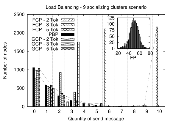
Figure 11: Load balancing for the largest socialized scenario

In order to estimate the benefit of GCP in term of load balancing, we have collected for each simulation (scenarios and algorithms), the number of sent software messages by node. As each simulation have the same network load behaviour, Figure 11 presents the results for the 9 socializing clusters scenario. For each number of message sent (represents by the X-axes), we have represent for all simulations the number of nodes which have sent exactly this number of time its software. As the flooding consumes much more message than the three other algorithms (PBP, FCP and GCP), the network load with flooding is represent in the upper-right corner of Figure 11.

For each scenario, the benefit of GCP or FCP compared to the flooding algorithm is clear. When considering the number of software binary sent, the two other algorithms save between 82 % and 93 % of messages for FCP and more than 98 % for GCP for a 50 seconds simulation only. As we have presented above, the number of software sent message increase according linearly to time with the flooding algorithm.

By focusing only on the three other algorithms, main plots of Figure 11 show the benefits of GCP according to PBP and FCP. In fact, as FCP is not aware of the remote node’s version, the local node sends its own version as long as it still possesses tokens. That implies the number of software sending messages with FCP algorithm is almost constant, corresponding of two times the number of tokens owns by each node ($k$ tokens for the first version plus $k$ tokens for the newer version: in these simulations, the software is updated only once).

With GCP and PBP, the current local version number is sent in the beacon message (Piggy-backing mechanism). So, nodes will not send the first version. They only send the newest version, and only if the beacon sender does not owned the latest version. The total number of software send messages in the network is almost equivalent to the number of participating nodes. Moreover, as every node in the transmission range of a sending node receive the sending version, freely for the sender, the network load benefits using GCP is decrease all the more. Comparing GCP with 5 tokens a node and PBP, which have the same propagation speed, we observe that near 5 % of the nodes have send the software more that 5 times, contrary to GCP where nodes have consumed at most 5 tokens.

We do not represent the load extracted from simulation on the realistic trace because it shares the same aspect as the synthetic ones.

5 Related works

This section presents various works in two related axes namely: data dissemination (or broadcasting) and software update (or reprogramming / code propagation). Among those, we focus on the approaches relying on gossip-based algorithms.

5.1 Dissemination in WSN

Reliable data dissemination shares some goals and assumptions with code propagation. Reliable broadcasting consist in a one-to-all message dissemination (one entry point in the system sends some information to all participating nodes in the network).

Vollset and al. [18] propose a classification of reliable broadcast in two classes: deterministic and probabilistic protocols. Deterministic protocols attempt to enforce hard reliability guarantees, as probabilistic protocols provide guaranteed delivery with a certain probability. This paper concludes that deterministic approach tends to have bad tradeoffs necessary between reliability and scalability/mobility, instead of probabilistic protocols, which do not provide deterministic delivery guarantees. Due to the constraints present in Section 1, we focus on probabilistic protocols to obtain a reliable efficiency in scalability and mobility models.

Some study used geographical information to increase broadcast efficiency (load balancing, propagation speed, …). In [17], several degrees of local information has introduced in broadcast protocols. Subramanian and al. present three degrees of knowledge: no geographic or state information, coarse geographic information about the origin of the broadcast and no geographic information, but remember previously received messages. Authors conclude that local information have a not negligible role in broadcasting in WSN. As our contribution, several works tends to increase the broadcast efficiency without using locality. [8, 14, 15]

Another probabilistic broadcast is based on the gossip-based model [12, 19]. Gossip-based protocol is a promising model for WSN as presented in Section 1. Gossip as a general technique has been used to solve several problems (data management, failure detection, …). In the end of this subsection, we present different gossip-based dissemination protocols for WSNs.

In [12], a reliable broadcast service based on the gossip model is presented. Using probabilistic forwarding, gossip is used to self-adapt the probability of information send for any topology. But, in most case, mobility is not taken into account.

Wang and al. [19] proposed a reliable broadcast protocol for mobile wireless sensor network. By using clustering technique and gossiping, this protocol has high delivery ratio and low end-to-end delay. Another noteworthy work is a reliable multicast protocol for mobile ad-hoc network (MANET), called Anonymous gossip [4]. Based on reliable gossip-based multicast for wired networks, gossip is used to obtain some information about message which node has not yet received. In these two last references, authors are studying MANETs, which have more resources than sensor nodes.

Our works is a transversal axis of these last studies. We are taking into account mobility and power consumption of WSN by using gossip-based paradigm.

5.2 Code propagation in WSN

Recently, gossip-based model has been used in code propagation service [13, 20]. Trickle [13] is a code propagation algorithm using a ”polite gossip” policy. This algorithm permits to propagate and maintain code updates in WSN. It regulates the transmission by gossiping code meta-data. If the information is up-to-date, the receivers stay quiet. Otherwise, if the information is issued from an older version, the gossiper can be brought up to date, and similarly.

Other works propose several protocols to apply code propagation. Deluge [7] assure to reprogramming the network by a reliable data dissemination protocol. Authors argue that Deluge can characterize its overall performance. Notably, they assume that it may be difficult to significantly improve the transmission rate obtained by Deluge. Kulkarni and Wang proposed MNP [11], a multi-hop reprogramming service, by splitting code into several segments. Using pipelining and sleep cycle, this algorithm also guarantees that, in a neighbourhood, there is at most one source transmitting the program at a time. Recently, these authors present Gappa [20], an extension of MNP. Using an Unmanned Ariel Vehicle (UAV), this algorithm can communicate parts of the code to a subset of sensor nodes on a multiple channel at once. The protocol ensures that at any time, there is at most one sensor transmitting on a given frequency.

In the best of our knowledge, none of work treats about code propagation in mobile WSN.

6 Conclusion

In this paper, we have proposed a software update algorithm for mobile wireless sensor networks. As the best of our knowledge, tackle code propagation in mobile WSN has not been done before. Based on leverage works on epidemic protocols and on similarities and differences between P2P systems and mobile WSNs, Gossip-based Code Propagation algorithm tends to outperforms classical dissemination algorithms, with only a small overhead by adding little extra information on sensor nodes and in beacon messages.

We have exposed the benefit of GCP on several simulation scenarios, compared as three other dissemination algorithms: one ideal in speed convergence but with a large number of software send messages and, therefore, very high power consumption, another one based on forwarding control and a last one based on piggy-backing message.

For each of these algorithms, GCP obtains an important profit accordingly to the little overhead information. With a clearly load balance through the network, GCP can disseminate the new software with almost the same propagation speed than the ideal one.

One of these work perspectives consists to include the Delay Tolerant Networks (DTN) paradigm into GCP in order to take into account and optimize the free receptions of the software due to the omnidirectionnal wireless transmission.

References

- [1] I. F. Akyildiz, W. Su, Y. Sankarasubramaniam, and E. Cayirci. A survey on sensor networks. IEEE Communications Magazine, 40(8):102–114, 2002.
- [2] S. Brown and C. J. Sreenan. A new model for updating software in wireless sensor networks. IEEE Network, pages 42–47, November/December 2006.
- [3] M. Castro, P. Druschel, Y. C. Hu, and A. Rowstron. Proximity neighbor selection in tree-based structured peer-to-peer overlays. Technical Report MSR-TR-2003-52, Microsoft Reasearch, Cambridge, UK, 2003.
- [4] R. Chandra, V. Ramasubramanian, and K. Birman. Anonymous gossip: Improving multicast reliability in ad-hoc networks. In International Conference on Distributed Computing Systems (ICDCS 2001), Phoenix, Arizona, April 2001.
- [5] K. Chen and Y. Jian. Survey on peer to peer data dissemination in manet. Computer Information Science Engineering Department, November 2005.
- [6] N. Eagle and A. S. Pentland. CRAWDAD data set mit/reality (v. 2005-07-01). Downloaded from http://crawdad.cs.dartmouth.edu/mit/reality, July 2005.
- [7] J. W. Hui and D. Culler. The dynamic behavior of a data dissemination protocol for network programming at scale. In Proceedings of the 2nd international conference on Embedded networked sensor systems (SenSys’04), pages 81–94, New York, NY, USA, 2004. ACM Press.
- [8] C. Intanagonwiwat, R. Govindan, D. Estrin, J. Heidemann, and F. Silva. Directed diffusion for wireless sensor networking. IEEE/ACM Transactions Networks, 11(1):2–16, February 2003.
- [9] D. B. Johnson and D. A. Maltz. Dynamic source routing in ad hoc wireless networks. Mobile Computing, 353:153–181, 1996.
- [10] A.-M. Kermarrec, L. Massoulié, and A. J. Ganesh. Probabilistic reliable dissemination in large-scale systems. IEEE Transactions on Parallel and Distributed Systems, 14(3), March 2003.
- [11] S. S. Kulkarni and L. Wang. Mnp: multihop network reprogramming service for sensor networks. In the 25th International Conference on Distributed Computing System (ICDCS’05), pages 7–16, Columbus, OH, USA, June 2005.
- [12] P. Kyasanur, R. R. Choudhury, and I. Gupta. Smart gossip: An adaptive gossip-based broadcasting service for sensor networks. In The Third IEEE International Conference on Mobile Ad-hoc and Sensor Systems (MASS 2006), Vancouver, Canada, October 2006.
- [13] P. Levis, N. Patel, S. Shenker, and D. Culler. Trickle: A self-regulating algorithm for code propagation and maintenance in wireless sensor networks. In First Symposium on Network Systems Design and Implementation (NSDI), march 2004.
- [14] N. Li and J. C. Hou. Blmst: A scalable, power-efficient broadcast algorithm for wireless networks. In QSHINE ’04: Proceedings of the First International Conference on Quality of Service in Heterogeneous Wired/Wireless Networks (QSHINE’04), pages 44–51, Washington, DC, USA, 2004. IEEE Computer Society.
- [15] N. Mitton, A. Busson, and E. Fleury. Broadcasting in self-organizing wireless multi-hop network. Research report RR-5487, INRIA, February 2005.
- [16] P. Rentala, R. Musunuri, S. Gandham, and U. Saxena. Survey on sensor networks. In Proceedings of International Conference on Mobile Computing and Networking, 2001.
- [17] S. Subramanian, S. Shakkottai, and A. Arapostathis. Broadcasting in sensor networks: The role of local information. In IEEE, editor, IEEE Infocom, 2006.
- [18] E. Vollset and P. Ezhilchelvan. A survey of reliable broadcast protocols for mobile ad-hoc networks. Technical Report CS-TR-792, University of Newcastle upon Tyne, 2003.
- [19] G. Wang, D. Lu, W. Jia, and J. Cao. Reliable gossip-based broadcast protocol in mobile ad hoc networks. In Mobile Ad-hoc and Sensor Networks: First International Conference, MSN 2005, pages 207–218, Wuhan, China, December 2005.
- [20] L. Wang and S. S. Kulkarni. Gappa: Gossip based multi-channel reprogramming for sensor networks. In Second IEEE International Conference in Distributed Computing in Sensor Systems (DCOSS 2006), pages 119–134, 2006.
- [21] B. Xu and O. Wolfson. Data management in mobile peer-to-peer networks. In S. V. L. N. in Computer Science, editor, Proc. of the 2nd International Workshop on Databases, Information Systems, and Peer-to-Peer Computing (DBISP2P’04), pages 1–15, Toronto, Canada, August 2004.