Spin projected unrestricted Hartree–Fock ground states for harmonic quantum dots.

Abstract

We report results for the ground state energies and wave functions obtained by projecting spatially unrestricted Hartree Fock states to eigenstates of the total spin and the angular momentum for harmonic quantum dots with $N\leq 12$ interacting electrons including a magnetic field. The ground states with the correct spatial and spin symmetries have lower energies than those obtained by the unrestricted method. The chemical potential as a function of a perpendicular magnetic field is obtained. Signature of an intrinsic spin blockade effect is found.

I Introduction

Systems like atoms, metal clusters, trapped bosons and quantum dots show several universal features. reimann For example, strongly interacting electrons in quantum dots arrange themselves in a rotating Wigner molecule. reimann Rotating boson molecules have been predicted to exist in ion traps. RBM Furthermore, symmetric potentials can induce a shell structure in atoms, bohrmottelson metal clusters, clusterrmp and quantum dots. kouwenhoven ; reimann In the latter, signatures of shell structure have been experimentally probed, tarucha ; taruchasci leading to Hund’s rules for the total spin of the electron ground state. The spin in quantum dots kouwenrev also affects the electron transport. It can lead to spin blockade effects weinmann ; weinmann2 and negative differential conductance in nonlinear transport, weinmann ; cavaprlb ; RHCSK2006 ; ciorgaapl ; datta and it induces periodic modulations of the positions of the Coulomb peaks in the linear conductance as a function of an applied magnetic field. roggesb ; hawrylak3 ; hawrylak4 ; RHCSK2006 More recently, the effect of the spatial distribution of the spins on the Kondo phenomenon has been probed. kondorog ; roggekondo ; kondokou ; kondokel

Electron and spin states of quantum dots have been theoretically studied with various techniques. reimann For small electron numbers $N$, exact diagonalization (ED), dineykhan ; pfannkuche ; merkt ; mikhailov2 ; mikhailov ; haw1 ; haw2 ; wojs ; szafran ; maksymB ; kyriakidis ; nishi configuration interaction (CI), wensauer ; rontani and stochastic variational methods varga allow for determining ground and excited state energies and their quantum numbers with high accuracy. For larger $N$, the size of the many-body basis set increases exponentially. With presently available computational technology, reliably converged “exact” results can be obtained only for electron numbers up to $N\approx 8$ electrons. rontani

For $N\leq 13,N=16,24,48$, Quantum Monte Carlo (QMC) pederiva ; egger ; harju ; bolton ; ghosalnp ; ghosal ; pederiva2 ; esa methods have been used. They can provide accurate estimates for ground and excited states energies. With these techniques, the shell structure, Hund’s rules, Wigner crystallization and the occurrence of “magic” angular momenta have been investigated. mikhailov ; harju ; maksym ; ruan ; filinov ; bao ; ghosalnp ; ghosal Most of the results for higher particle numbers have been restricted to zero magnetic field. It is believed that QMC provides better estimates for the energies of the ground states for larger electron numbers as compared to the “exact” methods.

For larger $N$ and/or in the presence of magnetic field $B$, methods like Hartree Fock (HF)  landmanprl ; landman3 ; reusch0 ; reusch ; lipparini ; hawrylak1 ; hawrylak2 and the density functional theory manninen ; hirose ; gattobigio ; harju2 ; esa1 ; esa2 ; esa3 have been used. Generally, these seem to provide less accurate estimates for the ground states which also can have unphysical broken symmetries due to incomplete ansatz wave functions. For instance, neglecting correlations, the straightforward HF method starts from a single Slater determinant as a variational many-body wave function which not necessarily is an eigenstate of the total spin. szabo Spatially unrestricted HF methods (UHF)landmanprl ; reusch0 systematically use symmetry breaking in order to obtain better estimates for the ground state energy. This may lead to wrong results for the total angular momentum and the total spin. For instance, UHF calculations sometimes seem to fail predicting the total spin resulting from Hund’s rule, in contradiction to the more accurate methods. Violations of Hund’s rules for relatively weak Coulomb interactions have been reported landmanprl for $N=4,8,9$.

Projection techniques, pioneered in the 60th of the last century, loewdin1 ; ring ; loewdin2 can be applied for introducing the correct spatial symmetries. In quantum dots, they have been used for obtaining wave functions corresponding to specific angular momenta. landman2 ; landman4 ; landman5 ; koonin ; YL2002 Recently, the random phase approximation has been used to restore the rotational symmetry of wave functions obtained by UHF. serrarpa

Restoring the spin symmetry has received much less attention, and has been used only for very few (up to $N=3$) electrons. landman2 For $N=2$, the spin singlet symmetry has been approximately restored with the Lipkin-Nogami approach. serrarpa Larger $N$ have seldom been treated with the projection technique. degio In view of the recent discussion of spin effects in the transport spectra of quantum dots, information about the total spin is, however, necessary. Additionally, by restoring the symmetries correlations are introduced into the ground state wave function that are absent in a single UHF Slater determinant. This leads to a better estimate for the ground state energy.

In this paper, we apply a projection technique to the states obtained by UHF for estimating the ground state energy of a circular quantum dot with $N\leq 12$ electrons, including a magnetic field. Starting from an UHF Slater determinant with broken rotational symmetry, a first estimate for the ground state energy and the wavefunction is obtained. Then, both the total spin and the angular momentum of the UHF variational wave function are introduced by projecting on the corresponding subspaces. We show that, after restoring all of the symmetries, the energies and the wave functions are improved and show physical features which are not included in the UHF method.

We discuss the efficiency of the projected HF method (PHF) by comparing our results with those of ED, CI, and QMC. We determine the ground state energies as a function of a magnetic field, and obtain the chemical potential that can be measured in transport experiments. Our main findings are:

(i) By projecting the UHF wave functions on the total angular momentum $L$ and on the total spin $S$, the ground state energy is successively lowered. The correction due to the spin projection is generally smaller than the one associated with the angular momentum, but still necessary for determining the correct ground state and its quantum numbers.

(ii) The quantum numbers $L$ and $S$ are correctly reproduced, if the strength of the interaction is not too large. Especially, for $B=0$, the first Hund’s rule — namely that $S$ is maximized for open shells — is recovered for $N\leq 12$ electrons, except for $N=10$, discussed below. Hund’s rule has been claimed earlier to be violated on the basis of UHF results landmanprl .

(iii) By comparing the results with CI and QMC, we estimate a correlation energy, defined as the difference between PHF and “exact” energies, of about 2% of the ground state energy.

(iv) With increasing interaction strength the correlation energy decreases. Nevertheless, for stronger interaction, and larger $N$, the PHF ground state tends to be spin polarized in contrast to more exact results. This is consistent with earlier conjectures, namely that UHF tends to overestimate the influence of the exchange. reusch0

(v) As a function of $B$, several crossovers between ground states with different total spins and angular momenta are found that are absent in UHF. These are associated with characteristic changes in the electron densities. The onset of the singlet–triplet transition hawrylak1 occurring for dot filling factor $\nu\approx 2$ and $N$ even is recovered. Features that lead to an intrinsic spin blockade are predicted.

In the next Section, details of the UHF method are outlined. The consequences of the broken symmetries are described and the projection technique is discussed, with special emphasis on the total electron spin. In Sect. III results for zero and non-zero magnetic field are presented and discussed.

II Model and method

II.1 The model

Consider $N$ electrons in a two-dimensional (2D) quantum dot confined by an in–plane harmonic potential and subject to a perpendicular magnetic field ${\bf B}=B{\bf e}_{z}$. The Hamiltonian is ($\hbar=c=1$)

$${H}=\sum_{i=1}^{N}{h}_{0}({\bf r}_{i},s_{zi})+\frac{1}{2}\sum_{\begin{subarray}{c}i,j=1\\ i\neq j\end{subarray}}^{N}{v}({\bf r}_{i}-{\bf r}_{j})$$ (1)

with

$${h}_{0}({\bf r},s_{z})=\frac{{\left[{\bf p}+e{\bf A}({\bf r})\right]}^{2}}{2m^{*}}+\frac{m^{*}\omega_{0}^{2}}{2}{\bf r}^{2}+g^{*}\mu_{B}Bs_{z}$$ (2)

${\bf r}\equiv(r,\vartheta)$ the 2D polar coordinates, $v({\bf r})={e^{2}}/{4\pi\varepsilon_{0}\varepsilon_{r}r}$ the Coulomb interaction potential, ${\bf B}={\rm rot}{\bf A}$, $m^{*}$ effective electron mass, $\omega_{0}$ confinement frequency, $g^{*}$ effective $g$-factor and $\mu_{B}$ the Bohr magneton. The $z$-component of the $i$-th spin is $s_{zi}=\pm 1/2$, $-e$ the electron charge and $\varepsilon_{0}$ ($\varepsilon_{r}$) the vacuum (relative) dielectric constant. The single-particle term in (1) yields the Fock–Darwin fd (FD) spectrum

$$\epsilon_{n,l,s_{z}}=\Omega\left(2n+|l|+1\right)+\frac{\omega_{c}}{2}l+g^{*}\mu_{B}Bs_{z}\,,$$ (3)

with eigenfunctions $\phi_{n,l}({\bf r})\chi^{\pm}$, where $\chi^{+}$ ($\chi^{-}$) is the spinor corresponding to $s_{z}=+1/2$ ($s_{z}=-1/2$) and fd

$$\phi_{n,l}({\bf r}) = \frac{e^{il\vartheta}}{\ell_{0}}\sqrt{\frac{n!}{\pi(n+|l|)!}}\cdot$$ (4)

$$\cdot\left(\frac{r}{\ell_{0}}\right)^{|l|}e^{-\frac{r^{2}}{2\ell_{0}^{2}}}\mathscr{L}^{|l|}_{n}\left(\frac{r^{2}}{\ell_{0}^{2}}\right)\,.$$

Here, $n$ and $l$ are principal and angular momentum quantum numbers, $\ell_{0}=(m^{*}\Omega)^{-\frac{1}{2}}$ the characteristic oscillator length and $\mathscr{L}_{n}^{|l|}(x)$ the generalized Laguerre polynomial. The cyclotron frequency $\omega_{c}=eB/m^{*}$, and the effective confinement frequency $\Omega=(\omega_{0}^{2}+\omega_{c}^{2}/4)^{1/2}$ are introduced.

At $B=0$, expressing energies in units $\omega_{0}$ and lengths in units $\ell_{0}$, the Hamiltonian (1) depends only on the dimensionless parameter

$$\lambda=\frac{e^{2}}{4\pi\varepsilon_{0}\varepsilon_{r}\ell_{0}\omega_{0}}\,,$$ (5)

which represents the relative strength of the interaction.

II.2 The unrestricted Hartree-Fock method

In HF the Schrödinger equation for a given value of total $S_{z}=s_{z1}+\ldots+s_{zN}$ is solved by using orbitals

$$\psi_{i}^{\alpha}({\bf r})=u_{i}^{\alpha}({\bf r})\chi^{\alpha}\,,\quad\quad\quad 1\leq i\leq N_{\alpha}$$ (6)

with $\alpha=+$ ($\alpha=-$) denoting spin up (down) and $N_{\alpha}$ is the number of electrons with spin $\alpha\cdot 1/2$. They are obtained as the solutions of the coupled integro–differential equations

$$\left[h_{0}({\bf r},\alpha 1/2)+\int{\rm d}{\bf r}^{\prime}\rho({\bf r}^{\prime})v({\bf r}-{\bf r}^{\prime})\right]\psi_{i}^{\alpha}({\bf r})-\sum_{j=1}^{N_{\alpha}}\left[\int{\rm d}{\bf r}^{\prime}\psi_{j}^{\alpha*}({\bf r}^{\prime})\psi_{i}^{\alpha}({\bf r}^{\prime}){v}({\bf r}-{\bf r}^{\prime})\right]\psi_{j}^{\alpha}({\bf r})=\varepsilon_{i}^{\alpha}\psi_{i}^{\alpha}({\bf r})\,,$$ (7)

where $\rho({\bf r})=\rho^{+}({\bf r})+\rho^{-}({\bf r})$ is the HF density

$$\rho^{\alpha}({\bf r})=\sum_{i=1}^{N_{\alpha}}\left|\psi_{i}^{\alpha}({\bf r})\right|^{2}\,.$$ (8)

For a given $S_{z}$, an initial guess for the orbitals $\psi_{i}^{\alpha}({\bf r})$ with $i\leq N_{\alpha}$ is made. Then, HF densities are evaluated and Eqs. (7) are solved to obtain updated orbitals. This is iterated until self-consistency is achieved. The many body wave function is a single Slater determinant, eigenfunction of $S_{z}$,

$$\left|\Psi^{S_{z}}\right> = \frac{1}{\sqrt{N!}}{\rm det}\{\psi_{1}^{+}({\bf r}_{j}),\ldots,\psi_{N_{+}}^{+}({\bf r}_{j})\,,$$ (9)

$$\qquad\qquad\psi_{1}^{-}({\bf r}_{j}),\ldots,\psi_{N_{-}}^{-}({\bf r}_{j})\}\,,$$

that corresponds to a stationary point of the UHF energy szabo ; ring

$$E^{S_{z}}=\frac{\left<\Psi^{S_{z}}\right|H\left|\Psi^{S_{z}}\right>}{\left<\Psi^{S_{z}}\right|\left.\Psi^{S_{z}}\right>}\,.$$ (10)

In order to numerically solve (7) we expand the orbitals in the FD basis $\phi_{\mu}({\bf r})\chi^{\alpha}$ (Eq. (4))

$$\psi_{i}^{\alpha}({\bf r})=\sum_{\mu=1}^{K}C_{\mu i}^{\alpha}\phi_{\mu}({\bf r})\chi^{\alpha}\,,\quad\quad\quad 1\leq\mu\leq K$$ (11)

where $C_{\mu i}^{\alpha}$ are complex coefficients. The truncation of the basis to $K$ states is necessary in order to numerically implement the procedure. We have used the $K=75$ lowest FD states for each value of $B$. This led to fair convergence (see Sec. II.5). Introducing the density matrices

$$P_{\mu\nu}^{\alpha}=\sum_{i=1}^{N_{\alpha}}C_{\mu i}^{\alpha}(C_{\nu i}^{\alpha})^{*}\,,$$ (12)

connected to (8) by

$$\rho^{\alpha}({\bf r})=\sum_{\mu,\nu=1}^{K}\phi_{\mu}({\bf r})P_{\mu\nu}^{\alpha}\phi_{\nu}^{*}({\bf r})\,,$$

it is possible to show that equation (7) is equivalent to the coupled nonlinear Pople–Nesbet eigenvalue problem

$$\sum_{\nu=1}^{K}F_{\mu\nu}^{\alpha}C_{\nu i}^{\alpha}=\varepsilon_{i}^{\alpha}C_{\mu i}^{\alpha}\,.$$ (13)

Here $F_{\mu\nu}^{\alpha}$ are the Fock matrices,

$$F_{\mu\nu}^{\alpha} = \epsilon_{n_{\mu},l_{\mu},\alpha{1}/{2}}\ \delta_{\mu\nu}$$

$$\!\!\!\!\!\!\!\!\!\!\!\!\!\!\!\!\!\!\!\!+\sum_{\lambda,\eta=1}^{K}P_{\lambda\eta}^{\alpha}\left[\langle\mu\eta|v|\nu\lambda\rangle-\langle\mu\eta|v|\lambda\nu\rangle\right]+P_{\lambda\eta}^{-\alpha}\langle\mu\eta|v|\nu\lambda\rangle\,,$$

and the two-body interaction matrix elements

$$\!\!\!\!\!\!\langle\mu\eta|v|\nu\lambda\rangle=$$

$$\!\!\!\!\!\!\int{\rm d}{\bf r}_{1}{\rm d}{\bf r}_{2}\phi_{\mu}^{*}({\bf r}_{1})\phi_{\eta}^{*}({\bf r}_{2})v({\bf r}_{1}-{\bf r}_{2})\phi_{\nu}({\bf r}_{1})\phi_{\lambda}({\bf r}_{2})$$ (15)

can be evaluated analytically. rontani The energy (10) is then

$$E^{S_{z}}=\frac{1}{2}\sum_{\alpha=\pm}\sum_{\mu,\nu=1}^{K}\left[\epsilon_{n_{\nu},l_{\nu},\alpha{1}/{2}}\ \delta_{\nu\mu}+F_{\nu\mu}^{\alpha}\right]P_{\mu\nu}^{\alpha}\,.$$ (16)

We use spatially unrestricted initial conditions landmanprl ; landman2 ; reusch0 with a random distribution of initial $C^{\alpha}_{\mu,\nu}$. This implies initial orbitals without circular symmetry, and leads to better energy estimates. However, symmetry broken Slater determinants are in general neither eigenfunctions of the total angular momentum $L={l}_{1}+\ldots+{l}_{N}$ nor of ${\bf S}^{2}$ (total spin ${\bf S}={\bf s}_{1}+\ldots+{\bf s}_{N}$). szabo

The most general UHF solution is a linear superposition of eigenfunctions $|\Psi^{S_{z}}(L,S)\rangle$ of $L$ and ${\bf S}$

$$|\Psi^{S_{z}}\rangle=\sum_{L=-\infty}^{\infty}\sum_{S\geq|S_{z}|}^{N/2}|\Psi^{S_{z}}(L,S)\rangle\,.$$ (17)

For given $N$ and $S_{z}$, many initial conditions are used. Correspondingly, several stationary points are found. They form a sequence $|\Psi_{k}^{S_{z}}\rangle$ ($k=1,2,\ldots$) with energies $E_{1}^{S_{z}}<E_{2}^{S_{z}}<\ldots$. For a given $S_{z}$, the process is iterated until the lowest $E_{1}^{S_{z}}$ is found. The UHF ground state is defined as,

$$E_{{\rm UHF}}=\mathop{{\rm min}}_{S_{z}}\ \left\{E_{1}^{S_{z}}\right\}\,.$$

II.3 Spin and angular momentum projection

In order to obtain states with specific $L$ and $S$ we act on the UHF Slater determinant with operators ring $\hat{P}_{L}$ and $\hat{P}_{S}^{S_{z}}$ which project on $\hat{L}$ and $\hat{{\bf S}}$, respectively. They satisfy commutation rules $[\hat{P}_{S}^{S_{z}},\hat{P}_{L}]=[\hat{P}_{S}^{S_{z}},\hat{H}]=[\hat{P}_{L},\hat{H}]=0$. Their simultaneous action yields an eigenfunction of $\hat{L}$ and $\hat{{\bf S}}^{2}$, $\hat{P}_{L}\hat{P}^{S_{z}}_{S}|\Psi^{S_{z}}\rangle=|\Psi^{S_{z}}(L,S)\rangle$. The corresponding energy is (Appendix A)

$$E^{S_{z}}(L,S) = \frac{\langle\Psi^{S_{z}}(L,S)|\hat{H}|\Psi^{S_{z}}(L,S)\rangle}{\langle\Psi^{S_{z}}(L,S)|\Psi^{S_{z}}(L,S)\rangle}$$ (18)

$$\equiv \frac{\langle\Psi^{S_{z}}|\hat{H}|\Psi^{S_{z}}(L,S)\rangle}{\langle\Psi^{S_{z}}|\Psi^{S_{z}}(L,S)\rangle}\,.$$

The spin projector

$$\hat{P}_{S}^{S_{z}}=\prod_{k=|S_{z}|,k\neq S}^{N/2}\frac{\hat{S}^{2}-k(k+1)}{S(S+1)-k(k+1)}\ ,$$ (19)

annihilates all the components of (9) with spin different from $S$. loewdin1 Its action is written as loewdin1 ; projS1

$$\hat{P}_{S}^{S_{z}}|\Psi^{S_{z}}\rangle=\sum_{q=0}^{N_{<}}C_{q}(S,S_{z},N)|T_{q}\rangle$$ (20)

where $N_{<}={\rm min}\{N_{+},N_{-}\}$ and

$$C_{q}(S,S_{z},N)=\frac{2S+1}{1+N/2+S}\sum_{k=0}^{S-S_{z}}(-1)^{q+S-S_{z}-k}{S-S_{z}\choose k}{S+S_{z}\choose S-S_{z}-k}{N/2+S\choose S_{z}+N/2-q+k}^{-1}$$ (21)

are the Sanibel coefficients. projS1 ; ruitz The term $|T_{q}\rangle=|T_{q}^{(1)}\rangle+\ldots+|T_{q}^{(n_{q})}\rangle$ is the sum of all

$$n_{q}={N_{+}\choose q}{N_{-}\choose q}$$ (22)

Slater determinants obtained by interchanging, without repetition, all the possible $q$ spinor pairs with opposite spins in $|\Psi^{S_{z}}\rangle$. By definition $\left|T_{0}\right>\equiv|\Psi^{S_{z}}\rangle$.

For example, consider $N=4$, $S_{z}=0$ ($N_{+}=N_{-}=2$),

$$\left|T_{0}\right>=\frac{1}{\sqrt{24}}{\rm det}\{u_{1}^{+}{\chi^{+}},u_{2}^{+}{\chi^{+}},u_{1}^{-}{\chi^{-}},u_{2}^{-}{\chi^{-}}\}\,.$$ (23)

This state is a linear superposition of all spin eigenstates with $S\leq 2$. The spin projection selects a specific spin

$$\hat{P}_{S=0}^{S_{z}=0}\left|\Psi^{S_{z}=0}\right>=\frac{1}{3}|T_{0}\rangle-\frac{1}{6}|T_{1}\rangle+\frac{1}{3}|T_{2}\rangle\,,$$ (24)

$$\hat{P}_{S=1}^{S_{z}=0}\left|\Psi^{S_{z}=0}\right>=\frac{1}{2}|T_{0}\rangle-\frac{1}{2}|T_{2}\rangle\,,$$ (25)

$$\hat{P}_{S=2}^{S_{z}=0}\left|\Psi^{S_{z}=0}\right>=\frac{1}{6}|T_{0}\rangle+\frac{1}{6}|T_{1}\rangle+\frac{1}{6}|T_{2}\rangle\,,$$ (26)

where

$$|T_{1}\rangle = \frac{1}{\sqrt{24}}\left[{\rm det}\{u_{1}^{+}{\chi^{+}},u_{2}^{+}{\chi^{-}},u_{1}^{-}{\chi^{+}},u_{2}^{-}{\chi^{-}}\}\right.+$$

$$+ {\rm det}\{u_{1}^{+}{\chi^{+}},u_{2}^{+}{\chi^{-}},u_{1}^{-}{\chi^{-}},u_{2}^{-}{\chi^{+}}\}+$$

$$+ {\rm det}\{u_{1}^{+}{\chi^{-}},u_{2}^{+}{\chi^{+}},u_{1}^{-}{\chi^{+}},u_{2}^{-}{\chi^{-}}\}+$$

$$+ \left.{\rm det}\{u_{1}^{+}{\chi^{-}},u_{2}^{+}{\chi^{+}},u_{1}^{-}{\chi^{-}},u_{2}^{-}{\chi^{+}}\}\right]\,,$$

$$|T_{2}\rangle = \frac{1}{\sqrt{24}}{\rm det}\{u_{1}^{+}{\chi^{-}},u_{2}^{+}{\chi^{-}},u_{1}^{-}{\chi^{+}},u_{2}^{-}{\chi^{+}}\}\,.$$

Summing up equations (24)—(26) results in the original determinant $|\Psi^{S_{z}}\rangle$, since $\sum_{S}\hat{P}_{S}^{S_{z}}=1$.

The projector on $\hat{L}$ is given by ring

$$\hat{P}_{L}=\frac{1}{2\pi}\int_{0}^{2\pi}{\rm d}\gamma\ e^{-iL\gamma}e^{i\hat{L}\gamma}\,,$$ (27)

where $\exp{(i\hat{L}\gamma)}$ acts on $|T_{q}\rangle$ rotating by $\gamma$ around the $z$ axis all spatial parts of the orbitals

$$u_{i}^{\alpha}(r,\vartheta)\rightarrow u_{i}^{\alpha}(r,\vartheta+\gamma)\,.$$

We denote this by $|T_{q}(\gamma)\rangle$. Using (20) and (27) we get

$$|\Psi^{S_{z}}(L,S)\rangle = \frac{1}{2\pi}\sum_{q=0}^{N_{<}}C_{q}(S,S_{z},N)\cdot$$ (28)

$$\cdot\int_{0}^{2\pi}{\rm d}\gamma\ e^{-iL\gamma}|T_{q}(\gamma)\rangle\,.$$

The projected state (28) is a sum of many Slater determinants (Appendix A). This indicates that correlation has been introduced by the projection.

The main computational effort is due to the evaluation of two-body matrix elements in (18). Projecting an $N$-particle UHF state with $S_{z}$ to a state with total spin $S$ requires to evaluate $n({S_{z}},N)=\sum_{q=0}^{N_{<}}n_{q}$ terms,

$$n(S_{z},N)={N\choose N/2+S_{z}}.$$ (29)

For $N$ even (odd), the worst case is $S_{z}=0$ ($S_{z}=1/2$).

For the angular momentum projection we use a fast Fourier transform (FFT) and partition the integration interval $[0,2\pi]$ in $n(L)$ points; $n(L)$ is determined by the angular momentum range $|L|\leq L_{max}$ for which good convergence (relative error $<10^{-6}$) of the PHF energies is required. We have checked that for $L_{max}=20$ $n(L)=256$ is needed. Using FFT, all energy values for given $S$ and $|L|\leq L_{max}$ are simultaneously available, which considerably accelerates the calculation with respect to performing distinct computations for each value of $L$. The total number of two-body matrix elements is $n_{tot}=n({S_{z}},N)n(L)$.

$N$	$n_{tot}$	$n$
2	512
4	1536	19774szafran
6	5120	661300rontani
8	17920
10	64512
12	236544
14	878592
16	3294720

Table 1: Numbers of two-body matrix elements used for PHF, $n_{tot}$ required to evaluate $E^{S_{z}=0}(L,S)$ for even $N\leq 16$, $S_{z}=0$, $S\leq N/2$, and $|L|\leq 20$ (see text). Last column: some numbers used in other methods.

Table 1 shows $n_{tot}$ for the case of even $N\leq 16$ and $L_{max}=20$ in the worst case $S_{z}=0$. This is the $L_{max}$ value used in the paper. Although $n_{tot}$ quickly increases as a function of $N$, especially because (29) grows exponentially for large $N$, it still compares favorably with respect to exact methods. For example, previously reported ED calculations szafran used a basis of 19774 Slater determinants for $N=4$, $S_{z}=0$, $S=2$, and $L=14$. CI calculations rontani for $N=6$, $S_{z}=0$, $S=0$, $L=0$ need 661300 configurational state functions (linear superposition of Slater determinants).

II.4 Determining the PHF ground state

To determine the ground state, it is generally not sufficient to project only the UHF ground state. If several UHF solutions (Sec. II.2) are almost degenerate, all of the $|\Psi_{i}^{S_{z}}\rangle$ have to be projected. The PHF ground state is then defined by

$$E_{{\rm PHF}}=\mathop{{\rm min}}_{\{i,S_{z},L,S\}}\ \left\{E_{i}^{S_{z}}(L,S)\right\}\,.$$ (30)

One can show that projecting arbitrary UHF Slater determinants on $L$ and $S$ always leads to energies that are not lower than the exact ground state energy, thus satisfying the variational principle.

As an example, we consider $N=4$ for $B=0$, with confinement energy $\omega_{0}=0.741$ meV. We assume the standard GaAs parameters, $m^{*}=0.067\ m_{e}$ and $\varepsilon_{r}=12.4$. The confinement corresponds to $\lambda=4$. For each $S_{z}$, we have used more than 500 UHF initial conditions. We found two solutions with $S_{z}=0$, and one for $S_{z}=1$ and $S_{z}=2$. The corresponding energies $E^{S_{z}}_{i}$ are given in Tab. 2.

$S_{z}$	$E_{i}^{S_{z}}$	$\!\!E_{i}^{S_{z}}(L,S)$	$L$ $S$
0	19.612	19.356	0 0
		19.404	1 1
	19.641	$19.331^{\star}$	0 1
		19.515	2 0
1	19.608	19.342	0 1
		19.394	1 1
2	19.581⋆	19.516	2 2

Table 2: PHF for $N=4$ for a GaAs quantum dot with $B=0$, $\omega_{0}=0.741$ meV, $m^{*}=0.067\ m_{e}$, $\varepsilon_{r}=12.4$, $\lambda=4$; 2nd column: UHF energy $E_{i}^{S_{z}}$ (units $\omega_{0}$); 3rd column: PHF energy $E_{i}^{S_{z}}(L,S)$ (units $\omega_{0}$); 4th column: PHF quantum numbers. Ground states are indicated by ^⋆.

The UHF ground state corresponds to $S_{z}=2$. Applying the projection to each UHF state, we obtain $E_{i}^{S_{z}}(L,S)$ with different quantum numbers $L$ and $S$: the lowest two are given. The PHF ground state corresponds to $L=0$ and $S=1$. The latter is obtained by projecting the energetically higher UHF minimum with $S_{z}=0$.

II.5 Some comments about errors

The major systematic error of the UHF approximation is the neglect of correlations. By projecting the slater determinant on fixed angular momentum and spin PHF attempts to correct for these effects. A second systematic effect is due to the uncertainty if the self consistent HF procedure has converged towards the absolute minimum of the energy.

In determining the UHF ground state energies, we have checked that the convergence with respect to the size of the basis set is better than $10^{-6}$.

For getting insight into the above systematic effects one can start from wave functions with the same $L,S$ but originating from UHF states with different $S_{z}$. They should be degenerated at $B=0$. In the example of Tab. 2, these are the pairs $|\Psi_{1}^{0}(1,1)\rangle$, $|\Psi_{1}^{1}(1,1)\rangle$ and $|\Psi_{2}^{0}(0,1)\rangle$, $|\Psi_{1}^{1}(0,1)\rangle$. Their energetic differences are $0.010\ \omega_{0}$ and $0.011\ \omega_{0}$, respectively. This corresponds to a relative uncertainty of $5\cdot 10^{-4}$. Similar estimates for the “degeneracy error” is obtained from data for different $N$ and $\lambda$. We attribute the degeneracy error mainly to UHF: different UHF states in different $S_{z}$ sectors approximate the true states with different precision. Therefore, their projection on the same $L,S$ sector does not yield exactly degenerate states.

By comparing our results with other works (see below), the PHF ground state energies for $N\geq 3$ remain about 2% higher than those obtained with ED and QMC. This can be attributed to correlations beyond those introduced by the projection. This also is the limiting factor for the ground state quantum numbers in the regime $N\geq 6$ and $\lambda\geq 4$ where too high polarization are obtained.

When several PHF energies $E^{S_{z}}_{i}(L,S)$ are almost degenerate, one can improve further the ground state: linear superposition of the almost degenerate states $|\Psi^{S_{z}}_{i}(L,S)\rangle$ may result in further lowering of the energy. Here, we have not systematically investigated this effect.

III Results

III.1 Zero magnetic field

III.1.1 Ground state energies

$N$	$\lambda$	$E_{\rm PHF}$	$L$ $S$	$E_{\rm CI}$	$E_{\rm DMC}$	$L$ $S$
2	1.89	3.817	0 0		3.649	0 0
	2	3.885	0 0	3.7295		0 0
	4	4.983	0 0	4.8502		0 0
3	1.89	8.154	1 1/2		7.978	1 1/2
	2	8.337	1 1/2	8.1671		1 1/2
	4	11.131	0 3/2	11.043		1 1/2
4	1.89	13.554	0 1		13.266	0 1
	2	13.899	0 1	13.626		0 1
	4	19.330	0 1	19.035		0 1
5	1.89	20.264	1 1/2		19.764	1 1/2
	2	20.811	1 1/2	20.33		1 1/2
	4	29.501	1 1/2	28.94		1 1/2
6	1.89	27.905	0 0		27.143	0 0
	2	28.703	0 0	27.98		0 0
	4	41.187	0 3	40.45		0 0
7	1.89	36.627	2 1/2		35.836	2 1/2
	2	37.698	2 1/2
	4	54.497	0 5/2	(54.68)	53.726	(2)2 (1/2)1/2
8	1.89	46.260	0 1		45.321	0 1
	2	47.659	0 1	47.14	46.679	0 1
	4	69.479	0 4	70.48		0 1
9	1.89	56.853	0 3/2		55.643	0 3/2
10	1.89	68.245	0 0		66.8785	2 1
		(68.283)	2 1		(66.8789)	0 0
11	1.89	80.444	0 1/2		78.835	0 1/2
12	1.89	93.661	0 0		91.556	0 0

Table 3: Ground state energies from PHF for $N\leq 12$ and $\lambda=1.89$, $2$, $4$ with corresponding $L$, $S$ ($m^{*}=0.067\ m_{e}$, and $\varepsilon_{r}=12.4$) together with results from CI rontani , and DMC (Ref. pederiva, for $\lambda=1.89$, Ref. ghosal, for $\lambda\geq 2$). All energies are in units $\omega_{0}$.

Table 3 summarizes our results for the ground state energies at $B=0$, for $N\leq 12$ and $\lambda=1.89$, $2$, $4$. Results obtained with Diffusion Monte Carlo (DMC) pederiva ; ghosal and CI rontani are included.

For $\lambda\leq 2$, angular momenta and total spins of the ground states obtained by PHF agree with DMC and CI. The total spin fulfills Hund’s first rule: a singlet state for the filled shells ($N=2,6,12$), a triplet for $N=4,8$ and $S=3/2$ for $N=9$. Only for $N=10$, Hund’s rule is not fulfilled since we find $S=0$ instead of $S=1$. However, here the degeneracy error is $0.064\,\omega_{0}$, larger than the energy distance $\Delta E=0.038\,\omega_{0}$ between the ground and the first excited state. Also DMC pederiva predicts an extremely small energy gap between the singlet and the triplet, though it yields an $S=1$ ground state.

Increasing the interaction strength ($\lambda=4$) PHF still produces energies consistent with CI and DMC. However, for $N=3,6,7,8$ incorrect quantum numbers are predicted with a tendency towards polarization. Whenever polarization occurs the ground states have low angular momenta in PHF.

For $\lambda>4$, preliminary results indicate deviations of PHF with respect to CI, DMC. They are reminiscent of the tendency of HF to predict spin polarized ground states due to overestimating the exchange as compared to correlations.

The relative deviation $\delta=(E_{\rm PHF}-E_{\rm DMC})/E_{\rm DMC}$ forpederiva $\lambda=1.89$ and $2\leq N\leq 12$ is shown in Fig. 1; $\delta$ is largest for the closed shells $N=2,6,12$. Except for $N=2$, $\delta\approx 2$%. The inset shows $\delta$ for $N=2$ (squares, with $L,S=0,0$), $N=4$ (dots, with $L,S=0,1$), and $N=6$ (triangles, with $L,S=0,0$) within $1.89\leq\lambda\leq 8$. A decrease with $\lambda$ according to a power law is observed, $\lambda^{-\beta(N)}$. By numerically fitting the data, one finds $\beta(2)=0.57$, $\beta(4)=0.44$ and $\beta(6)=0.45$.

Figure 1: Deviations $\delta$ between PHF and DMC pederiva for $2\leq N\leq 12$, with $\lambda=1.89$ (Tab. 3). Inset: double logarithmic plot of $\delta({\lambda})$ from PHF and QMCpederiva ($\lambda=1.89$), QMC ghosal and CI rontani ($\lambda\geq 2$) for $N=2$ (squares), $N=4$ (dots) $N=6$ (triangles). Lines: best fits to data.

$E_{i}^{S_{z}}$	$S_{z}$	$E_{i}^{S_{z}}(L)$	$L$	$E_{i}^{S_{z}}(L,S)$	$S$	$E_{\rm DMC}$
48.150	0	47.842	0	47.6590	1	46.679
			0	48.0311	2
		48.088	2	47.790${}^{\ }$	0	46.875
			2	47.7994	1
		47.971	1	47.8172	2	46.917
			1	48.0283	1
		48.076	4	47.777${}^{\ }$	0	46.779
48.237	0	47.981	0	47.805${}^{\ }$	0	46.807
		48.025	1	47.9103	1
48.131	1	47.796	2	47.7424	1	46.756
		47.887	1	47.8062	2	46.917
			1	47.9853	1
		48.022	0	47.9771	2	47.406
			0	47.9970	1
48.243	2	47.896	1	47.8812	2
48.335	3	48.129	3	48.126${}^{\ }$	3	47.404

Table 4: Comparison of the lowest energies $E_{i}^{S_{z}}$ obtained from UHF, followed by projection on angular momentum, $E_{i}^{S_{z}}(L)$, and total spin, $E_{i}^{S_{z}}(L,S)$ for $N=8$, $\lambda=2$ ($m^{*}=0.067\ m_{e}$, $\varepsilon_{r}=12.4$). Last column: energies from DMC. ghosal The ground state has $L,S=0,1$. Superscripts ^0,1,2,3,4 denote “degenerated” energies with the same quantum numbers $L,S$ but originating from different $S_{z}$. All energies are in units $\omega_{0}$.

Table 4 and Fig. 2 illustrate the effect of angular momentum projection alone followed by spin projection for $N=8$ starting with UHF states with $S_{z}=0,\ldots,3$. The energy $E_{i}^{S_{z}}(L)$ projected on angular momentum is

$$E_{i}^{S_{z}}(L)=\frac{\langle\Psi_{i}^{S_{z}}|H|\Psi_{i}^{S_{z}}(L)\rangle}{\langle\Psi_{i}^{S_{z}}|\Psi_{i}^{S_{z}}(L)\rangle}\,,$$ (31)

where $|\Psi_{i}^{S_{z}}(L)\rangle=P_{L}|\Psi_{i}^{S_{z}}\rangle$. Only the lowest energies are included in the table.

The typical energy gain obtained by angular momentum projection is about $0.25\,\omega_{0}$. The spin projection induces corrections of the same order of magnitude, which can even change the sequence of energies (Fig. 2).

Figure 2: Influence of the projection procedure on the energy levels (unit $\omega_{0}$) for $N=8$ and $\lambda=2$. Only the two lowest UHF states (left) directly involved in the determination of the PHF ground state (right) are shown.

From the UHF state with $S_{z}=0$ and $E_{1}^{0}=48.150\,\omega_{0}$, which is not the UHF ground state, projection on $L=0$ yields $E_{1}^{0}(L=0)=47.842\,\omega_{0}$. After projection on the total spin we obtain the energy of the ground state, $E_{1}^{0}(L,S=0,1)=47.659\,\omega_{0}$ and an excited state at $E_{1}^{0}(L,S=0,2)=48.031\,\omega_{0}$. On the other hand, the energetically lowest UHF minimum $E_{1}^{1}=48.131\,\omega_{0}$ turns out to yield the first excited PHF state at $E_{1}^{1}(L,S=2,1)=47.742\,\omega_{0}$.

Thus, PHF not only introduces a lowering of the energies but can also restore the correct ordering of energy levels. This can be seen from the last column of Tab. 4, which contains the results obtained by DMC ghosal . Restoring the spin plays a crucial role in obtaining all correct quantum numbers for the ground state including Hund’s rule. degio For example with angular momentum projection alone, one would have predicted $L=2$ for the ground state, in contrast to the correct result.

The degeneracy error for this case is approximately $0.06\ \omega_{0}$ (some example of almost degenerate states are included in Tab. 4). The distance between ground state and the first excited state is $\approx\ 0.08\ \omega_{0}$. This suggests that the ground state for $N=8$ has $L,S=0,1$, consistent with DMC. Even the quantum numbers of the first three excited states turn out to be reproduced correctly while the 4th and the 5th appear to be interchanged.

III.1.2 Ground state densities

For the spin-resolved densities

$$\rho_{{\rm PHF}}^{\alpha}(r)=\frac{\langle\Psi^{S_{z}}(L,S)|\sum_{i=1}^{N_{\alpha}}\delta({\bf r}-{\bf r}_{i})\delta_{s_{zi},\alpha\cdot 1/2}|\Psi^{S_{z}}(L,S)\rangle}{\langle\Psi^{S_{z}}(L,S)|\Psi^{S_{z}}(L,S)\rangle}\,$$

we first consider $N=3$ and $N=4$ (Figs. 3 and 4) for intermediate ($\lambda=2$) and strong ($\lambda=8$) interaction. Increasing the interaction strength leads to a shift of the maximum of the densities towards higher $r$, consistent with earlier findings by ED. mikhailov ; mikhailov1 This is clearly observed in the spin up density for $N=3$ (Fig. 3). For $N=4$, the ground state ($L=0$, $S=1$, $S_{z}=0$) densities $\rho_{{\rm PHF}}^{+}(r)=\rho_{{\rm PHF}}^{-}(r)$ (Fig. 4) agree very well with ED mikhailov for large $r$. Generally, deviations occur near $r\approx 0$.

Figure 3: Spin resolved densities $\rho_{{\rm PHF}}^{\alpha}(r)$ (thick line: $\alpha=+$; thin line: $\alpha=-$) for a GaAs quantum dot with $N=3$, $L=1$, $S=1/2$, and $S_{z}=1/2$ for interaction strengths $\lambda=2$ (solid), $\lambda=8$ (dashed). Density unit: $\pi^{-1}\ell_{0}^{-2}$. Data from ED: mikhailov1 squares $\lambda=2$, circles $\lambda=8$.

Figure 4: Spin resolved densities $\rho_{{\rm PHF}}^{+}(r)=\rho_{{\rm PHF}}^{-}(r)$ for a GaAs quantum dot with $N=4$, $L=1$, $S=1$, and $S_{z}=0$ for $\lambda=2$ (solid line), $\lambda=8$ (dashed line). Density unit: $\pi^{-1}\ell_{0}^{-2}$. Data from ED: mikhailov squares $\lambda=2$, circles $\lambda=8$.

Figure 5(a) shows the total electron density for $N=5$, $L,S=1,1/2$, for $\lambda=0.5,2,10$. For weak interaction, $\lambda=0.5$ (solid line), we find good agreement with CI rontani5 (squares). For $\lambda=2$ (dashed) small deviations near $r=0$ are found.

Figure 5: Densities for $N=5$ $L=1$, $S=1/2$, and $S_{z}=1/2$. (a) Total density $\rho_{{\rm PHF}}(r)=\rho_{{\rm PHF}}^{+}(r)+\rho_{{\rm PHF}}^{-}(r)$ (units $\pi^{-1}\ell_{0}^{-2}$) for $\lambda=0.5$ (solid), $\lambda=2$ (dashed), $\lambda=10$ (dashed-dotted). Squares, circles and triangles: data from CI. rontani5 (b) Spin resolved densities $\rho_{{\rm PHF}}^{\alpha}(r)$ (solid: $\alpha=+$, dashed: $\alpha=-$, units $\pi^{-1}\ell_{0}^{-2}$) for $\lambda=2$. Squares, circles: data from CI. rontani5 (c) Same as (b) but $\lambda=10$.

Figure 5(b) indicates that the spin-down density is responsible for the small deviation from the exact result around $r=0$ for $\lambda=2$.

III.2 Finite magnetic field

In this section, we show results for $N=5,6,7$ in the presence of a magnetic field, $B\leq 2.4\ {\rm T}$, corresponding to a dot filling factor $\nu\gtrsim 2$ ($N\leq 4$ has been discussed in Ref. degio, ). We assume here a confinement $\omega_{0}=6$ meV (corresponding to $\lambda=1.45$) and $g^{*}=-0.44$. For $B>0$, due to the Zeeman term, the PHF ground state always has $S_{z}=S$. Therefore, we do not specify $S_{z}$ in the following.

Figure 6: Ground state energy $E$ (units $\omega_{0}$) as a function of magnetic field $B$ (units T) for $N=5$. Solid: UHF; dashed: angular momentum projection; dashed-dotted: PHF. Here, and in the following figures, $m^{*}=0.067\ m_{e}$, $\varepsilon_{r}=12.4$, $g^{*}=-0.44$, and $\omega_{0}=6$ meV.

We start with $N=5$ (Fig. 6) and $N=6$ (Fig. 7). We show the UHF ground state energy $E_{{\rm UHF}}$ (solid line), the energy obtained from angular momentum projection (dashed, Eq. (31)), and the PHF energy (dashed-dotted, Eq. (30)). The highest energy gain is here due to the angular momentum projection. Spin projection leads to a further decrease of the ground state energy. Obviously, UHF and PHF results behave completely differently with $B$.

For instance, for $N=5$ (Fig. 6) the UHF ground state shows crossovers $S_{z}=1/2\to 3/2$ at $B\approx 0.9\ {\rm T}$ and $S_{z}=3/2\to 1/2$ at $B\approx 1.5\ {\rm T}$. In contrast, the PHF energy has total spin $S=1/2=S_{z}$ in the entire magnetic field region. The state with $S_{z}=3/2$, not compatible with the total spin $S=1/2$, is certainly an artifact of UHF. The crossover $L,S=1,1/2\to L,S=4,1/2$ with increasing magnetic field at $B=1.4\ {\rm T}$ agrees quantitatively with the earlier results obtained by ED. tavernier

Figure 7: Ground state energy $E$ (units $\omega_{0}$) as a function of magnetic field $B$ (units T) for $N=6$. Solid: UHF; dashed: angular momentum projection; dashed-dotted: PHF.

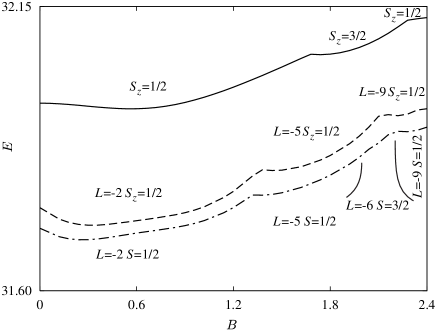
Figure 8: Ground state energy $E$ (units $\omega_{0}$) as a function of magnetic field $B$ (units T) for $N=7$. Solid: UHF; dashed: angular momentum projection; dashed-dotted: PHF.

For $N=6$ (Fig. 7), UHF (solid line) displays no $S_{z}$ transitions. When rotational symmetry is restored, two crossovers, (a) $L=0\to-3$ and (b) $L=-3\to-6$ appear. Performing the spin projection, singlet states corresponding to $L=0$ and $L=-6$ are found, and $S=1$ for $L=-3$ is obtained. Singlets have the largest energy gain, leading to a shift of the features found with angular momentum projection (Fig. 7). Also here, the PHF quantum numbers agree with the earlier results obtained by ED, tavernier including the magnitudes of the crossover fields at $B\approx 1\ {\rm T}$ and $B\approx 1.8\ {\rm T}$ respectively.

The singlet-triplet crossover occurring for $N=6$ at $B\approx 1.8\ {\rm T}$, corresponds to a filling factor $\nu\approx 2$, and is a peculiar feature which is confirmed by several experimental and theoretical studies. hawrylak3 ; hawrylak4 ; hawrylak1 ; tarucha2 Also for $N=8$ preliminary data indicate such a crossover near $\nu=2$. These crossovers are completely absent in UHF (Fig. 7).

Most interesting is $N=7$ (Fig. 8): near $B\approx 2.2\ {\rm T}$ the ground state has $S=3/2$. This can only be obtained including the spin projection and leads eventually to a spin blockade in the transport (see below).

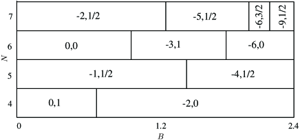
Figure 9: Scheme of the quantum numbers $L,S$ of the PHF ground state as a function of the magnetic field $B$ (units T) for $4\leq N\leq 7$.

In Fig. 9 we show the scheme of the ground state quantum numbers for $4\leq N\leq 7$, as obtained by PHF. They qualitatively agree with previous calculations, maksymB ; tavernier performed for $N\leq 6$. In the region of $B$, where the ground state of $N=7$ has $S=3/2$ the state with $N=6$ is a singlet. Since $\Delta S>1/2$ between the two ground states a spin blockade in the $6\leftrightarrows 7$ transition can be expected near the edge of $\nu=2$ for $N=7$ electrons, for $B\approx 2.3\ {\rm T}$. We note in passing that the lowest excited states for $N=7$, with $L=-5,S=1/2$ and $L=-9,S=1/2$, are at most $\approx 0.07$ meV ($\approx 0.8$ mK) higher in energy. Therefore, it may be difficult to experimentally observe this blockade.

The chemical potential traces $\mu_{N}(B)=E_{{\rm PHF}}(N,B)-E_{{\rm PHF}}(N-1,B)$ obtained by PHF when varying $B$ are experimentally accessible via Coulomb blockade.

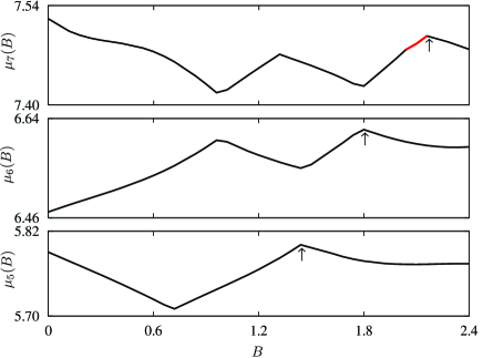
Figure 10: Chemical potentials $\mu_{5}(B)$, $\mu_{6}(B)$, $\mu_{7}(B)$ (units $\omega_{0}$) as a function of $B$ (unit T). Arrows: edge of filling factor $\nu=2$ for $N=5$ (bottom panel), $N=6$ (center), $N=7$ (top). Red line: region of intrinsic spin blockade (see text).

Figure 10 shows $\mu_{5}(B)$, $\mu_{6}(B)$ and $\mu_{7}(B)$. Arrows indicate the onset of $\nu=2$ for the configuration with $N=5$ (bottom panel), $N=6$ (center), $N=7$ (top). The chemical potentials exhibit features related to the above discussed crossovers between ground states. At the onset of $\nu=2$, the chemical potentials exhibit a cusp. For even $N$, this corresponds to the above mentioned singlet-triplet transition. hawrylak1 Generally, the chemical potentials show kinks when quantum numbers of the ground states change (Figs. 9 and 10).

IV Conclusion

We have described a systematic procedure to overcome some of the limitations of UHF approach. Using angular momentum and total spin projections, we have introduced correlations that provide lower estimates for the ground state energies, besides determining the spin and the angular momentum. Several sources of errors have been discussed. In particular, a degeneracy error has been found to be useful for deciding whether or not the estimate for the ground state is plausible.

The procedure yields results consistent with earlier findings for interaction strengths $\lambda\lesssim 2$ which corresponds to experimentally relevant confinement energies $\omega_{0}\gtrsim 3$ meV for $\varepsilon_{r}=12.4$. kouwenhoven ; tarucha

For $B=0$ and $\lambda\leq 2$, we have confirmed Hund’s first rule for the dot total spin, except for $N=10$. In this case, the ground state is ambiguous, since the energy gap between ground and first excited state is smaller than the degeneracy error, consistent with other results. For stronger interaction, $\lambda>4$, deviations from Hund’s rules are obtained, accompanied by the well–known exchange induced tendency of HF–based methods to favor ground states with higher spins and zero angular momenta.

We have shown that PHF predicts correctly the features of the ground state energy as a function of $B$. We have found a spin blockade in the transport between $N=6$ and $N=7$, occurring at a filling factor $\nu\approx 2$.

Given the slower increase in computational effort with particle number described in Sec. II.3 (Tab. 1), as compared to other methods, we hope by parallelization of our code to obtain in the future results for higher number of particles ($N\geq 20$), varying $B$, for interaction strengths relevant to quantum dot experiments, $\lambda\leq 2$.

That the densities are correctly reproduced suggests that tunneling rates between the quantum dot and attached leads needed for electron transport can be reasonably well estimated when using PHF wave functions. This might be useful for providing quantitative results for predicting the heights of the Coulomb blockade peaks as a function of $B$.roggekondo ; hawrylak3 ; RHCSK2006

This work has been supported by the Italian MIUR via PRIN05, by the European Union via MRTN-CT-2003-504574 contract and by the SFB 508 “Quantenmaterialien” of the Universität Hamburg.

Appendix A Some details of the implementation

We provide some technical details about the implementation of the projection technique outlined in Sec. II.3. In order to obtain (18), we have to evaluate the overlaps

$$\langle\Psi^{S_{z}}|\Psi^{S_{z}}(L,S)\rangle=\frac{1}{2\pi}\int_{0}^{2\pi}{\rm d}\gamma\ e^{-iL\gamma}\cdot$$

$$\sum_{q=0}^{N_{<}}\sum_{i=1}^{n_{q}}C_{q}(S,S_{z},N)\langle T_{0}|T_{q}^{(i)}(\gamma)\rangle\,,$$ (32)

and the Hamiltonian matrix elements

$$\langle\Psi^{S_{z}}|H_{0}+V|\Psi^{S_{z}}(L,S)\rangle=\!\frac{1}{2\pi}\int_{0}^{2\pi}{\rm d}\gamma\ e^{-iL\gamma}\cdot$$

$$\sum_{q=0}^{N_{<}}\sum_{i=1}^{n_{q}}C_{q}(S,S_{z},N)\langle T_{0}|H_{0}+V|T_{q}^{(i)}(\gamma)\rangle\,,$$ (33)

with

$$H_{0}+V=\sum_{i=1}^{N}\left[h_{0}({\bf r}_{i},s_{zi})+\frac{1}{2}\sum_{\begin{subarray}{c}j=1\\ j\neq i\end{subarray}}^{N}\!v({\bf r}_{i}-{\bf r}_{j})\!\right]\,.$$ (34)

In the following, we avoid explicit reference to electron coordinates unless when strictly necessary.

Previously, analytic expressions for (18) have been reported landman2 for $N=2$. For larger $N$, however, the number and the complexity of the above matrix elements increases dramatically. This eventually requires numerical treatment.

For evaluating $|T_{q}\rangle=\sum_{i=1}^{n_{q}}|T_{q}^{(i)}\rangle$, we need to generate all the $n_{q}$ swaps of $q$ opposite spin pairs in $|T_{0}\rangle$. The latter correspond to a special class of permutations, acting on the $k$-th component of the generalized vector

$${\bm{\sigma}}=\left(\chi^{+},\ldots,\chi^{+},\chi^{-},\ldots,\chi^{-}\right)$$ (35)

with the correspondence $k\to\pi_{k}^{(q,i)}$. One then has

$$|T_{q}\rangle=\frac{1}{\sqrt{N!}}\sum_{i=1}^{n_{q}}{\rm det}\{w_{1}\sigma_{\pi^{(q,i)}_{1}},\dots,w_{N}\sigma_{\pi^{(q,i)}_{N}}\}\,,$$ (36)

with

$${\bm{w}}=\left(u_{1}^{+},\ldots,u_{N_{+}}^{+},u_{1}^{-},\ldots,u_{N_{-}}^{-}\right)\,.\\$$ (37)

All the permutations are pre-tabulated at the beginning of the calculation. Further calculations are performed by means of well known theorems loewdin2 for many body wave functions. The overlap term is

$$\langle T_{0}|T_{q}^{(i)}(\gamma)\rangle={\rm det}\{d^{(q,i)}(\gamma)\}$$ (38)

where $d^{(q,i)}$ is the overlap matrix

$$d^{(q,i)}_{kp}(\gamma)=\langle w_{k}|w_{p}(\gamma)\rangle\langle\sigma_{k}|\sigma_{\pi^{(q,i)}_{p}}\rangle\,.$$ (39)

Here, $1\leq k,p\leq N$ and $w_{p}(\gamma)$ is a shorthand notation for the rotated spatial part $w_{p}(r,\vartheta+\gamma)$. The term $\langle\sigma_{k}|\sigma_{\pi^{(q,i)}_{p}}\rangle$ reduces to a Kronecker delta. For the evaluation of $\langle w_{k}|w_{p}(\gamma)\rangle$ we use the FD basis, which is particularly convenient to describe rotations. The spatial parts transform as

$$w_{p}(r,\theta+\gamma)=\sum_{\mu=1}^{K}C_{\mu i}^{\alpha_{p}}e^{il_{\mu}\gamma}\phi_{\mu}(r,\theta)$$ (40)

with $l_{\mu}$ the angular momentum of the $\mu$–th FD state, $\alpha_{p}=+$ for $p\leq N_{+}$ and $\alpha_{p}=-$ for $N_{+}+1\leq p\leq N$. Therefore,

$$\langle w_{k}|w_{p}(\gamma)\rangle=\sum_{\mu=1}^{K}(C_{\mu k}^{\alpha_{k}})^{*}C_{\mu p}^{\alpha_{p}}e^{il_{\mu}\gamma}$$ (41)

which can easily be evaluated and stored.

The single particle term in the Hamiltonian is

$$\langle T_{0}|H_{0}|T_{q}^{(i)}(\gamma)\rangle=\sum_{k,p=1}^{N}h_{0,kp}^{(q,i)}(\gamma)D^{(q,i)}_{k|p}(\gamma)$$ (42)

where $D^{(q,i)}_{k|p}(\gamma)$ is the $k,p$ first order cofactor of $d^{(q,i)}$ and

$$h_{0,kp}^{(q,i)}(\gamma)=\langle w_{k},\sigma_{k}|h_{0}|w_{p}(\gamma),\sigma_{\pi_{p}^{(q,i)}}\rangle\,.$$ (43)

In the interaction part

$$\langle T_{0}|V|T_{q}^{(i)}(\gamma)\rangle = \frac{1}{2}\sum_{k_{1},p_{1}=1}^{N}\sum_{k_{2},p_{2}=1}^{N}v^{(q,i)}_{k_{1}k_{2}p_{1}p_{2}}(\gamma)\cdot$$ (44)

$$\cdot D^{(q,i)}_{k_{1}k_{2}|p_{1}p_{2}}(\gamma)\,,$$

$D^{(q,i)}_{k_{1}k_{2}|p_{1}p_{2}}(\gamma)$ represents the second order cofactor of the matrix $d^{(q,i)}(\gamma)$, and

$$v^{(q,i)}_{k_{1}k_{2}p_{1}p_{2}}(\gamma)=$$

$$\langle w_{k_{1}}w_{k_{2}}|v|w_{p_{1}}(\gamma)w_{p_{2}}(\gamma)\rangle\langle\sigma_{k_{1}}|\sigma_{\pi^{(q,i)}_{p_{1}}}\rangle\langle\sigma_{k_{2}}|\sigma_{\pi^{(q,i)}_{p_{2}}}\rangle\,.$$

Terms $H_{0,kp}^{(q,i)}(\gamma)$ and $V^{(q,i)}_{k_{1}k_{2}p_{1}p_{2}}(\gamma)$ can be straightforwardly evaluated as for (41).

References

- (1) See e.g. S. M. Reimann, and M. Manninen, Rev. Mod. Phys. 74, 1283 (2002); M. Manninen and S. M. Reimann, cond–mat/0703292, and references therein.
- (2) I. Romanovsky, C. Yannouleas, and U. Landman, Phys. Rev. Lett. 93, 230405 (2004); L. O. Baksmaty, C. Yannouleas, and U. Landman, Phys. Rev. A 75, 023620 (2007).
- (3) A. Bohr and B. R. Mottelson, “Nuclear structure”, London, W. A. Benjamin (1975).
- (4) W. de Heer, Rev. Mod. Phys. 65, 611 (1993).
- (5) L. P. Kouwenhoven, C. M. Marcus, P. L. McEuen, S. Tarucha, R. M. Westervelt, and N. S. Wingreen, Proceedings of the NATO Advanced Study Institute on Mesoscopic Electron Transport, L. L. Sohn, L. P. Kouwenhoven and G. Schön editors (Kluwer Series E345) p. 105 (1997).
- (6) L. P. Kouwenhoven, T. H. Oosterkamp, M. W. S. Danoesastro, M. Eto, D. G. Austing, T. Honda, and S. Tarucha, Science 278, 1788 (1997).
- (7) S. Tarucha, D. G. Austing, T. Honda, R. J. van der Hage, and L. P. Kouwenhoven, Phys. Rev. Lett. 77, 3613 (1996); S. Sasaki, D. G. Austing, and S. Tarucha, Physica B 256, 157 (1998).
- (8) R. Hanson, L. P. Kouwenhoven, J. R. Petta, S. Tarucha, and L. M. K. Vandersypen, cond–mat/0610433.
- (9) D. Weinmann, W. Häusler, and B. Kramer, Phys. Rev. Lett. 74, 984 (1995).
- (10) A. K. Huettel, H. Qin, A. W. Holleitner, R. H. Blick, K. Neumaier, D. Weinmann, K. Eberl, and J. P. Kotthaus, Europhys. Lett. 62, 712 (2003).
- (11) M. C. Rogge, F. Cavaliere, M. Sassetti, R. J. Haug, and B. Kramer, New J. Phys. 8, 298 (2006).
- (12) M. Ciorga, M. Pioro–Ladriere, P. Zawadzki, P. Hawrylak, and A. S. Sachrajda, Appl. Phys. Lett. 80, 2177 (2002).
- (13) F. Cavaliere, A. Braggio, J. T. Stockburger, M. Sassetti, and B. Kramer, Phys. Rev. Lett. 93, 036803 (2004); F. Cavaliere, A. Braggio, M. Sassetti, and B. Kramer, Phys. Rev. B 70, 125323 (2004).
- (14) B. Muralidharan and S. Datta, cond–mat/0702161.
- (15) M. Ciorga, A. Wensauer, M. Pioro–Ladriere, M. Korkusinski, J. Kyriakidis, A. S. Sachrajda, and P. Hawrylak, Phys. Rev. Lett. 88, 256804 (2002).
- (16) M. Ciorga, A. S. Sachrajda, P. Hawrylak, C. Gould, P. Zawadzki, S. Jullian, Y. Feng, and Z. Wasilewski, Phys. Rev. B 61, R16315 (2000).
- (17) M. C. Rogge, C. Fuhner, U. F. Keyser, and R. J. Haug, Appl. Phys. Lett. 85, 606 (2004).
- (18) D. Kupidura, M. C. Rogge, M. Reinwald, W. Wegscheider, and R. J. Haug, Phys. Rev. Lett. 96, 046802 (2006).
- (19) M. Stopa, W. G. van der Wiel, S. De Franceschi, S. Tarucha, and L. P. Kouwenhoven, Phys. Rev. Lett. 91, 046601 (2003).
- (20) M. C. Rogge, C. Fühner, and R. J. Haug, Phys. Rev. Lett. 97, 176801 (2006).
- (21) M. Keller, U. Wilhelm, J. Schmid, J. Weis, K. v. Klitzing, and K. Eberl, Phys. Rev. B 64, 033302 (2001).
- (22) M. Dineykhan and R. G. Nazmitdinov, Phys. Rev. B 55, 13707 (1997).
- (23) D. Pfannkuche, V. Gudmundsson, and P. A. Maksym, Phys. Rev. B 47, 2244 (1993).
- (24) M. Wagner, U. Merkt, and A. V. Chaplik, Phys. Rev. B 45, 1951 (1992).
- (25) S. A. Mikhailov and N. A. Savostianova, Phys. Rev. B 66, 033307 (2002).
- (26) S. A. Mikhailov, Phys. Rev. B 66, 153313 (2002).
- (27) P. Hawrylak, D. Pfannkuche, Phys. Rev. Lett. 70 485 (1993).
- (28) P. Hawrylak, Phys. Rev. Lett. 71 3347 (1993).
- (29) A. Wojs and P. Hawrylak, Phys. Rev. B 53, 10841 (1996).
- (30) M. B. Tavernier, E. Anisimovas, F. M. Peeters, B. Szafran, J. Adamowski, and S. Bednarek, Phys. Rev. B 68, 205305 (2003).
- (31) H. Imamura, H. Aoki, and P. A. Maksym, Phys. Rev. B 57, R4257 (1998).
- (32) J. Kyriakidis and C. J. Stevenson, cond–mat/0608044.
- (33) Y. Nishi, P. A. Maksym, D. G. Austing, T. Hatano, L. P. Kouwenhoven, H. Aoki, and S. Tarucha, Phys. Rev. B 74, 033306 (2006).
- (34) A. Wensauer, M. Korkusinski, and P. Hawrylak, Solid State Commun. 130, 115 (2004).
- (35) M. Rontani, C. Cavazzoni, D. Bellucci, and G. Goldoni, J. Chem. Phys. 124, 124102 (2006).
- (36) K. Varga, P. Navratil, J. Usukura, and Y. Suzuki, Phys. Rev. B 63, 205308 (2001).
- (37) A. Ghosal, A. D. Güçlü, C. J. Umrigar, D. Ullmo, and H. U. Baranger, Nature Physics 2, 336 (2006).
- (38) A. Ghosal, A. D. Güçlü, C. J. Umrigar, D. Ullmo, and H. U. Baranger, arXiv:cond-mat/0702666.
- (39) F. Pederiva, C. J. Umrigar, and E. Lipparini, Phys. Rev. B 62, 8120 (2000); F. Pederiva, C. J. Umrigar, and E. Lipparini, Phys. Rev. B 68, 089901(E) (2003).
- (40) L. Colletti, F. Pederiva, E. Lipparini, and C. J. Umrigar, Eur. Phys. J. B 27, 385 (2002).
- (41) R. Egger, W. Häusler, C. H. Mak, and H. Grabert, Phys. Rev. Lett. 82, 3320 (1999); R. Egger, W. Häusler, C. H. Mak, and H. Grabert, Phys. Rev. Lett. 83, 462 (1999).
- (42) A. Harju, S. Siljamäki, and R. M. Nieminen, Phys. Rev. B 65, 075309 (2002).
- (43) F. Bolton, Phys. Rev. B 54, 4780 (1996).
- (44) E. Räsänen, H. Saarikoski, A. Harju, M. Ciorga, and A Sachrajda, unpublished.
- (45) P. A. Maksym, Phys. Rev. B 53, 10871 (1996).
- (46) W. Y. Ruan, Y. Y. Liu, C. G. Bao, and Z. Q. Zhang, Phys. Rev. B 51, 7942 (1995).
- (47) A. V. Filinov, M. Bonitz, and Yu. E. Lozovik, Phys. Rev. Lett. 86, 3851 (2001).
- (48) C. G. Bao, W. Y. Ruan, and Y. Y. Liu, Phys. Rev. B 53, 10820 (1996).
- (49) C. Yannouleas and U. Landman, Phys. Rev. Lett. 82, 5325 (1999); C. Yannouleas and U. Landman, Phys. Rev. Lett. 85, 2220 (2000).
- (50) C. Yannouleas and U. Landman, Phys. Rev. Lett. 85, 1726 (2000).
- (51) B. Reusch and H. Grabert, Phys. Rev. B 68, 045309 (2003).
- (52) B. Reusch, W. Häusler, and H. Grabert, Phys. Rev. B 63, 113313 (2001).
- (53) A. Emperador, E. Lipparini, and Ll. Serra, Phys. Rev. B 73, 235341 (2006).
- (54) A. Wensauer, M. Korkusinski, and P. Hawrylak, Phys. Rev. B 67, 035325 (2003).
- (55) P. Hawrylak, C. Gould, A. Sachrajda, Y. Feng, and Z. Wasilewski, Phys. Rev. B 59, 2801 (1999).
- (56) M. Koskinen, M. Manninen, and S. M. Reimann, Phys. Rev. Lett. 79, 1389 (1997).
- (57) K. Hirose, and N. S. Wingreen, Phys. Rev. B 59, 4604 (1999).
- (58) M. Gattobigio, P. Capuzzi, M. Polini, R. Asgari, and M. P. Tosi, Phys. Rev. B 72, 045306 (2005).
- (59) A. Harju, H. Saarikoski, and E. Räsänen, Phys. Rev. Lett. 96, 126805 (2006).
- (60) E. Räsänen, J. Konemann, R. J. Haug, M. J. Puska, and R. M. Nieminen, Phys. Rev. B 70, 115308 (2004).
- (61) H. Saarikoski, E. Räsänen, S. Siljamäki, A. Harju, M. J. Puska, and R. M. Nieminen, Phys. Rev. B 67, 205327 (2003).
- (62) N. Helbig, S. Kurth, S. Pittalis, E. Räsänen, and E. K. U. Gross, arXiv:cond-mat/0605599.
- (63) A. Szabo and N. S. Ostlund, “Modern Quantum Chemistry” Dover (New York) (1999).
- (64) P. –O. Löwdin, Phys. Rev. 97, 1509 (1955).
- (65) P. Ring and P. Schuck, “The Nuclear Many-Body Problem” Springer–Verlag (New York) (1980).
- (66) P. –O. Löwdin, Phys. Rev. 97, 1474 (1955).
- (67) C. Yannouleas and U. Landman, Phys. Rev. B 68, 035325 (2003).
- (68) C. Yannouleas and U. Landman, Phys. Rev. B 69, 113306 (2004).
- (69) Y. Li, C. Yannouleas, and U. Landman, Phys. Rev. B 73, 075301 (2006).
- (70) H. -M. Müller and S. E. Koonin, Phys. Rev. B 54, 14532 (1996).
- (71) C. Yannouleas and U. Landman, J. Phys.: Condens. Matter 14, L591 (2002).
- (72) Ll. Serra, R. G. Nazmitdinov, and A. Puente, Phys. Rev B 68, 035341 (2003).
- (73) U. D. Giovannini, F. Cavaliere, R. Cenni, M. Sassetti, and B. Kramer, New J. Phys. 9, 93 (2007).
- (74) V. Fock, Z. Phys. 47, 446 (1928); G. C. Darwin, Proc. Cambridge Philos. Soc. 27, 86 (1930).
- (75) V. H. Smith, J. Chem. Phys. 41, 277 (1964).
- (76) M. B. Ruiz, J. Math. Chem. 24, 233 (1998).
- (77) S. A. Mikhailov, Phys. Rev. B 65, 115312 (2002).
- (78) M. Rontani, C. Cavazzoni, and G. Goldoni, Comp. Phys. Commun. 169, 430 (2005).
- (79) M. B. Tavernier, E. Anisimovas, and F. M. Peeters, Phys. Rev. B 74, 125305 (2006).
- (80) S. Tarucha, D. G. Austing, Y. Tokura, W. G. van der Wiel, and L. P. Kouwenhoven, Phys. Rev. Lett. 84, 2485 (2000).