Parametrizations of triaxial deformation and $E2$ transitions of the wobbling band

Abstract

By the very definition the triaxial deformation parameter $\gamma$ is related to the expectation values of the $K=0$ and $K=2$ components of the intrinsic quadrupole tensor operator. On the other hand, using the same symbol ”$\gamma$”, various different parametrizations of triaxial deformation have been employed, which are suitable for various types of the mean-field potentials. It is pointed out that the values of various ”$\gamma$” are quite different for the same actual triaxial deformation, especially for the large deformation; for example, the difference can be almost a factor two for the case of the triaxial superdeformed bands recently observed in the Hf and Lu nuclei. In our previous work, we have studied the wobbling band in Lu nuclei by using the microscopic framework of the cranked Nilsson mean-field and the random phase approximation, where the most serious problem is that the calculated $B(E2)$ value is about factor two smaller. It is shown that the origin of this underestimation can be mainly attributed to the small triaxial deformation; if is used the same triaxial deformation as in the analysis of the particle-rotor model, the calculated $B(E2)$ increases and gives correct magnitude compared with the experimental data.

I Introduction

The triaxial deformation of atomic nuclei has been one of the long standing issues in nuclear structure physics. If not going back to the Davydov-Phillipov model Davydov and Filippov (1958), the triaxial rotor model is very useful to study the spectra of odd transitional nuclei Meyer-ter-Vehn (1975). More recently, the model-independent sum-rule method Cline (1986) is used to analyse the Coulomb excitations for the quadrupole collective motions, where the triple $E2$ matrix elements is related the the triaxiality parameter $\gamma$. Many of Coulomb excitation measurements revealed clearly non-axial deformation Andrejtscheff and Petkov (1994), although it was difficult to distinguish that the non-axiality is of static or of dynamic nature. At high-spin states, it was expected that the effect of triaxial deformation appears more explicitly in the excitation energies and/or $M1$/$E2$ transition probabilities, see Hamamoto (1989, 1990) and references therein; for example, the so-called signature staggering in odd or odd-odd nuclei was supposed to be a good indicator of triaxiality, but the result was not so definite as expected.

However, the situation has been changed quite recently: The nuclear wobbling motion Bohr and Mottelson (1975) has been identified in some Lu isotopes, ¹⁶³Lu S. W. Ødegård et al. (2001); D. R. Jensen et al. (2002, 2004); Jensen et al. (2002), ¹⁶⁵Lu Schönwaßer et al. (2003), ¹⁶⁷Lu Amro et al. (2003), and ¹⁶¹Lu Bringel et al. (2005), and it is now believed that we are able to study how a triaxially deformed nucleus rotates. In fact it has been predicted that the strong triaxial deformation appears in this mass region Ragnarsson (1989); Åberg (1990); Bengtsson , i.e. the Hf and Lu region, where the wobbling phonon excitations have been measured. The triaxial deformation predicted in such nuclei is the so-called positive $\gamma$ shape in the Lund convention Nilsson and Ragnarsson (1995), i.e. nuclei rotate about the shortest axis, with the Nilsson deformation parameters $(\epsilon_{2},\gamma)\approx(0.43,20^{\circ})$, and the associated rotational sequence is called the triaxial superdeformed (TSD) band Schnack-Petersen et al. (1995).

In order to pin down how much the TSD nucleus deforms triaxially, in which the wobbling excitation is measured, one needs to have recourse to some model. The standard one is the triaxial rotor model Davydov and Filippov (1958), where the high-spin states should be considered Bohr and Mottelson (1975). In this model, the effect of triaxial deformation appears primarily in the three different moments of inertia and the two intrinsic quadrupole moments of nucleus. The formers are mainly responsible to the excitation energies, while the latters are directly reflected in the $E2$ transition probabilities. Compared with the moments of inertia which are sensitive to other factors, like the pairing correlations, the $E2$ transition probabilities are more direct and robust quantities, and therefore, the measurements of $B(E2)$ Schönwaßer et al. (2002); Görgen et al. (2004), not only that of in-band (intraband) but of out-of-band (interband) between the yrast TSD band and the excited wobbling band, are crucial to obtain the information about the triaxial deformation. The detailed study by using the particle-rotor model S. W. Ødegård et al. (2001); I. Hamamoto (2002); I. Hamamoto and G. B. Hagemann (2003), where an odd $i_{13/2}$ proton is coupled to the triaxial rotor, which is suitable for the description of odd Lu TSD bands, revealed that the observed ratio of out-of-band to in-band $B(E2)$’s, $B(E2)_{\rm out}/B(E2)_{\rm in}$, is consistent to the triaxiality parameter $\gamma\approx 20^{\circ}$.

In this respect, it is worthwhile mentioning Ref. Casten et al. (2003), where it is discussed that the out-of-band $B(E2)$ from the one-phonon wobbling band is not enough to distinguish the $\gamma$-soft and $\gamma$-rigid triaxialities in nature. Further, it is proposed that the measurement of the $B(E2)$ between the odd-spin and even-spin members of the wobbling excitations is crucial to distinguish the two. Here even-even nuclei are considered in Casten et al. (2003) so that the observed one-phonon wobbling band corresponds to the odd-spin members for the even-spin yrast TSD band. In some Lu isotopes the so-called two-phonon wobbling bands have been observed Jensen et al. (2002); Schönwaßer et al. (2003), which corresponds to the even-spin members of the wobbling excitations for even-even nuclei. The $B(E2)$ values from the two-phonon to one-phonon wobbling band are measured to be about two times the values from the one-phonon wobbling to yrast band, which clearly fits the picture of the $\gamma$-rigid model rather than the $\gamma$-soft model. Although the negative $\gamma$ shape is assumed in Ref. Casten et al. (2003), which is believed to be opposite to what is measured in Lu isotopes (see below), it does not affect the main issue; whether the $\gamma$-soft or $\gamma$-rigid model is superior. In this way, it is more likely that the triaxial deformation is of static nature, i.e. the rigid model is more suitable, and it is meaningful to ask how much triaxial deformation the observed TSD bands have.

It should, however, be noticed that the conventional macroscopic rotor model with irrotational moments of inertia has an essential problem; the rotor rotates around the intermediate axis, which corresponds to the negative $\gamma$ shape, and conflicts to the measured $B(E2)$ ratio. Therefore, in Refs. S. W. Ødegård et al. (2001); I. Hamamoto (2002); I. Hamamoto and G. B. Hagemann (2003), the largest and intermediate moments of inertia are interchanged to simulate the positive $\gamma$ shape. It is well-known that the nuclear moments of inertia are neither that of the rigid-body nor of the irrotational fluid, and microscopic models are necessary for their proper description. Thus, we have investigated the wobbling motion in the Lu region Matsuzaki et al. (2002); Matsuzaki et al. (2004a, b) by employing a microscopic framework, the cranked mean-field and the random phase approximation (RPA) Marshalek (1977); Janssen and Mikhailov (1979); Marshalek (1979). This approach is suitable to describe the vibrational excitations in the rapidly rotating nuclei, see e.g. Refs. J. L. Egido et al. (1980); Y. R. Shimizu and K. Matsuyanagi (1983); Y. R. Shimizu and K. Matsuyanagi (1984a); Kvasil and Nazmitdinov (2004, 2006); and have been used to study possible wobbling excitations in normal deformed nuclei in our previous works Matsuzaki (1990); Shimizu and Matsuzaki (1995), and more recently in Refs. Almehed et al. (2006); Kvasil and Nazmitdinov (2007).

In our approach the residual interaction is chosen consistently to a given mean-field, and there is no ambiguity of the force parameters for the RPA calculation. It has been found Matsuzaki et al. (2002); Matsuzaki et al. (2004a, b) that the RPA solutions, which can be nicely interpreted as the wobbling phonons, do exist in the Lu region for a suitable range of deformation parameters corresponding to the prediction of the TSD bands. The calculated excitation energies is in a reasonable range in comparison with the experimental data, though they do not fit the data very precisely. However, the calculated $B(E2)$ ratios are systematically smaller by about a factor two to three, as long as is used the triaxiality parameter $\gamma\approx 20^{\circ}$, which is predicted by the Nilsson-Strutinsky calculations Schnack-Petersen et al. (1995); Bengtsson and is used in the analysis of the $B(E2)$ ratio by the particle-rotor model I. Hamamoto and G. B. Hagemann (2003). The main issue of the present work is to discuss why our RPA calculations of the wobbling motion underpredict the $B(E2)$ ratio. In the course of discussion, it is clarified that the various definitions of the triaxiality parameter $\gamma$ give rather different values and one has to be very careful when talking about the triaxial deformation especially for a larger deformation like in the case of TSD bands.

The paper is organized as follows: Various existing definitions of the triaxiality parameter $\gamma$ are reviewed, and their values for a given shape are calculated and compared in §II. Some general discussion on the relations between various definitions are also given there. After discussing the difference between the $\gamma$ values used in the Nilsson-Strutinsky calculations and the particle-rotor model, in §III, it is shown that our RPA calculation gives a correct magnitude of the $B(E2)$ ratios if is used the corresponding triaxial deformation to the analysis of the rotor model. §IV is devoted to the summary. A part of the present work was presented in some conference reports Shimizu et al. (2006); Shoji and Shimizu (2006).

II Parametrizations of triaxial deformation

The amount of triaxial deformation is usually designated by the triaxiality parameter $\gamma$, but there are various definitions for it. In this section, we discuss the relations between them and show how large their differences are for a given shape. It should be mentioned that this problem has been already discussed in Ref. Y. R. Shimizu and K. Matsuyanagi (1984b) (Appendix B) for the volume-conserving anisotropic harmonic oscillator potential. The present study generalizes its conclusion to more realistic potentials.

II.1 Basic definition based on the quadrupole moments

One of the most important characteristics of nuclei with (static) triaxial deformation is the existence of two distinct intrinsic quadrupole moments. In this paper we assume the intrinsic $z$-axis as a quantization axis and the $x$-axis as a rotation axis, and define the two moments Bohr and Mottelson (1975),

$$\left\{\begin{array}[]{l}Q_{0}\equiv\sqrt{\frac{16\pi}{5}}\langle\hat{Q}_{20}\rangle={\displaystyle\int(2z^{2}-x^{2}-y^{2})\rho(\mbox{\boldmath$r$})d^{3}\mbox{\boldmath$r$}},\\ Q_{2}\equiv\sqrt{\frac{16\pi}{5}}\langle\hat{Q}_{22}\rangle=\sqrt{\frac{3}{2}}{\displaystyle\int(x^{2}-y^{2})\rho(\mbox{\boldmath$r$})d^{3}\mbox{\boldmath$r$}},\end{array}\right.$$ (1)

where $\hat{Q}_{2K}\,(K=0,\pm 1,\pm 2)$ are the usual quadrupole operator in the intrinsic frame of the deformed nucleus, and $\rho(\mbox{\boldmath$r$})$ is the nucleonic density. These two moments are directly related to the in-band and out-of-band $B(E2)$ values of the wobbling band according to the rotor model Bohr and Mottelson (1975), and their measurements in the Lu isotopes Schönwaßer et al. (2002); Görgen et al. (2004) uniquely determine these moments. In place of the two moments, equivalent two quantities, the magnitude of moments $Q$ and the triaxiality parameter $\gamma$ are usually used:

$$Q_{0}=Q\cos\gamma,\quad-\sqrt{2}\,Q_{2}=Q\sin\gamma.$$ (2)

Here we follow the Lund convention Nilsson and Ragnarsson (1995) of the sign of the triaxiality parameter $\gamma$, which is opposite to that of Ref. Bohr and Mottelson (1975). In the following we are mainly concerned with the parameter $\gamma$, and consider the in-band and out-of-band $B(E2)$ ratio of the one-phonon wobbling band, which is independent of the magnitude of the moment $Q$; see the next section.

The triaxiality parameter defined above reflects the nuclear density distribution and we call it “$\gamma(\mbox{den})$” in this work; i.e.

$$\tan\gamma({\rm den})=-{\displaystyle\frac{\sqrt{2}\langle\hat{Q}_{22}\rangle}{\langle\hat{Q}_{20}\rangle}}.$$ (3)

Since $\gamma(\mbox{den})$ depends on the calculated single-particle wave functions of the average nuclear potential, and on the configuration of each nucleus, it is more convenient to introduce an another parameter “$\gamma(\mbox{geo})$”, which is more directly related to the geometric shape of nucleus mathematically defined by the two dimensional surface $\Sigma$:

$$\tan\gamma(\mbox{geo})=-{\displaystyle\frac{\sqrt{2}\langle\hat{Q}_{22}\rangle_{\rm uni}}{\langle\hat{Q}_{20}\rangle_{\rm uni}}},$$ (4)

where $\langle\quad\rangle_{\rm uni}$ means that the expectation value is taken with respect to the sharp-cut uniform density distribution,

$$\rho_{\rm uni}(\mbox{\boldmath$r$})\equiv\left\{\begin{array}[]{ll}\rho_{0}\vspace{1mm}&\mbox{for \mbox{\boldmath$r$} inside the surface $\Sigma$},\\ 0&\mbox{otherwise}.\end{array}\right.$$ (5)

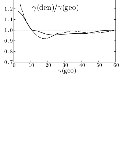
Figure 1: The ratios $\gamma(\mbox{den})/\gamma(\mbox{geo})$ are plotted as functions of $\gamma(\mbox{geo})$ for the cases of the Nilsson (solid line) and Woods-Saxon potentials (dashed line). The calculations have been performed for the TSD band in ¹⁶³Lu, and the parameters used for the Nilsson potential are $\epsilon_{2}=0.43$, $\epsilon_{4}=0.0$, and ${\mit\Delta}_{\rm n,p}=0.3$ MeV, and those for the Woods-Saxon potential are $\beta_{2}=0.42$, $\beta_{4}=0.034$, and ${\mit\Delta}_{\rm n,p}=0.3$ MeV, which has almost the same shape as the case of the Nilsson potential at $\gamma(\mbox{geo})\approx 10^{\circ}$ in the minimum of the Nilsson-Strutinsky calculation.

If the density is calculated within the mean-field approximation by using the average single-particle potential which has the same shape as the uniform density (5), then these two triaxiality parameters, $\gamma(\mbox{den})$ and $\gamma(\mbox{geo})$, agree very well. In Fig. 1 the ratio $\gamma(\mbox{den})/\gamma(\mbox{geo})$ is shown as a function of $\gamma(\mbox{geo})$, and we can see that they coincide typically within 10% except in the small $\gamma$ region, where both $\gamma(\mbox{den})$ and $\gamma(\mbox{geo})$ become zero and the ratio is numerically unstable. This agreement corresponds to the so-called shape consistency between the density and the potential Nerlo-Pomorska and Pomorski (1977), which has been tested both for the Nilsson and Woods-Saxon potentials for the axially symmetric deformations Dudek et al. (1984); Bengtsson et al. (1989). Therefore, we can practically use $\gamma(\mbox{geo})$ in place of $\gamma(\mbox{den})$.

The definition of triaxiality parameter, $\gamma(\mbox{den})$ or $\gamma(\mbox{geo})$, is basic or fundamental in the sense that it is directly related to the $B(E2)$ values of the triaxial rotor. In the microscopic calculations by means of the Hartree-Fock or Hartree-Fock-Bogoliubov method, $\gamma=\gamma(\mbox{den})$ is the only definition of the triaxial deformation, and no confusion exists. It is, however, quite often that one starts from some average nuclear potential, which is triaxially deformed, and calculates the potential energy surface or the total routhian surface to determine the selfconsistent deformation as in the case of the Strutinsky method. In such cases, a different type of definitions of the triaxiality parameter $\gamma$ has been used, which is chosen conveniently to specify the triaxial deformation of the potential. We call this third type of definition “$\gamma(\mbox{pot})$”: We consider two well-known definitions in the followings, depending on the employed potential.

II.2 $\gamma$(pot) defined in the Nilsson potential

As a definite example of $\gamma(\mbox{pot})$, we take the Nilsson potential, or the modified oscillator potential, as a mean-field potential, i.e. $\gamma(\mbox{pot:Nils})$. The deformation parameters in the Nilsson potential Nilsson et al. (1969); Bengtsson and Ragnarsson (1985); Nilsson and Ragnarsson (1995) considered in the present work are $(\epsilon_{2},\gamma,\epsilon_{4})$, which define the deformation of the velocity independent part of potential through the single-stretched coordinate, $\mbox{\boldmath$r$}^{\prime}\equiv(\sqrt{\omega_{x}/\omega_{0}}\,x,\sqrt{\omega_{y}/\omega_{0}}\,y,\sqrt{\omega_{z}/\omega_{0}}\,z)$, as

$$\begin{array}[]{l}{\displaystyle V(\mbox{\boldmath$r$})=\frac{1}{2}M\omega_{0}\omega_{\rm v}(\epsilon_{2},\gamma,\epsilon_{4})r^{\prime 2}\times\vspace{1mm}}\\ {\displaystyle\quad\Bigl{(}1-\sum_{K=0,\pm 2}c_{2K}Y_{2K}(\Omega^{\prime})-\sum_{K=0,\pm 2,\pm 4}c_{4K}Y_{4K}(\Omega^{\prime})\Bigr{)},}\end{array}$$ (6)

where $\omega_{0}$ is the frequency of the spherical potential, $\omega_{\rm v}(\epsilon_{2},\gamma,\epsilon_{4})$ is determined by the volume conserving condition, $\Omega^{\prime}$ is the solid-angle of coordinate $\mbox{\boldmath$r$}^{\prime}$, and the coefficients $c$’s are given by

$$\left\{\begin{array}[]{l}c_{20}=\sqrt{\frac{16\pi}{45}}\,\epsilon_{2}\cos\gamma,\\ c_{22}=c_{2-2}=-\sqrt{\frac{8\pi}{45}}\,\epsilon_{2}\sin\gamma,\\ c_{40}=\frac{\sqrt{4\pi}}{9}\,\epsilon_{4}(5\cos^{2}\gamma+1),\\ c_{42}=c_{4-2}=-\frac{\sqrt{120\pi}}{9}\,\epsilon_{4}\cos\gamma\sin\gamma,\\ c_{44}=c_{4-4}=\frac{\sqrt{70\pi}}{9}\,\epsilon_{4}\sin^{2}\gamma.\end{array}\right.$$ (7)

Note that the three frequencies, $\omega_{x}$, $\omega_{y}$, and $\omega_{z}$, are given by Eq. (9) below. The nuclear shape $\Sigma$ in this case is defined as an equi-potential surface of the potential, $V(\mbox{\boldmath$r$})=$ const., and is uniquely determined once the parameters $(\epsilon_{2},\gamma,\epsilon_{4})$ with $\gamma=\gamma(\mbox{pot:Nils})$ are given. It is straightforward but rather complicated because of the use of the single-stretched coordinate $\mbox{\boldmath$r$}^{\prime}$ in practice. Using this potential either the triaxiality parameter $\gamma(\mbox{den})$ or $\gamma(\mbox{geo})$ defined in the previous subsection can be calculated as functions of these potential parameters $(\epsilon_{2},\gamma=\gamma(\mbox{pot:Nils}),\epsilon_{4})$.

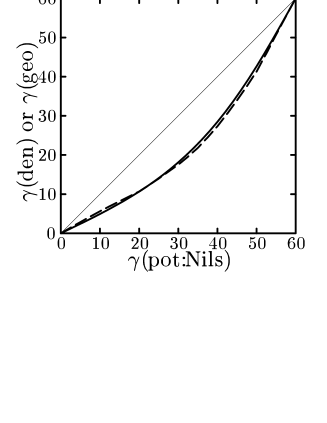
Figure 2: The triaxiality parameters $\gamma(\mbox{den})$ (dashed line) and $\gamma(\mbox{geo})$ (solid line) are shown as functions of the $\gamma$ parameter in the Nilsson potential, $\gamma(\mbox{pot:Nils})$ (the thin diagonal line is just for a guide to the eyes). The calculations have been performed for the TSD band in ¹⁶³Lu, and the parameters used are $\epsilon_{2}=0.43$, $\epsilon_{4}=0.0$, and ${\mit\Delta}_{\rm n,p}=0.3$ MeV.

Figure 3: The triaxiality parameters $\gamma(\mbox{geo})$ with fixed $\epsilon_{2}$ and $\epsilon_{4}$ deformation parameters are shown as functions of $\gamma(\mbox{pot:Nils})$ (the thin diagonal line is just for a guide to the eyes). The dotted line is for the case with $\epsilon_{2}=0.2$, the dashed with $\epsilon_{2}=0.4$, and the solid with $\epsilon_{2}=0.6$, respectively. The $\epsilon_{4}$ parameter is set 0 for all the cases.

In Fig. 2, are depicted the relation between $\gamma(\mbox{den})$ and $\gamma(\mbox{pot:Nils})$ and that between $\gamma(\mbox{geo})$ and $\gamma(\mbox{pot:Nils})$ at a given $(\epsilon_{2},\epsilon_{4})$, which is suitable for the TSD band in ¹⁶³Lu. As is already shown in Fig. 1, $\gamma(\mbox{den})$ and $\gamma(\mbox{geo})$ are very similar, but $\gamma(\mbox{pot:Nils})$ is quite different: $\gamma(\mbox{pot:Nils})=20^{\circ}$ corresponds to $\gamma(\mbox{den})\approx\gamma(\mbox{geo})\approx 11^{\circ}$, so that the difference can be as much as about a factor two. In order to see how the difference between $\gamma(\mbox{geo})$ and $\gamma(\mbox{pot:Nils})$ changes for different $\epsilon_{2}$ values, three cases with $\epsilon_{2}=0.2$, 0.4, 0.6 are shown in Fig. 3. It is clear that the difference becomes larger for larger $\epsilon_{2}$ deformations: $\gamma(\mbox{geo})$ is only about $10^{\circ}$ even though $\gamma(\mbox{pot:Nils})$ is put $30^{\circ}$ in the case of the superdeformed band, $\epsilon_{2}\approx 0.6$.

In the case of $\epsilon_{4}=0$, the Nilsson potential reduces to the anisotropic harmonic oscillator potential except for the $\mbox{\boldmath$l$}^{2}$ and $\mbox{\boldmath$l$}\cdot\mbox{\boldmath$s$}$ terms, which are irrelevant for the definition of the nuclear shape. It is instructive to consider such a case in order to understand the difference shown in Fig. 3. Then the shape is a volume-conserving ellipsoid defined by simple equations,

$$\sum_{i=1}^{3}\omega_{i}^{2}x_{i}^{2}=\mbox{const.},\quad\mbox{with}\quad\prod_{i=1}^{3}\omega_{i}=\omega_{0}^{3}.$$ (8)

The frequencies $\omega_{i}$ ($i=1,2,3$) for the $x$, $y$, $z$-directions, which are inversely proportional to the lengths of the ellipsoid along these axes, are given by

$$\omega_{i}=\omega_{\rm v}\left(1-\frac{2}{3}\epsilon_{2}\cos\Bigl{(}\gamma+\frac{2\pi}{3}i\Bigr{)}\right),\quad\gamma=\gamma(\mbox{pot:Nils}).$$ (9)

Therefore $\gamma(\mbox{geo})$ and $\gamma(\mbox{pot:Nils})$ are related through $\omega_{i}$ ($i=1,2,3$);

$$\tan\gamma(\mbox{geo})={\displaystyle\frac{\sqrt{3}\,(\omega_{y}^{-2}-\omega_{x}^{-2})}{2\omega_{z}^{-2}-\omega_{y}^{-2}-\omega_{x}^{-2}}},$$ (10)

$$\tan\gamma(\mbox{pot:Nils})={\displaystyle\frac{\sqrt{3}\,(\omega_{y}-\omega_{x})}{2\omega_{z}-\omega_{y}-\omega_{x}}},$$ (11)

which relate these two $\gamma$’s for a given value of $\epsilon_{2}$. In the limit of small deformation parameters, $\epsilon_{2}$,$|\gamma|\ll 1$, it is easy to confirm

$$\gamma(\mbox{geo})\approx\Bigl{(}1-\frac{3}{2}\epsilon_{2}\Bigr{)}\,\gamma(\mbox{pot:Nils}).$$ (12)

Namely, the slope of curves at the origin in Fig. 3 changes with $\epsilon_{2}$ with a rather large factor $\frac{3}{2}$, and this clearly explains that $\gamma(\mbox{geo})$ is smaller than $\gamma(\mbox{pot:Nils})$ more than a factor two when $\epsilon_{2}$ is as large as 0.4 like in the case of the TSD band.

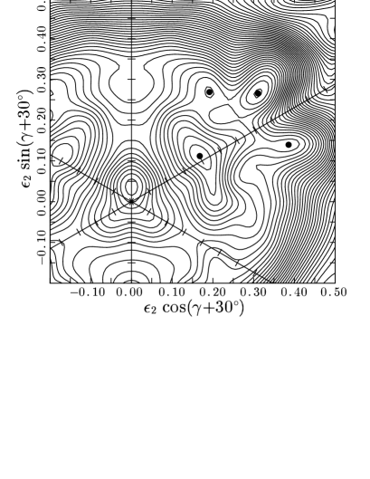
Figure 4: Potential energy surface obtained by the cranked Nilsson Strutinsky calculation for the $(\pi,\alpha)=(+,+1/2)$ configuration in ¹⁶³Lu at $I=41/2^{+}$. The energy between contours is 250 keV. The triaxiality parameter $\gamma=\gamma(\mbox{pot:Nils})$ is used as usual in the upper panel, while the triaxiality parameter $\gamma=\gamma(\mbox{geo})$ in the lower panel.

In order to see how these different definitions of two triaxiality parameters, $\gamma(\mbox{geo})$ and $\gamma(\mbox{pot:Nils})$, change the appearance of potential energy surface, we show an example in Fig. 4. Here the $\epsilon_{4}$ parameter is chosen to minimize the potential energy at each $(\epsilon_{2},\gamma)$ mesh points. The parameter $\gamma(\mbox{geo})$ depends not only on $(\epsilon_{2},\gamma(\mbox{pot:Nils}))$ but on $\epsilon_{4}$, and it is impossible to calculate the $(\epsilon_{2},\gamma(\mbox{geo}))$ mesh points before the minimization with respect to $\epsilon_{4}$. Therefore, we made an approximation to set $\epsilon_{4}=0$ when we prepare the $(\epsilon_{2},\gamma(\mbox{geo}))$ mesh points from the $(\epsilon_{2},\gamma(\mbox{pot:Nils}))$ mesh points. As is clear from the figure, the surface is squeezed to the $\gamma=0$ axis at larger deformation, and apparently the TSD minimum moves to smaller triaxial values. In Fig. 4, only the $\gamma$ parameter is replaced from $\gamma(\mbox{pot:Nils})$ to $\gamma(\mbox{geo})$. However, it may be better to replace $\epsilon_{2}$ to the other parameter corresponding to the magnitude $Q$ in Eq.(2) in order to make the meaning of the quadrupole deformation clearer. Constraint Hartree-Fock(-Bogoliubov) type calculations are necessary for such a purpose. Then the method becomes much more involved and the simplicity of the Strutinsky type calculation may be lost.

It may be worthwhile mentioning, here, the specific model composed of the spherical Nilsson potential and the $QQ$ force as an effective interaction. The velocity-independent part of the Hartree potential in this model is given by

$$\begin{array}[]{l}{\displaystyle V(\mbox{\boldmath$r$})=\frac{1}{2}M\omega_{0}^{2}\,\mbox{\boldmath$r$}^{2}-\alpha_{20}{\hat{Q}}_{20}-\alpha_{22}({\hat{Q}}_{22}+{\hat{Q}}_{2-2}),}\end{array}$$ (13)

where the Hartree condition requires $\alpha_{2K}=\chi\,\langle{\hat{Q}}_{2K}\rangle$ ($K=0,2$) with $\chi$ being the $QQ$ force strength, and the potential reduces also to the anisotropic harmonic oscillator (but the volume conservation condition is not necessarily satisfied in this Hartree procedure). If the model space is not restricted, $\alpha_{2K}$ is proportional to the two intrinsic quadrupole moments in Eq. (1), and then, the triaxiality parameter of the density type (3) in this case is related to $-\sqrt{2}\,\alpha_{22}/\alpha_{20}$, which can be expressed in terms of $\omega_{i}$ ($i=1,2,3$) as

$$\tan\gamma(\mbox{den:QQ})={\displaystyle\frac{\sqrt{3}\,(\omega_{y}^{2}-\omega_{x}^{2})}{2\omega_{z}^{2}-\omega_{y}^{2}-\omega_{x}^{2}}}.$$ (14)

It is usual to parametrize the potential by the deformation parameter $(\delta,\gamma)$ with $\gamma=\gamma(\mbox{den:QQ}))$, in terms of which the frequencies are written in the form,

$$\omega_{i}^{2}=\omega_{0}^{2}\left(1-\frac{4}{3}\delta\cos\Bigl{(}\gamma+\frac{2\pi}{3}i\Bigr{)}\right),\quad\gamma=\gamma(\mbox{den:QQ}).$$ (15)

Thus, the triaxiality parameters $\gamma(\mbox{geo})$ and $\gamma(\mbox{den:QQ})$ are quite different in this case: In the limit of small deformation parameters, $\delta$,$|\gamma|\ll 1$, they are related like

$$\gamma(\mbox{geo})\approx(1-2\delta)\,\gamma(\mbox{den:QQ}).$$ (16)

Namely, the difference is even larger than that between $\gamma(\mbox{geo})$ and $\gamma(\mbox{pot:Nils})$. This means that the shape consistency between the density and the potential is strongly violated in the $QQ$ force model, if the full model space is used in the Hartree procedure. Considering this on top of the fact that the volume conservation condition is not guaranteed, the model is not realistic at all.

Actually, the $QQ$ force model is supposed to be a model in a restricted model space, and the contributions of the “core” should be added to $\langle{\hat{Q}}_{2K}\rangle$ calculated within the model space in order to obtain the intrinsic moments of the whole system. Then the problem of breaking the shape consistency may not be the real problem. In fact, the core contributions of the quadrupole operators, i.e. the expectation values for the closed shell configurations in the anisotropic harmonic oscillator potential, have different dependence on the deformation; it can be shown Y. R. Shimizu and K. Matsuyanagi (1984b) that they lead to the triaxiality parameter $\gamma=\gamma(\mbox{den:core})$, which satisfies

$$\tan\gamma(\mbox{den:core})={\displaystyle\frac{\sqrt{3}\,(\omega_{y}^{-1}-\omega_{x}^{-1})}{2\omega_{z}^{-1}-\omega_{y}^{-1}-\omega_{x}^{-1}}}.$$ (17)

In Ref. Y. R. Shimizu and K. Matsuyanagi (1984b) (see Appendix B of this reference for details, but note the different notations used there), these differences between various types of the deformation parameters defined in the harmonic oscillator potential were already discussed, where not only the parameter $\gamma$ but also the other one of a pair of the parameters, $\beta=\sqrt{\frac{4\pi}{5}}\,Q/\langle\sum_{k=1}^{A}\mbox{\boldmath$r$}^{2}\rangle$, were considered. It was already pointed out that the triaxiality parameters for a given shape in various types of definition take quite different values.

II.3 $\gamma$(pot) defined in the Woods-Saxon potential

As an another example of $\gamma(\mbox{pot})$, the parametrization of deformation in the Woods-Saxon potential is considered, i.e. $\gamma(\mbox{pot:WS})$. Actually, it is not restricted to the Woods-Saxon potential, but is more general as one can see in the following. The deformed Woods-Saxon potential considered in this work is parametrized by the deformation parameters, $(\beta_{2},\gamma,\beta_{4})$, and defined Dudek et al. (1979); Rohozinski and Sobiczewski (1981); Nazarewicz and Sobiczewski (1981) by

$${\displaystyle V(\mbox{\boldmath$r$})=\frac{V_{0}}{1+\exp(\mbox{dist}_{\Sigma}(\mbox{\boldmath$r$})/a)}},$$ (18)

where $\mbox{dist}_{\Sigma}(\mbox{\boldmath$r$})$ is the distance between a given point $r$ and the nuclear surface $\Sigma$, with a minus sign if $r$ is inside $\Sigma$, which is defined by the usual radius to solid-angle relation, $r=R(\Omega)$;

$$\begin{array}[]{l}{\displaystyle R(\Omega)=R_{\rm v}(\beta_{2},\gamma,\beta_{4})\times\vspace{1mm}}\\ {\displaystyle\quad\Bigl{(}1+\sum_{K=0,\pm 2}a_{2K}Y_{2K}(\Omega)+\sum_{K=0,\pm 2,\pm 4}a_{4K}Y_{4K}(\Omega)\Bigr{)},}\end{array}$$ (19)

where $R_{\rm v}(\beta_{2},\gamma,\beta_{4})$ is determined by the volume conserving condition, and the coefficients $a$’s are given by

$$\left\{\begin{array}[]{l}a_{20}=\beta_{2}\cos\gamma,\\ a_{22}=a_{2-2}=-\frac{1}{\sqrt{2}}\,\beta_{2}\sin\gamma,\\ a_{40}=\frac{1}{6}\,\beta_{4}(5\cos^{2}\gamma+1),\\ a_{42}=a_{4-2}=-\sqrt{\frac{5}{6}}\,\beta_{4}\cos\gamma\sin\gamma,\\ a_{44}=a_{4-4}=\sqrt{\frac{35}{72}}\,\beta_{4}\sin^{2}\gamma.\end{array}\right.$$ (20)

Apparently the surface $\Sigma$ is given as an equi-potential surface at the half depth, $V(\mbox{\boldmath$r$})=\frac{1}{2}V_{0}$, and it is directly related to $(\beta_{2},\gamma,\beta_{4})$ with $\gamma=\gamma(\mbox{pot:WS})$.

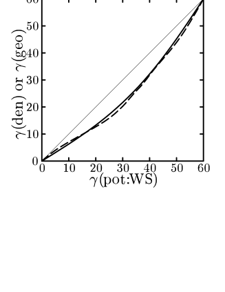
Figure 5: The triaxiality parameters $\gamma(\mbox{den})$ (dashed line) and $\gamma(\mbox{geo})$ (solid line) are shown as functions of the $\gamma$ parameter in the Woods-Saxon potential, $\gamma(\mbox{pot:WS})$ (the thin diagonal line is just for a guide to the eyes). The calculations have been performed for the TSD band in ¹⁶³Lu, and the parameters used are $\beta_{2}=0.42$, $\beta_{4}=0.034$, and ${\mit\Delta}_{\rm n,p}=0.3$ MeV; these deformation parameters gives almost the same shape as that used in the Nilsson potential in Fig. 2 at $\gamma(\mbox{geo})\approx 10^{\circ}$.

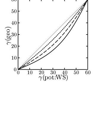
Figure 6: The triaxiality parameters $\gamma(\mbox{geo})$ with fixed $\beta_{2}$ and $\beta_{4}$ deformation parameters are shown as functions of $\gamma(\mbox{pot:WS})$ (the thin diagonal line is just for a guide to the eyes). The dotted line is for the case with $\beta_{2}=0.217$ and $\beta_{4}=0.017$, the dashed with $\beta_{2}=0.445$ and $\beta_{4}=0.075$, and the solid with $\beta_{2}=0.685$ and $\beta_{4}=0.190$, respectively. These sets of parameters almost correspond to the cases of $\epsilon_{2}=0.2$, $\epsilon_{2}=0.4$, and $\epsilon_{2}=0.6$ with $\epsilon_{4}=0$ used for the Nilsson potential in Fig. 3 at $\gamma(\mbox{geo})=0$.

As in the case of the Nilsson potential, the triaxiality parameter $\gamma(\mbox{den})$ and $\gamma(\mbox{geo})$ are shown as functions of $\gamma(\mbox{pot:WS})$ in Fig. 5, which are suitable to the TSD band in ¹⁶³Lu, just in the same way as in the case of the Nilsson potential in Fig. 2. Again, $\gamma(\mbox{den})$ and $\gamma(\mbox{geo})$ are very similar, but they are quite different from $\gamma(\mbox{pot:WS})$: $\gamma(\mbox{den})\approx\gamma(\mbox{geo})\approx 13^{\circ}$ when $\gamma(\mbox{pot:WS})=20^{\circ}$. In Fig. 6, the relation between $\gamma(\mbox{geo})$ and $\gamma(\mbox{pot:WS})$ at three different cases of $(\beta_{2},\beta_{4})$ deformations, corresponding to Fig. 3, are also depicted. Although the differences between $\gamma(\mbox{geo})$ and $\gamma(\mbox{pot:WS})$ are not so dramatic as those between $\gamma(\mbox{geo})$ and $\gamma(\mbox{pot:Nils})$, they are still considerably large. In the case of the parametrization of the nuclear surface in Eq. (19), $\langle{\hat{Q}}_{2K}\rangle_{\rm uni}$ can be easily calculated;

$$\langle{\hat{Q}}_{2K}\rangle_{\rm uni}=\frac{1}{5}\int R(\Omega)^{5}Y_{2K}(\Omega)d\Omega.$$ (21)

Then, it is straightforward to see, in the small deformation limit, $\beta_{2}$,$|\gamma|\ll 1$, with $\beta_{4}=0$, that

$$\gamma(\mbox{geo})\approx\Bigl{(}1-\sqrt{\frac{180}{49\pi}}\,\beta_{2}\Bigr{)}\,\gamma(\mbox{pot:WS}).$$ (22)

Taking into account the relation, $\beta_{2}\approx\sqrt{\frac{16\pi}{45}}\,\epsilon_{2}$ in the small deformation limit, the proportionality constant in front of $\epsilon_{2}$ corresponds, in this case, to $\sqrt{\frac{180}{49\pi}}\times\sqrt{\frac{16\pi}{45}}=\frac{8}{7}\approx 1.14$, which is smaller than $\frac{3}{2}=1.5$ in Eq. (12) for the Nilsson potential, but is still appreciably large. This explains qualitatively the increase of the difference between $\gamma(\mbox{geo})$ and $\gamma(\mbox{pot:WS})$ for larger deformations as is shown in Fig. 6.

III $B(E2)$ ratio of the wobbling band

As it is discussed in the previous section, the two intrinsic quadrupole moments should be determined in order to deduce the triaxial deformation. In the case of the wobbling excitations, it is enough to measure the two $B(E2)$’s, $B(E2)_{\rm in}$ and $B(E2)_{\rm out}$; the ${\mit\Delta}I=-2$ intraband $E2$ transitions within the wobbling band and ${\mit\Delta}I=\pm 1$ interband $E2$ transitions from the one-phonon wobbling band to the yrast TSD band, respectively. According to the rotor model Bohr and Mottelson (1975), the magnitude of the moment $Q$ in Eq.(2) is factored out in the two $B(E2)$’s and their ratio, $B(E2)_{\rm out}/B(E2)_{\rm in}$, is directly related to the triaxiality parameter $\gamma(\mbox{den})$. This $B(E2)$ ratio is straightforward to measure from the experimental point of view; it is given directly by the $\gamma$-ray branching ratio if the information of the mixing ratio is provided. In contrast, the life time measurement is necessary to obtain $B(E2)$ values themselves, which is not an easy task generally. Although the life time measurements have been done in some TSD bands Schönwaßer et al. (2002); Görgen et al. (2004) recently, so that we can study both $B(E2)_{\rm out}$ and $B(E2)_{\rm in}$ separately, we concentrate upon the $B(E2)$ ratio in the present work.

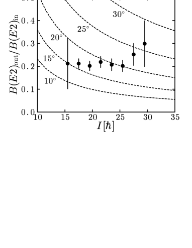
Figure 7: The $B(E2)$ ratio, $B(E2\mbox{:}\,I\rightarrow I-1)_{\rm out}/B(E2\mbox{:}\,I\rightarrow I-2)_{\rm in}$, of the wobbling band in ¹⁶³Lu. The experimental data Görgen et al. (2004) is compared with the calculations by the particle-rotor model I. Hamamoto and G. B. Hagemann (2003). Five dotted curves are the results with the triaxiality parameter $\gamma(\mbox{den})=10^{\circ}$, $15^{\circ}$, $20^{\circ}$, $25^{\circ}$, and $30^{\circ}$ from the lowest to the highest ones, respectively.

In Fig. 7, the experimental $B(E2)$ ratio of the one-phonon wobbling band in ¹⁶³Lu Görgen et al. (2004) is compared with the results of the particle-rotor model calculation in Ref. I. Hamamoto and G. B. Hagemann (2003). Important parameters of the model are three moments of inertia, ${\cal J}_{x}$, ${\cal J}_{y}$, ${\cal J}_{z}$, and the triaxiality $\gamma=\gamma(\mbox{den})$; an overall factor of the formers is irrelevant to the $B(E2)$ ratio and they are fixed to be ${\cal J}_{x}:{\cal J}_{y}:{\cal J}_{z}=145:135:50$ taken from I. Hamamoto and G. B. Hagemann (2003), while we take five values $\gamma(\mbox{den})=10^{\circ}$, $15^{\circ}$, $20^{\circ}$, $25^{\circ}$, and $30^{\circ}$ in order to show the dependence of the $B(E2)$ ratio on the $\gamma$ values. Other parameters, the chemical potential of the odd $i_{13/2}$ proton, $\lambda/\kappa=-1.532$, and the pairing gap, $\Delta/\kappa=0.3$, with $\kappa=3$ MeV are also taken from I. Hamamoto and G. B. Hagemann (2003). The calculated ratios are monotonically decreasing functions of spin if all the model parameters are held fixed. This decrease is characteristic in the rotor model, see Eq. (23) below. Although the spin-dependence is somewhat different, the average value of the $B(E2)$ ratio can be reproduced if we take the value $\gamma\approx 20^{\circ}$. Therefore the triaxial deformation of ¹⁶³Lu is deduced to be $\gamma\approx 20^{\circ}$, which is one of the main conclusions of Ref. I. Hamamoto and G. B. Hagemann (2003). This conclusion remains valid even if the parameters of the moments of inertia are changed in a reasonable range. While the existence of the odd proton brings about important corrections to the energy spectra, its effect on the $B(E2)$ is very small I. Hamamoto and G. B. Hagemann (2003); K. Tanabe and K. Sugawara-Tanabe (2006). Thus, the wobbling phonon treatment of the simple rotor model in Ref. Bohr and Mottelson (1975) gives a good approximation to the $B(E2)$ ratio at high-spin states, leading to the following expression;

$$\begin{array}[]{l}{\displaystyle\frac{B(E2\mbox{:}\,I\rightarrow I\pm 1)_{\rm out}}{B(E2\mbox{:}\,I\rightarrow I-2)_{\rm in}}\vspace{1mm}}\\ \quad\approx{\displaystyle\frac{2}{I}\left(\frac{w_{z}\sin(\gamma+60^{\circ})\mp w_{y}\sin{\gamma}}{\sqrt{w_{y}w_{z}}\cos(\gamma+30^{\circ})}\right)^{2},\quad\gamma=\gamma(\mbox{den})},\end{array}$$ (23)

where the quantities $w_{y},w_{z}$ are related to the three moments of inertia through

$$\left\{\begin{array}[]{l}w_{y}\equiv({\cal J}_{x}/{\cal J}_{z}-1)^{1/2},\\ w_{z}\equiv({\cal J}_{x}/{\cal J}_{y}-1)^{1/2}.\end{array}\right.$$ (24)

Note that the $I\rightarrow I+1$ transitions are quenched for the positive $\gamma$ shape, and in fact only the $I\rightarrow I-1$ transitions are observed in experiment in the Lu nuclei. It is easy to check that the results of calculations in Fig. 7 can be understood nicely by this simple expression; the decrease of the $B(E2)$ ratio as a function of spin is due to the $1/I$ dependence in Eq.(23), and the ratio increases quickly as a function of the triaxiality $\gamma=\gamma(\mbox{den})$.

It may be interesting to note that the measured $B(E2)$ ratio is almost constant as a function of spin or even increases at highest spins, which is quite different from that of the rotor model calculation. It indicates that the parameters of the model are changing as the spin $I$ increases. Since the ratio is sensitive to the triaxiality parameter $\gamma=\gamma(\mbox{den})$, it is natural to consider that $\gamma(\mbox{den})$ is spin dependent and increases with spins I. Hamamoto and G. B. Hagemann (2003) among others. A preliminary investigation for such a possibility has been reported in Ref. Shoji and Shimizu (2006), where is employed a microscopic framework, the cranked Woods-Saxon mean-field and the random phase approximation (RPA).

Next let us turn to the discussion on our microscopic calculations in Refs. Matsuzaki et al. (2002); Matsuzaki et al. (2004b, a), which are based on the cranked Nilsson mean-field and the random phase approximation (RPA). In these calculations the triaxiality parameter $\gamma=20^{\circ}$ was employed but the resultant $B(E2)$ ratios were too small by a factor two to three. We were wondering about possible reasons; does the results of RPA calculation deviate from those of the rotor model so much? However, it has been shown in Ref. Shimizu et al. (2005) that the RPA calculation reproduces the result of the rotor model rather well in the case of the precession bands, which are nothing but the rotational bands built upon the high-$K$ isomers and can be interpreted as a similar motion to the wobbling excitation, where the angular momentum vector fluctuates about the main rotation axis Andersson et al. (1976). Now the reason of the small calculated $B(E2)$ ratio is clear from the argument of the previous section: The triaxiality $\gamma$ used in our calculations is that of the Nilsson potential, $\gamma(\mbox{pot:Nils})$, in §II.2, while the $\gamma$ used in the rotor model is $\gamma(\mbox{den})$ in §II.1. As is discussed in the previous section, the difference between them for the same shape is very large for large deformations like in the case of the TSD bands; $\gamma(\mbox{pot:Nils})\approx 20^{\circ}$ corresponds to $\gamma(\mbox{den})\approx 11^{\circ}$, and in order to perform the same calculation as the rotor model with $\gamma(\mbox{den})\approx 20^{\circ}$ one has to employ $\gamma(\mbox{pot:Nils})\approx 30^{\circ}$ according to Fig. 2. It should also be mentioned that we have used five major oscillator shells, $N_{\rm osc}=3-5$ for proton and $N_{\rm osc}=4-8$ for neutron in the calculation in Refs. Matsuzaki et al. (2002); Matsuzaki et al. (2004b, a), which were not enough; since the $i_{13/2}$ proton orbits are occupied in the TSD band, the inclusion of $N_{\rm osc}=8$ proton quasiparticle states are necessary in the RPA calculational step.

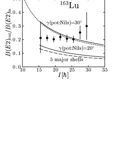
Figure 8: The $B(E2)$ ratio, $B(E2\mbox{:}\,I\rightarrow I-1)_{\rm out}/B(E2\mbox{:}\,I\rightarrow I-2)_{\rm in}$, of the one-phonon wobbling band in ¹⁶³Lu. The experimental data Görgen et al. (2004) is compared with the calculations by our microscopic RPA approach. The lower solid line is the result with $\gamma=\gamma(\mbox{pot:Nils})=20^{\circ}$, while the upper solid line is with $\gamma(\mbox{pot:Nils})=30^{\circ}$; the full model space is used for both of them. The dashed line is the result with $\gamma(\mbox{pot:Nils})=20^{\circ}$ and using only the five major oscillator shells, corresponding to the previous calculation in Ref. Matsuzaki et al. (2002). The dotted line is the same as that in Fig. 7, the particle-rotor calculation with $\gamma=\gamma(\mbox{den})=20^{\circ}$, depicted for a reference.

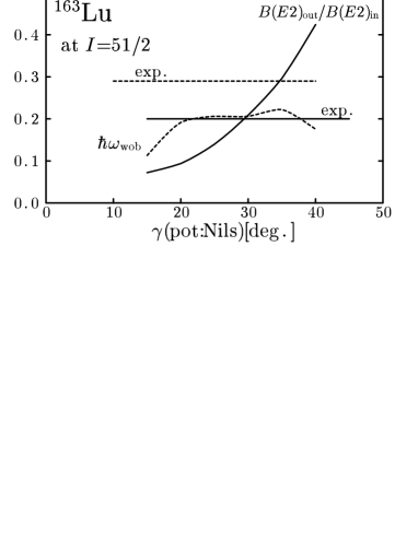
Figure 9: The $\gamma$ dependence of the microscopically calculated $B(E2)$ ratio and the excitation energy of the one-phonon wobbling band in ¹⁶³Lu at spin $I=51/2$. The solid lines are the $B(E2)$ ratios and the dotted lines are the energy in MeV. The horizontal solid and dotted lines designate the experimental values.

In Fig. 8 we depict the new results of calculation employing $\gamma(\mbox{pot:Nils})=20^{\circ}$ and $30^{\circ}$ with using the full model space; all orbits in the oscillator shell $N_{\rm osc}=0-9$ for both protons and neutrons are included. The procedure and the other parameters in the calculation are the same as in the previous work Matsuzaki et al. (2002); $\epsilon_{2}=0.43$, $\epsilon_{4}=0$, and the pairing gaps ${\mit\Delta}_{\rm n,p}=0.3$ MeV. The result of the previous calculation, the dashed line, and that of the particle-rotor model with $\gamma(\mbox{den})=20^{\circ}$, the dotted line, are also included. Our previous calculation is smaller than the experimental data partly because of the small model space, but its effect is about 20%; the large difference is mainly due to the fact that we have used $\gamma=\gamma(\mbox{pot:Nils})=20^{\circ}$ in the previous calculation, which corresponds to much smaller triaxiality than $\gamma(\mbox{den})=20^{\circ}$ in the particle-rotor model. The result with $\gamma(\mbox{pot:Nils})=30^{\circ}$ almost coincides with that of the particle-rotor calculation using $\gamma(\mbox{den})=20^{\circ}$, because the values ${\cal J}_{x}:{\cal J}_{y}:{\cal J}_{z}$ of the microscopically calculated moments of inertia accidentally take similar values in the relevant spin range Matsuzaki et al. (2002). In order to see the $\gamma$ dependence of the results, we show, in Fig. 9, the $B(E2)$ ratio and the excitation energy of the one-phonon wobbling band in ¹⁶³Lu at spin $I=51/2$ as functions of the triaxiality $\gamma=\gamma(\mbox{pot:Nils})$. Although the excitation energy is rather flat in the range, $20^{\circ}\leq\gamma(\mbox{pot:Nils})\leq 30^{\circ}$, the $B(E2)$ follows the behaviors of Eq. (23) if the relation between $\gamma(\mbox{pot:Nils})$ and $\gamma(\mbox{den})$ is taken into account. The excitation energy can be expressed in terms of the three moments of inertia in an usual way Bohr and Mottelson (1975); Marshalek (1979), but their $\gamma$ dependences are not simple like the irrotational one Shimizu and Matsuzaki (1995) and lead to a rather weak $\gamma$ dependence of the excitation energy in this case. Here we have only shown the example of the wobbling excitation in ¹⁶³Lu, but we have confirmed that these properties of the wobbling-like RPA solution are general, and can be applied for other cases in the Lu region.

Thus, our microscopic RPA calculations give more or less the same results as that of the macroscopic particle-rotor model, if the corresponding magnitude of the triaxial deformation is employed. It shows that the RPA calculation of the wobbling excitation in the Lu region leads to the behaviors of $B(E2)$’s that are given by the macroscopic rotor model; namely the out-of-band $B(E2)$ can be related to the static triaxial deformation. This is non trivial since the out-of-band $B(E2)$ is calculated by the RPA transition amplitudes of the non-diagonal part of the quadrupole operators, $Q_{21}^{(-)}$ and $Q_{22}^{(-)}$ Marshalek (1977, 1979). It has been shown Shimizu and Matsuzaki (1995) that the RPA wobbling theory of Marshalek Marshalek (1979) gives the same expression of the out-of-band $B(E2)$ as that of the rotor model, if the RPA wobbling mode is collective enough that the quantity “$c_{n}$” defined in Eq. (4.29) in Ref. Shimizu and Matsuzaki (1995) satisfies $c_{n={\rm wob}}=1$. In the previous calculations Shimizu and Matsuzaki (1995); Matsuzaki et al. (2002); Matsuzaki et al. (2004b, a), the employed model space was too small  to give $c_{n={\rm wob}}=1$, but we have confirmed that $c_{n={\rm wob}}\approx 1$ is satisfied within 1% in the present full model space calculations. Recently, this criterion, $c_{n={\rm wob}}\approx 1$, has been used to identify the wobbling-like solution out of many RPA eigenmodes, and shown to be very useful Kvasil and Nazmitdinov (2007).

IV Summary

In this work, we have first discussed the differences of the various definitions of the triaxiality parameter $\gamma$. The most basic among them is defined through the two intrinsic quadrupole moments, $\gamma(\mbox{den})$ in Eq. (3) for each configuration of a particular nucleus, or $\gamma(\mbox{geo})$ in Eq. (4) for a given nuclear shape. It has been found that these two coincide in a good approximation (the nuclear shape consistency). In the Hartree-Fock(-Bogoliubov) type calculations, where the nuclear mean-field is determined selfconsistently by a suitably chosen effective interaction, the parameter $\gamma(\mbox{den})$ is the only possible definition of triaxial deformation. However, there is an another type of mean-field calculations, i.e. the Strutinsky macroscopic-microscopic method, where one starts from a suitably chosen average potential, in which the nuclear deformation is parametrized in various different ways. We have considered the two widely adopted ones, the Nilsson type and the Woods-Saxon type parametrizations. The triaxiality parameters associated with these potentials, $\gamma(\mbox{pot:Nils})$ in Eqs. (6)-(7) and $\gamma(\mbox{pot:WS})$ in Eqs. (18)-(19), are compared with the density type $\gamma(\mbox{den})$ and $\gamma(\mbox{geo})$. Conspicuous differences between the potential type and the density type $\gamma$’s, e.g. $\gamma(\mbox{pot:Nils})$ vs. $\gamma(\mbox{geo})$, have been found especially for larger deformations, e.g. the triaxial superdeformed states. It is also investigated how the differences between various definitions come out by evaluating their relations explicitly in the small deformation limit. Therefore we have to be very careful about which definition is used in quantitative discussions of the triaxial deformation.

Next, we have investigated the out-of-band to in-band $B(E2)$ ratio of the one-phonon wobbling band, which is measured systematically in the Lu region and is sensitive to the triaxial deformation. The macroscopic particle-rotor model I. Hamamoto and G. B. Hagemann (2003) is used to deduce the triaxial deformation from the experimental $B(E2)$ ratio, which leads to $\gamma=\gamma(\mbox{den})\approx 20^{\circ}$ on average. On the other hand, we performed the microscopic RPA calculation Matsuzaki et al. (2002); Matsuzaki et al. (2004a) with using $\gamma=\gamma(\mbox{pot:Nils})\approx 20^{\circ}$ corresponding to the TSD minima in the cranked Nilsson-Strutinsky calculation Schnack-Petersen et al. (1995); Bengtsson , but we obtained too small $B(E2)$ ratio compared with the experimental data. It has been found that the reason of the underestimation of our previous microscopic calculation is mainly due to the different triaxial deformation used: We have used $\gamma(\mbox{pot:Nils})\approx 20^{\circ}$ corresponding roughly to $\gamma(\mbox{den})\approx 11^{\circ}$, which is much smaller than $\gamma(\mbox{den})\approx 20^{\circ}$ in the rotor model calculations. If the proper triaxiality corresponding to $\gamma(\mbox{den})\approx 20^{\circ}$ is used, our RPA calculation can nicely reproduce the magnitude of the measured $B(E2)$ ratio in the same way as in the macroscopic particle-rotor model.

It should, however, be emphasized that an important problem remains: The predicted triaxial deformations, $\gamma(\mbox{den})\approx 11^{\circ}$, by the cranked Nilsson-Strutinsky calculations Schnack-Petersen et al. (1995); Bengtsson for the TSD bands in the Hf, Lu region are too small to account for the measured $B(E2)$ ratio of the wobbling excitations. We believe that this is a challenge to the existing microscopic theory. An another thing we would like to mention is that the measured $B(E2)$, both the out-of-band and in-band $B(E2)$’s, seems to indicate that the triaxial deformation is changing as a function of spin; it increases at higher spins I. Hamamoto and G. B. Hagemann (2003). We have recently developed a new RPA approach Shoji and Shimizu (2006) based on the Woods-Saxon potential as a mean-field, which is believed to be more reliable than our previous calculations employing the Nilsson potential. The result of calculations and discussions including the issue of the change of the triaxial deformation suggested by the out-of-band as well as in-band $B(E2)$’s will be reported in a subsequent paper; see Ref. Shoji and Shimizu (2006) for a preliminary report.

References

- Davydov and Filippov (1958) A. S. Davydov and B. F. Filippov, Nucl. Phys. A 8, 237 (1958).
- Meyer-ter-Vehn (1975) J. Meyer-ter-Vehn, Nucl. Phys. A 249, 111, 141 (1975).
- Cline (1986) D. Cline, Ann. Rev. Nucl. Part. Sci. 36, 683 (1986).
- Andrejtscheff and Petkov (1994) W. Andrejtscheff and P. Petkov, Phys. Lett. B 329, 1 (1994).
- Hamamoto (1989) I. Hamamoto, in Proc. of the Workshop on Microscopic Models in Nuclear Structure Physics, Oak Ridge, USA, Oct. 3 - 6, 1988, edited by M. W. Guidry et al. (World Scientific, 1989), p. 173.
- Hamamoto (1990) I. Hamamoto, Nucl. Phys. A 520, 297c (1990).
- Bohr and Mottelson (1975) A. Bohr and B. R. Mottelson, Nuclear Structure Vol. II (Benjamin, New York, 1975).
- S. W. Ødegård et al. (2001) S. W. Ødegård et al., Phys. Rev. Lett. 86, 5866 (2001).
- D. R. Jensen et al. (2002) D. R. Jensen et al., Nucl. Phys. A 703, 3 (2002).
- D. R. Jensen et al. (2004) D. R. Jensen et al., Eur. Phys. J. A 19, 173 (2004).
- Jensen et al. (2002) D. R. Jensen et al., Phys. Rev. Lett. 89, 142503 (2002).
- Schönwaßer et al. (2003) G. Schönwaßer et al., Phys. Lett. B 552, 9 (2003).
- Amro et al. (2003) H. Amro et al., Phys. Lett. B 553, 197 (2003).
- Bringel et al. (2005) P. Bringel et al., Eur. Phys. J. A 24, 167 (2005).
- Ragnarsson (1989) I. Ragnarsson, Phys. Rev. Lett. 62, 2084 (1989).
- Åberg (1990) S. Åberg, Nucl. Phys. A 520, 35c (1990).
- (17) R. Bengtsson, http://www.matfys.lth.se/ragnar/TSD.html.
- Nilsson and Ragnarsson (1995) S. G. Nilsson and I. Ragnarsson, Shapes and Shells in Nuclear Structure (Cambridge University Press, 1995).
- Schnack-Petersen et al. (1995) H. Schnack-Petersen et al., Nucl. Phys. A 594, 175 (1995).
- Schönwaßer et al. (2002) G. Schönwaßer et al., Eur. Phys. J. A 15, 435 (2002).
- Görgen et al. (2004) A. Görgen et al., Phys. Rev. C 69, 031301(R) (2004).
- I. Hamamoto (2002) I. Hamamoto, Phys. Rev. C 65, 044305 (2002).
- I. Hamamoto and G. B. Hagemann (2003) I. Hamamoto and G. B. Hagemann, Phys. Rev. C 67, 014319 (2003).
- Casten et al. (2003) R. F. Casten, E. A. McCutchan, N. V. Zamfir, C. W. Beausang, and J. ye Zhang, Phys. Rev. C 67, 064306 (2003).
- Matsuzaki et al. (2002) M. Matsuzaki, Y. R. Shimizu, and K. Matsuyanagi, Phys. Rev. C 65, 041303(R) (2002).
- Matsuzaki et al. (2004a) M. Matsuzaki, Y. R. Shimizu, and K. Matsuyanagi, Eur. Phys. J. A 20, 180 (2004a).
- Matsuzaki et al. (2004b) M. Matsuzaki, Y. R. Shimizu, and K. Matsuyanagi, Phys. Rev. C 69, 034325 (2004b).
- Marshalek (1977) E. R. Marshalek, Nucl. Phys. A 275, 416 (1977).
- Janssen and Mikhailov (1979) D. Janssen and I. N. Mikhailov, Nucl. Phys. A 318, 390 (1979).
- Marshalek (1979) E. R. Marshalek, Nucl. Phys. A 331, 429 (1979).
- J. L. Egido et al. (1980) J. L. Egido, H. J. Mang, and P. Ring, Nucl. Phys. A 339, 390 (1980).
- Y. R. Shimizu and K. Matsuyanagi (1983) Y. R. Shimizu and K. Matsuyanagi, Prog. Theor. Phys. 70, 144 (1983).
- Y. R. Shimizu and K. Matsuyanagi (1984a) Y. R. Shimizu and K. Matsuyanagi, Prog. Theor. Phys. 72, 799 (1984a).
- Kvasil and Nazmitdinov (2004) J. Kvasil and R. G. Nazmitdinov, Phys. Rev. C 69, 031304(R) (2004).
- Kvasil and Nazmitdinov (2006) J. Kvasil and R. G. Nazmitdinov, Phys. Rev. C 73, 014312 (2006).
- Matsuzaki (1990) M. Matsuzaki, Nucl. Phys. A 509, 269 (1990).
- Shimizu and Matsuzaki (1995) Y. R. Shimizu and M. Matsuzaki, Nucl. Phys. A 588, 559 (1995).
- Kvasil and Nazmitdinov (2007) J. Kvasil and R. G. Nazmitdinov, Phys. Lett. B 650, 331 (2007).
- Almehed et al. (2006) D. Almehed, R. G. Nazmitdinov, and F. Dönau, Phys. Script. T125, 139 (2006).
- Shimizu et al. (2006) Y. R. Shimizu, M. Matsuzaki, and K. Matsuyanagi, Phys. Script. T125, 134 (2006).
- Shoji and Shimizu (2006) T. Shoji and Y. R. Shimizu, Int. J. Mod. Phys. E 15, 1407 (2006).
- Y. R. Shimizu and K. Matsuyanagi (1984b) Y. R. Shimizu and K. Matsuyanagi, Prog. Theor. Phys. 71, 960 (1984b).
- Nerlo-Pomorska and Pomorski (1977) B. Nerlo-Pomorska and K. Pomorski, Nukleonika 22, 289 (1977).
- Dudek et al. (1984) J. Dudek, W. Nazarewicz, and P. Olanders, Nucl. Phys. A 420, 285 (1984).
- Bengtsson et al. (1989) R. Bengtsson, J. Dudek, W. Nazarewicz, and P. Olanders, Phys. Script. 39, 196 (1989).
- Nilsson et al. (1969) S. G. Nilsson, C. F. Tsang, A. Sobiczewski, Z. Szymanski, S. Wycech, C. Gustafsson, I. L. Lamm, P. Möller, and B. Nilsson, Nucl. Phys. A 131, 1 (1969).
- Bengtsson and Ragnarsson (1985) T. Bengtsson and I. Ragnarsson, Nucl. Phys. A 436, 14 (1985).
- Dudek et al. (1979) J. Dudek, A. Majhofer, J. Skalski, T. Werner, S. Cwiok, and W. Nazarewicz, J. Phys. G 5, 1359 (1979).
- Rohozinski and Sobiczewski (1981) S. G. Rohozinski and A. Sobiczewski, Act. Phys. Pol. B 12, 1001 (1981).
- Nazarewicz and Sobiczewski (1981) W. Nazarewicz and A. Sobiczewski, Nucl. Phys. A 369, 396 (1981).
- K. Tanabe and K. Sugawara-Tanabe (2006) K. Tanabe and K. Sugawara-Tanabe, Phys. Rev. C 73, 034305 (2006).
- Shimizu et al. (2005) Y. R. Shimizu, M. Matsuzaki, and K. Matsuyanagi, Phys. Rev. C 72, 014306 (2005).
- Andersson et al. (1976) G. Andersson, S. E. Larsson, G. Leander, P. Möller, S. G. Nilsson, I. Ragnarsson, S. Åberg, J. Dudek, B. Nerlo-Pomorska, K. Pomorski, et al., Nucl. Phys. A 268, 205 (1976).