Quantum optics of spatial transformation media

Abstract

Transformation media are at the heart of invisibility devices, perfect lenses and artificial black holes. In this paper, we consider their quantum theory. We show how transformation media map quantum electromagnetism in physical space to QED in empty flat space.

PACS 42.50.Nn, 78.67.-n.

1 Introduction

Transformation media [1, 2] map electromagnetic fields in physical space to the electromagnetism of empty flat space. Such media are at the heart of macroscopic invisibility devices [1, 2, 3, 4, 5, 6]; but also perfect lenses [7, 8] and electromagnetic analogs of the event horizon [2, 9, 10] are manifestations of transformation media [2]. A transformation medium performs an active coordinate transformation: electromagnetism in physical space, including the effect of the medium, is equivalent to electromagnetism in transformed coordinates where space appears to be empty; the sole function of the device is to facilitate a coordinate transformation. Figures 1-4 show a gallery of spatial transformation media and illustrate their effects on electromagnetic waves.

Figure 1: Transformation media implement coordinate transformations. The right figure shows an orthogonal grid of coordinates in physical space that is transformed to the grid on the left figure. The physical coordinates enclose a hole that is made invisible by the transformation. Consequently, a medium that performs this transformation acts as an invisibility device. The case illustrated in the figure corresponds to the transformation [2] $r=R_{1}+r^{\prime}(R_{2}-R_{1})/R_{2}$ in cylindrical coordinates where the prime refers to the radius in transformed space. The region with radius $R_{1}$ is invisible; $R_{2}-R_{1}$ describes the thickness of the cloaking layer.

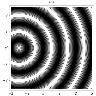
Figure 2: Invisibility device. The device transforms waves emitted in physical space as if they propagate through empty space in transformed coordinates. (a) Transformed space. The figure shows the propagation of a spherical wave emitted at the point $(-1.5,0,0)$. (b) Physical space. The invisibility device turns the wave of figure (a) into physical space by the coordinate transformation illustrated in Fig. 1. The cloaking layer with radii $R_{1}=0.5$ and $R_{2}=1.0$ deforms electromagnetic waves such that they propagate around the invisible region and leave without carrying any trace of the interior of the device.

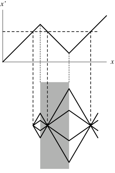
Figure 3: Perfect lens. Negatively refracting perfect lenses employ transformation media. The top figure illustrates the coordinate transformation (17) from the physical $x$ axis to $x^{\prime}$, the lower figure shows the corresponding device. The inverse transformation from $x^{\prime}$ to $x$ is either triple or single-valued. The triple-valued segment on the physical $x$ axis corresponds to the focal region of the lens: any source point has two images, one inside the lens and one on the other side. Since the device facilitates an exact coordinate transformation, the images are perfect with a resolution below the normal diffraction limit [11]: the lens is perfect [7]. In the device, the transformation changes right-handed into left-handed coordinates. Consequently, the medium employed here is left-handed, with negative refraction [8].

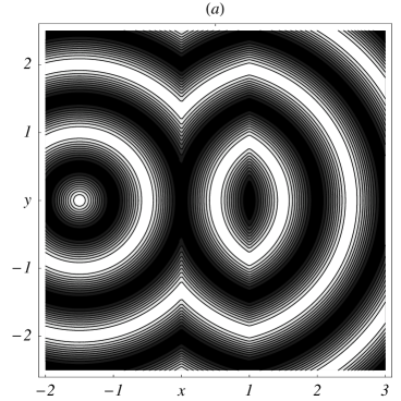
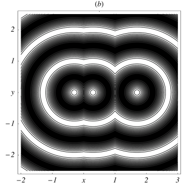
Figure 4: Propagation of electromagnetic waves in a perfect lens. The lens facilitates the coordinate transformation shown in Fig. 3. Spherical waves in electromagnetic space are transformed into physical space. (a) The wave of Fig. 2 (a) is emitted outside the imaging range of the lens. The wave is transformed by the lens, but the device is not sufficiently thick to form an image. (b) A wave is emitted inside the imaging range, creating two images of the emission point, one inside the device and one outside, corresponding to the image points of Fig. 3.

Suppose a transformation medium acts on the electromagnetic field in the vacuum state. Although the medium appears to merely transform one nothing into another, it may cause surprising physical phenomena: for example [12], the Casimir force [13] may become repulsive in left-handed transformation media [2, 8], possibly even to the extent of levitating ultra-light metal foils. This effect [12] follows from the quantum optics of spatial transformation media set out in this paper.

The quantum theory of light in isotropic media has been the subject of an extensive literature [9, 14], left-handed media have been considered [15] with respect to their modification of the spontaneous emission of atoms, but not transformation media in general. Such media are bi-anisotropic: both the electric permittivity $\varepsilon$ and the magnetic permeability $\mu$ are real symmetric matrices that may spatially vary. Following Knöll, Vogel, and Welsch [16] and Glauber and Lewenstein [17], we develop a concise quantum theory of light in non-dispersive bi-anisotropic media. Then we show how the quantum optics of transformation media emerges from this theory. Although most transformation media are strongly dispersive, our simple non-dispersive theory is capable to describe the essence of some unusual quantum effects, for example quantum levitation due to repulsive Casimir forces [12].

2 Bi-anisotropic media

Consider quantum electromagnetism in non-dispersive media, i.e. in frequency ranges where dispersion and absorption are negligible. The media are described by the constitutive equations in SI units

$$\widehat{\mathbf{D}}=\varepsilon_{0}\varepsilon\widehat{\mathbf{E}}\,,\quad\widehat{\mathbf{B}}=\frac{\mu}{\varepsilon_{0}c^{2}}\,\widehat{\mathbf{H}}\,.$$ (1)

Throughout this paper we denote vectors in bold type. The Hamiltonian, the quantum operator of the electromagnetic energy in such media, is [18]

$$\hat{H}=\frac{1}{2}\int\left(\widehat{\mathbf{E}}\cdot\widehat{\mathbf{D}}+\widehat{\mathbf{B}}\cdot\widehat{\mathbf{H}}\right)\mathrm{d}V\,.$$ (2)

Note that the Hamiltonian describes the energy of both the electromagnetic field and the medium. In the absence of any external charges and currents [16, 17], we employ the operator $\widehat{\mathbf{A}}$ of the vector potential in order to describe the electromagnetic field as

$$\widehat{\mathbf{E}}=-\frac{\partial\widehat{\mathbf{A}}}{\partial t}\,,\quad\widehat{\mathbf{B}}=\nabla\times\widehat{\mathbf{A}}\,.$$ (3)

In Coulomb gauge [17, 19],

$$\nabla\cdot\varepsilon\widehat{\mathbf{A}}=0\,,$$ (4)

Maxwell’s equations are naturally satisfied, except

$$\nabla\times\widehat{\mathbf{H}}=\frac{\partial\widehat{\mathbf{D}}}{\partial t}\,.$$ (5)

The quantum field $\widehat{\mathbf{A}}$ shall obey both the Coulomb and Maxwell equations (4) and (5). Additionally, we postulate the fundamental equal-time commutation relation

$$\big{[}\widehat{\mathbf{D}}(\mathbf{r}_{1},t),\widehat{\mathbf{A}}(\mathbf{r}_{2},t)\big{]}=i\hbar\,\delta^{T}(\mathbf{r}_{1},\mathbf{r}_{2})$$ (6)

where $\delta^{T}(\mathbf{r}_{1},\mathbf{r}_{2})$ denotes the transversal delta function [17, 19] that is consistent with the Coulomb gauge (4). One may motivate the commutation relation (6) by requiring that both the relation $\widehat{\mathbf{E}}=-\partial\widehat{\mathbf{A}}/{\partial t}$ and the Maxwell equation (5) should follow from the Hamiltonian (2) in the form

$$\hat{H}=\frac{1}{2\varepsilon_{0}}\int\left(\widehat{\mathbf{D}}\,\varepsilon^{-1}\widehat{\mathbf{D}}+\varepsilon_{0}^{2}c^{2}\widehat{\mathbf{B}}\,\mu^{-1}\widehat{\mathbf{B}}\right)\mathrm{d}V$$ (7)

with $\widehat{\mathbf{B}}=\nabla\times\widehat{\mathbf{A}}$. Alternatively, the canonical quantization procedure [19] of classical electromagnetism in media [18] leads to the commutation relation (6). Due to the interaction of the field with the dipoles of the medium, the canonical field momentum depends on the medium; and so relation (6) connects the vector potential, a pure field quantity, with the dielectric displacement that describes both the field and the medium.

Since the Coulomb-Maxwell equations (4) and (5) are linear, we can expand $\widehat{\mathbf{A}}$ in terms of a complete set of modes $\mathbf{A}_{k}(\mathbf{r},t)$ that obey the classical field equations (4) and (5),

$$\widehat{\mathbf{A}}=\sum_{k}\left(\mathbf{A}_{k}\hat{a}_{k}+\mathbf{A}_{k}^{*}\hat{a}_{k}^{\dagger}\right)\,.$$ (8)

The mode functions $\mathbf{A}_{k}(\mathbf{r},t)$ describe the classical aspects of the electromagnetic field, for example electromagnetic wave packets propagating in space and time through the medium, whereas the operators $\hat{a}_{k}$ and $\hat{a}_{k}^{\dagger}$ are constant and describe the quantum excitations of the field, the photons. In order to discriminate between photons with different quantum numbers $k$, we employ the scalar product

$$\left(\mathbf{A}_{1},\mathbf{A}_{2}\right)\equiv-\frac{i}{\hbar}\int\left(\mathbf{A}_{1}^{*}\cdot\mathbf{D}_{2}-\mathbf{A}_{2}\cdot\mathbf{D}_{1}^{*}\right)\mathrm{d}V$$ (9)

where the $\mathbf{D}$ are connected to the $\mathbf{A}$ by the classical constitutive equations (1) and (3). The modes may evolve in time, but their scalar product remains conserved, because

$$\frac{\mathrm{d}\left(\mathbf{A}_{1},\mathbf{A}_{2}\right)}{\mathrm{d}t} = \frac{i}{\hbar}\int\Bigg{(}\mathbf{E}_{1}^{*}\cdot\mathbf{D}_{2}-\mathbf{E}_{2}\cdot\mathbf{D}_{1}^{*}-\mathbf{A}_{1}^{*}\cdot\frac{\partial\mathbf{D}_{2}}{\partial t}+\mathbf{A}_{2}\cdot\frac{\partial\mathbf{D}_{1}^{*}}{\partial t}\Bigg{)}\,\mathrm{d}V\,,$$

$$\mathbf{A}\cdot\frac{\partial\mathbf{D}}{\partial t} = \mathbf{A}\cdot(\nabla\times\mathbf{H})=-\nabla\cdot(\mathbf{A}\times\mathbf{H})+\mathbf{B}\cdot\mathbf{H}\,,$$ (10)

together with the matrix symmetry of $\varepsilon$ and $\mu$ in the constitutive equations (1), implies that the time derivative of $\left(\mathbf{A}_{1},\mathbf{A}_{2}\right)$ vanishes. We require

$$\left(\mathbf{A}_{k},\mathbf{A}_{k^{\prime}}\right)=\delta_{kk^{\prime}}\,,\quad\left(\mathbf{A}_{k}^{*},\mathbf{A}_{k^{\prime}}\right)=0\,,$$ (11)

use these orthonormality conditions to extract the mode operators from the expansion (8) as $\hat{a}_{k}=\big{(}\mathbf{A}_{k},\widehat{\mathbf{A}}\big{)}$ and $\hat{a}_{k}^{\dagger}=-\big{(}\mathbf{A}_{k}^{*},\widehat{\mathbf{A}}\big{)}$, and obtain from the fundamental field commutator (6) the Bose commutation relations

$$[\hat{a}_{k},\hat{a}_{k^{\prime}}^{\dagger}]=\delta_{kk^{\prime}}\,,\quad[\hat{a}_{k},\hat{a}_{k^{\prime}}]=0\,.$$ (12)

Like light in free space, light in a bi-anisotropic medium consists of electromagnetic oscillators with the annihilation and creation operators $\hat{a}_{k}$ and $\hat{a}_{k}^{\dagger}$. The photons are the quanta of the independent degrees of freedom of the electromagnetic field. As we have seen, their fundamental character is not influenced by the medium. However, the physics of the medium is important in identifying the photons via the scalar product (9), and the mode functions $\mathbf{A}_{k}(\mathbf{r},t)$ naturally depend on the medium.

For stationary modes with frequencies $\omega_{k}$ the Hamiltonian (2) appears as

$$\hat{H}=\frac{1}{2}\int\left(\widehat{\mathbf{E}}\cdot\widehat{\mathbf{D}}+\widehat{\mathbf{A}}\cdot\frac{\partial\widehat{\mathbf{D}}}{\partial t}\right)\mathrm{d}V=\sum_{k}\hbar\omega_{k}\left(\hat{a}_{k}^{\dagger}\hat{a}_{k}+\frac{1}{2}\right)\,,$$ (13)

a sum of harmonic-oscillator energies, including the zero-point energies $\hbar\omega_{k}/2$. The frequencies $\omega_{k}$ depend on the medium and the boundary conditions. The total zero-point energy $E_{0}$ is infinite, but the derivative of $E_{0}$ with respect to the boundaries is finite [13]: giving rise to the Casimir force.

3 Spatial transformation media

Suppose that the electric permittivity $\varepsilon$ and the magnetic permeability $\mu$ in Cartesian coordinates $x^{i}$ are given by the matrices

$$\varepsilon=\frac{JJ^{T}}{\mathrm{det}J}\,\varepsilon^{\prime}\,,\quad\mu=\frac{JJ^{T}}{\mathrm{det}J}\,\mu^{\prime}\,,\quad J^{i}_{j}=\frac{\partial x^{i}}{\partial x^{\prime j}}\,.$$ (14)

The coordinates $x^{i}$ and the scalars $\varepsilon^{\prime}$ and $\mu^{\prime}$ are functions of some transformed coordinates $x^{\prime j}$. In regions where the coordinates agree, $J$ reduces to the unity matrix; and so $\varepsilon^{\prime}$ and $\mu^{\prime}$ directly describe the dielectric properties of the medium here. In the following we show that the quantum optics of the general medium (14) in physical space is mapped, in the primed coordinates, to quantum electrodynamics in the presence of a dielectric with $\varepsilon^{\prime}$ and $\mu^{\prime}$, for the transformed vector potential

$$\widehat{\mathbf{A}}^{\prime}=J\widehat{\mathbf{A}}\quad\mbox{or, equivalently,}\quad\hat{A}_{i}^{\prime}=\sum_{j}J^{j}_{i}\hat{A}_{j}\,.$$ (15)

First we write $\varepsilon$ and $\mu^{-1}$ in component representation,

$$\varepsilon = \pm\sqrt{\gamma}\,\gamma^{ij}\,\varepsilon^{\prime}\,,\quad\mu^{-1}=\pm\frac{\gamma_{ij}}{\sqrt{\gamma}\,\mu^{\prime}}\,,\quad\gamma=\mathrm{det}(\gamma_{ij})\,,$$

$$\gamma^{ij} = \sum_{l}\frac{\partial x^{i}}{\partial x^{\prime l}}\frac{\partial x^{j}}{\partial x^{\prime l}}\,,\quad\gamma_{ij}=\sum_{l}\frac{\partial x^{\prime l}}{\partial x^{i}}\frac{\partial x^{\prime l}}{\partial x^{j}}\,.$$ (16)

These are the constitutive equations of spatial transformation media [2] expressed in terms of the spatial metric $\gamma_{ij}$, the matrix inverse of $\gamma^{ij}$. The $\pm$ sign distinguishes between right and left-handed coordinate systems where the Jacobian $\mathrm{det}J$ is positive or negative, respectively. Left-handed systems thus correspond to left-handed materials [8] where the eigenvalues of $\varepsilon$ and $\mu$ are negative [2]. Consider for example the transformation [2]

$$x^{\prime}=\left\{\begin{array}[]{rcl}x&\mbox{for}&x<0\\ -x&\mbox{for}&0\leq x\leq b\\ x-2b&\mbox{for}&x>b\end{array}\right.$$ (17)

illustrated in Fig. 3. In the region $0\leq x\leq b$, Eq. (17) transforms a right-handed Cartesian coordinate system into a left-handed one. We see from Eq. (14) that the transformation (17) is performed by a left-handed medium with $\varepsilon=\mu=-1$ inside the slab and $\varepsilon=\mu=1$ outside [2].

Quantum electrodynamics in bi-anisotropic media is characterized by the vector potential $\widehat{\mathbf{A}}$ subject to both the Coulomb gauge (4) and the Maxwell equation (5). We express the Coulomb-gauge condition as

$$0=\pm\frac{\nabla\cdot\varepsilon\widehat{\mathbf{A}}}{\sqrt{\gamma}}=\frac{1}{\sqrt{\gamma}}\sum_{ij}\frac{\partial\sqrt{\gamma}\,\gamma^{ij}\varepsilon^{\prime}\hat{A}_{j}}{\partial x^{i}}\,,$$ (18)

which is the covariant form of the 3D divergence [20] if we interpret $\gamma_{ij}$ as the metric tensor of physical space: the physical Cartesian coordinates $x^{i}$ appear as the back-transformed primed coordinates $x^{\prime j}$ of a space where the metric tensor $\gamma_{ij}^{\prime}$ is the unity matrix; the transformed space is flat. Consequently, we obtain here

$$0=\nabla^{\prime}\cdot\varepsilon^{\prime}\widehat{\mathbf{A}}^{\prime}\,.$$ (19)

Now we turn to the Maxwell equation (5). We apply the constitutive equation (1) for $\widehat{\mathbf{D}}$ with the electric permittivity (16) and write the electric field in terms (3) of the vector potential,

$$\varepsilon_{0}\sum_{j}\gamma^{ij}\varepsilon^{\prime}\,\frac{\partial^{2}\hat{A}_{j}}{\partial t^{2}}=\mp\frac{(\nabla\times\widehat{\mathbf{H}})^{i}}{\sqrt{\gamma}}\,.$$ (20)

Then we express the components of the curl in terms of the 3D Levi-Civita tensor $\epsilon^{ijl}$ for the spatial geometry characterized by the metric tensor $\gamma_{ij}$ [20],

$$\pm\frac{(\nabla\times\widehat{\mathbf{H}})^{i}}{\sqrt{\gamma}}=\sum_{jl}\epsilon^{ijl}\,\frac{\partial\hat{H}_{l}}{\partial x^{j}}\,.$$ (21)

We invert the constitutive equations (1) for $\widehat{\mathbf{B}}$ using the representation (16) of $\mu^{-1}$ in terms of the metric tensor,

$$\hat{H}_{i}=\frac{\varepsilon_{0}c^{2}}{\mu^{\prime}}\sum_{j}\gamma_{ij}\left(\pm\frac{\hat{B}^{j}}{\sqrt{\gamma}}\right)\,,$$ (22)

apply the matrix $\gamma^{ij}$ to $\widehat{\mathbf{H}}$ and, like in Eq. (21), represent $\widehat{\mathbf{B}}$ as the curl of $\widehat{\mathbf{A}}$ in covariant form [20],

$$\sum_{j}\gamma^{ij}\hat{H}_{j}=\frac{\varepsilon_{0}c^{2}}{\mu^{\prime}}\sum_{jl}\epsilon^{ijl}\,\frac{\partial\hat{A}_{l}}{\partial x^{j}}\,.$$ (23)

Equations (20), (21), and (23) combined are covariant, such that we obtain in transformed space

$$\frac{1}{\varepsilon^{\prime}}\nabla^{\prime}\times\frac{1}{\mu^{\prime}}\nabla^{\prime}\times\widehat{\mathbf{A}}^{\prime}=-\frac{1}{c^{2}}\,\frac{\partial^{2}\widehat{\mathbf{A}}^{\prime}}{\partial t^{2}}\,.$$ (24)

Consequently, the Coulomb-Maxwell equations (19) and (24) for the transformed quantum field $\widehat{\mathbf{A}}^{\prime}$ are the ones of flat space filled with a medium of permittivity $\varepsilon^{\prime}$ and permeability $\mu^{\prime}$. All the other building blocks of the quantum theory of light in transformation media, the Hamiltonian (2), the field commutator (6), and the scalar product (9), are naturally covariant and are therefore mapped to flat space, too.

4 Conclusions

We developed the quantum theory of light in dispersion-less bi-anisotropic media. The theory shows how transformation media [1, 2] map quantum optics in physical space to the quantum electromagnetism in flat space. Note that even in the extreme case when the electromagnetic field is in the vacuum state, when literally nothing appears to be mapped to nothing, transformation media may cause surprising physical effects: the Casimir force in left-handed materials [8] may be repulsive [12].

We thank J. W. Allen, M. Killi, J. B. Pendry and S. Scheel for their comments and the Leverhulme Trust for financial support.

References

• [1] J. B. Pendry, D. Schurig, and D. R. Smith, Science 312, 1780 (2006); D. Schurig, J. B. Pendry, and D. R. Smith, Opt. Express 14, 9794 (2006).
• [2] U. Leonhardt and T. G. Philbin, New J. Phys. 8, 247 (2006).
• [3] D. Schurig et al., Science 314, 977 (2006).
• [4] U. Leonhardt, Science 312, 1777 (2006); New J. Phys. 8, 118 (2006).
• [5] A. Hendi, J. Henn, and U. Leonhardt, Phys. Rev. Lett. 97, 073902 (2006).
• [6] W. Cai et al. Nature Photonics 1, 224 (2007); U. Leonhardt, ibid. 1 207 (2007).
• [7] J. B. Pendry, Phys. Rev. Lett. 85, 3966 (2000).
• [8] V. Veselago et al., J. Comp. Theor. Nanoscience 3, 189 (2006).
• [9] U. Leonhardt, Rep. Prog. Phys. 66, 1207 (2003).
• [10] R. SchΓΌtzhold and W. G. Unruh, Phys. Rev. Lett. 95, 031301 (2005).
• [11] M. Born and E. Wolf, Principles of Optics (Cambridge University Press, Cambridge, 1999).
• [12] U. Leonhardt and T. G. Philbin, arxiv:quant-ph/0608115; New. J. Phys. (in press).
• [13] P. W. Milonni, The Quantum Vacuum (Academic, London, 1994); S. K. Lamoreaux, Am. J. Phys. 67, 850 (1999); Rep. Prog. Phys. 68, 201 (2005); M. Bordag, U. Mohideen, and V. M. Mostepanenko, Phys. Rep, 353, 1 (2001).
• [14] See e.g. L. KnΓΆll, S. Scheel, and D.-G.Welsch, QED in dispersing and absorbing media, in Coherence and Statistics of Photons and Atoms ed. by J. Perina (Wiley, New York, 2001); A. Luks and V. Perinova, Prog. Opt. 43, 295 (2002); S. Y. Buhmann and D.-G. Welsch, arXiv:quant-ph/0608118, Prog. Quant. Electron. (in press).
• [15] V. V. Klimov, Opt. Commun. 211, 183 (2002); Ho Trung Dung et al., Phys. Rev. A 68, 043816 (2003); J. KΓ€stel and M. Fleischhauer, ibid. 71, 011804 (2005).
• [16] L. KnΓΆll, W. Vogel, and D. -G. Welsch, Phys. Rev. A 36, 3803 (1987).
• [17] R. J. Glauber and M. Lewenstein, Phys. Rev. A 43, 467 (1991).
• [18] L. D. Landau and E. M. Lifshitz, Electrodynamics of Continuous Media (Butterworth-Heinemann, Oxford, 1993).
• [19] S. Weinberg, The Quantum Theory of Fields (Cambridge University Press, Cambridge, 1999), Volume I.
• [20] Ch. W. Misner, K. S. Thorne, and J. A. Wheeler, Gravitation (Freeman, New York, 1999).