Harmonic entanglement in a degenerate parametric down conversion

Abstract

We study the harmonic entanglement and squeezing in a two-mode radiation produced in a degenerate parametric down conversion process coupled to a two-mode vacuum reservoir employing the linearization procedure. It is found that there is a quadrature entanglement between the harmonically related fundamental and second-harmonic modes and the superimposed radiation exhibits a significant two-mode squeezing. The entanglement exits even when there is no two-mode squeezing, since the correlation leading to these phenomena are essentially different. In addition, the more the external coherent light is down converted, the more stronger the entanglement and mean photon number of the two-mode radiation would be which is not generally true for squeezing.

I INTRODUCTION

Optical degenerate parametric down convrsion is one of the second-order nonlinear processes in which a pump photon of frequency $2\omega$ is down converted into a pair of signal photons each of frequency $\omega$. Due to the inherent two-photon nature of the interaction, the parametric oscillator or amplifier is one of the most interesting and well studied devices in the nonlinear quantum optics 1 ; 2 ; 3 ; 4 ; 5 ; 6 ; 7 ; sint071 ; sint072 ; sintq . It is found to be a good source of light with nonclassical features. The quantum optical properties are significantly degraded by the leakage through the mirrors and amplification of the quantum fluctuations in the cavity. However, if the ordinary vacuum is replaced by a squeezed vacuum reservoir, the nonclassical properties can be enhanced 6 ; 7 ; 8 provided that the reservoir is squeezed in the right quadrature, since the fluctuations entering the cavity is biased. Moreover, when a nonlinear crystal is shined with an external radiation of frequency $2\omega$ only some part of this radiation is down converted into a pair of photons sint071 . As a result, the cavity contains the down converted and unchanged radiations. Although a considerable attention has been given to a single-mode squeezed radiation previously, most recently it is envisioned that a degenerate parametric oscillator can be a source of a two-mode light with nonclassical properties characterized by a strong correlation between the states of each mode separately as well as the superimposed state formed by the two radiations sint072 .

Currently, generation of macroscopic entangled states is receiving attention in connection with their potential in the quantum information and measurement theories 9 ; 10 . At microscopic level nonclassical correlations and entanglement arise due to the down conversion of a single high frequency photon into a pair of correlated lower frequency photons. The generation of the entangled beams in the nondegenerate parametric down conversion was predicted by Reid and Drummond 11 ; 12 ; 13 . Studies have also shown the existence of the correlation between the fundamental and second-harmonic modes 14 including entanglement in the second-harmonic generation 15 . In this respect, Lim and Saffman 16 analyzed the production of two beams with nonclassical intensity correlations and quadrature entanglement in the dual-ported reservoir of the second-harmonic generation and found that the harmonic output exhibits strong quantum correlations. In connection to this, Grosse et al. 17 predicted a perfect entanglement between the fundamental and second-harmonic modes in the pump depleted nondegenerate parametric amplification and defined such an entanglement between harmonically related fields as harmonic entanglement.

Einstein-Podolsky-Rosen (EPR) presented in 1935 18 their famous argument, which on the basis of the local realism claimed that an observation of perfectly correlated positions and momenta would imply the incompleteness of the quantum theory. The essential step in realizing the EPR-type entanglement is then to introduce correlated states of at least two particles that persist even when the particles are spatially separated. As thoroughly discussed by Dechoum et al. 19 without having to construct an experimentally impossible states with perfect correlation, as in the original paper, it is possible to demonstrate this type of correlation using the inferred Heisenberg principle. In this regard, a direct and experimentally feasible qualitative criterion for such a correlation of continuous variables was first proposed by Reid 12 via quadrature phase amplitude, applying a nondegenerate parametric amplification, which is closely related to the original version. In addition, making use of the quadrature variables Lodahl lod showed the existence of EPR-type correlations in the second-harmonic generation. Most recently, Olsen 15 has considered a travelling-wave second-harmonic generation and predicted that this quantum system can be employed in the experimental demonstration of entanglement with continuous variables. It then appears natural to ask whether the strong correlation between the fundamental and second-harmonic modes of the degenerate parametric oscillator associated with the down conversion also leads to entanglement or not? The main task of this communication is, therefore, devoted to answer this question.

In this paper, the nonclassical properties of the two-mode cavity radiation of the driven degenerate parametric oscillator coupled to a two-mode vacuum reservoir applying the linearization procedure in which the quantum properties of the system in time are taken to vary slightly around the steady state mean values would be analyzed. As discussed by Gilles et al. 21 , this approximation remains valid as long as the quantum fluctuations are much smaller than the classical mean values which is the essence of a weaker coupling of the radiation with the oscillator that corresponds to small quadrature noise. We also consider the semiclassical approximation whereby the two modes are assumed to be uncorrelated at steady state. As recently reported by Chaturvedi et al. 22 , the semiclassical theory is found to work surprisingly well in the threshold region. We hence study the harmonic entanglement and its relation with the squeezing near threshold, since the relation between the two is an interesting issue by its own right prl93063601 ; prl95120502 . Moreover, we investigate the efficiency with which a nonlinear crystal down convert the light falling on it and the association of the down conversion with the entanglement and squeezing. We also calculate the mean photon number to see how intense the generated light could be.

II Quantum Langevin Equations

Interaction of an external coherent radiation with a nonlinear crystal responsible for a degenerate parametric oscillation placed in a resonant cavity can be described in the rotating-wave approximation and in interaction picture by the Hamiltonian of the form

$$\hat{H}_{I}={i\lambda\over 2}\left[\hat{a}^{\dagger^{2}}\hat{b}-\hat{a}^{2}\hat{b}^{\dagger}\right]+i\varepsilon\left[\hat{b}^{\dagger}-\hat{b}\right],$$ (1)

where $\varepsilon$ is proportional to the amplitude of the coherent input, $\lambda$ is the measure of the coupling of a nonlinear crystal with the external coherent radiation, $\hat{a}$ and $\hat{b}$ are the time-independent annihilation operators for the fundamental (subharmonic) and pumping (second-harmonic) modes, and $\lambda$ and $\varepsilon$ are chosen to be real-positive constants. In view of the fact that $\hat{a}$ and $\hat{b}$ are mutually commuting operators, the pertinent quantum Langevin equations are found to be

$${d\hat{a}\over dt}=\lambda\hat{a}^{\dagger}\hat{b}-{\kappa\over 2}\hat{a}+\hat{F}_{a}(t),$$ (2)

$${d\hat{b}\over dt}=-{\lambda\over 2}\hat{a}^{2}-{\kappa\over 2}\hat{b}+\varepsilon+\hat{F}_{b}(t),$$ (3)

where $\kappa$ is the cavity damping constant chosen to be the same for both modes and $\hat{F}_{i}(t)$, with $i=a,b$, are the Langevin noise operators satisfying, for a two-mode vacuum reservoir, the correlation functions:

$$\langle\hat{F}_{i}(t)\rangle=0,$$ (4)

$$\langle\hat{F}_{i}^{\dagger}(t)\hat{F}_{j}(t^{\prime})\rangle=\langle\hat{F}_{i}^{\dagger}(t)\hat{F}_{j}^{\dagger}(t^{\prime})\rangle=\langle\hat{F}_{i}(t)\hat{F}_{j}(t^{\prime})\rangle=0,$$ (5)

$$\langle\hat{F}_{i}(t)\hat{F}_{i}^{\dagger}(t^{\prime})\rangle=\kappa\delta(t-t^{\prime}),$$ (6)

$$\langle\hat{F}_{i}(t)\hat{F}^{\dagger}_{j}(t^{\prime})\rangle_{i\neq j}=0.$$ (7)

We notice that Eqs. (2) and (3) are nonlinear coupled differential equations that can be solved employing the linearization procedure. In this approach, we first take

$$\hat{a}(t)=\alpha+\hat{A}(t),$$ (8)

$$\hat{b}(t)=\beta+\hat{B}(t),$$ (9)

where $\hat{A}(t)$ and $\hat{B}(t)$ are very small variations about the mean values at steady state, and we define   $\alpha=\langle\hat{a}(t)\rangle_{ss}$ and $\beta=\langle\hat{b}(t)\rangle_{ss}$. This approximation remains valid as long as the quantum fluctuations about the mean values are much smaller than the classical mean values, which implies that the quantum noise during the interaction is quite small. Upon taking the statistical average of Eqs. (2) and (3) and then using the semiclassical approximation, whereby at steady state the modes are assumed to be uncorrelated, $\langle\hat{a}^{\dagger}(t)\hat{b}(t)\rangle_{ss}=\langle\hat{a}^{\dagger}(t)\rangle_{ss}\langle\hat{b}(t)\rangle_{ss},$ and classical decorrelation that operators are assumed to be factorized, $\langle\hat{a}^{2}(t)\rangle_{ss}=\langle\hat{a}(t)\rangle^{2}_{ss},$ we obtain

$$\lambda\alpha^{*}\beta-{\kappa\over 2}\alpha=0,$$ (10)

$$\lambda\alpha^{2}+\kappa\beta=2\varepsilon.$$ (11)

We realize that the semiclassical assumption is found to work for weak nonlinearity or weak coupling between the external radiation and nonlinear crystal where the mean photon number at threshold is very large.

Now with the aid of Eqs. (2), (3), (8), (9), (10), (11), and the fact that $\hat{A}$ and $\hat{B}$ are small perturbations, it is possible to verify that

$${d\hat{A}(t)\over dt}=\varepsilon_{1}^{*}\hat{B}(t)+\varepsilon_{2}\hat{A}^{\dagger}(t)-{\kappa\over 2}\hat{A}(t)+\hat{F}_{a}(t),$$ (12)

$${d\hat{B}(t)\over dt}=-\varepsilon_{1}\hat{A}(t)-{\kappa\over 2}\hat{B}(t)+\hat{F}_{b}(t),$$ (13)

where we set $\varepsilon_{1}^{*}=\lambda\alpha^{*}$ and $\varepsilon_{2}=\lambda\beta$. Multiplication of Eq. (10) by $\alpha$ suggests that the phase of $\beta$ is the same as that of $\alpha^{2}$. This is consistent with Eq. (11) if both $\alpha$ and $\beta$ are real, which implies that $\varepsilon_{1}$ and $\varepsilon_{2}$ are also real. It then follows from Eqs. (10) and (11) that

$$\varepsilon_{1}=\pm\sqrt{2\lambda\varepsilon-\kappa\varepsilon_{2}}$$ (14)

and $\varepsilon_{2}=\kappa/2$ for $\varepsilon_{1}\neq 0$. We notice that there are two possible values for the fundamental amplitude and hence the system may be in a transient superimposed state of these amplitudes prior to detection 10 . Moreover, the solutions of these coupled differential equations are found following a straight forward algebra to be

$$\hat{A}(t) =a_{1}(t)+\big{[}a_{3}(t)+pa_{4}(t)\big{]}\hat{A}(0)+\big{[}a_{5}(t)+pa_{6}(t)\big{]}$$

$$\times\hat{A}^{\dagger}(0)+qa_{6}(t)\hat{B}(0)+qa_{4}(t)\hat{B}^{\dagger}(0)+\hat{f}(t),$$ (15)

$$\hat{B}(t) =a_{2}(t)+\big{[}a_{3}(t)-pa_{4}(t)\big{]}\hat{B}(0)+\big{[}a_{5}(t)-pa_{6}(t)\big{]}$$

$$\times\hat{B}^{\dagger}(0)-qa_{6}(t)\hat{A}(0)-qa_{4}(t)\hat{A}^{\dagger}(0)+\hat{g}(t),$$ (16)

where

$$\hat{f}(t) =\int_{0}^{t}\big{[}\big{(}a_{3}(t-t^{\prime})+pa_{4}(t-t^{\prime})\big{)}\hat{F}_{a}(t^{\prime})$$

$$+\big{(}a_{5}(t-t^{\prime})+pa_{6}(t-t^{\prime})\big{)}\hat{F}^{\dagger}_{a}(t^{\prime})$$

$$+qa_{6}(t-t^{\prime})\hat{F}_{b}(t^{\prime})+qa_{4}(t-t^{\prime})\hat{F}^{\dagger}_{b}(t^{\prime})\big{]}dt^{\prime},$$ (17)

$$\hat{g}(t) =\int_{0}^{t}\big{[}\big{(}a_{3}(t-t^{\prime})-pa_{4}(t-t^{\prime})\big{)}\hat{F}_{b}(t^{\prime})$$

$$+\big{(}a_{5}(t-t^{\prime})-pa_{6}(t-t^{\prime})\big{)}\hat{F}^{\dagger}_{b}(t^{\prime})$$

$$-qa_{6}(t-t^{\prime})\hat{F}_{a}(t^{\prime})-qa_{4}(t-t^{\prime})\hat{F}^{\dagger}_{a}(t^{\prime})\big{]}dt^{\prime},$$ (18)

in which

$$p={\varepsilon_{2}\over\sqrt{\varepsilon_{2}^{2}-4\varepsilon_{1}^{2}}},$$ (19)

$$q={2\varepsilon_{1}\over\sqrt{\varepsilon_{2}^{2}-4\varepsilon_{1}^{2}}},$$ (20)

$$a_{1}(t) =-{e^{-{(\kappa-\varepsilon_{2})t\over 2}}\over\lambda}\left[\varepsilon_{1}\cosh\left({t\sqrt{\varepsilon_{2}^{2}-4\varepsilon_{1}^{2}}\over 2}\right)\right.$$

$$\left.+\big{(}\varepsilon_{1}p+\varepsilon_{2}q\big{)}\sinh\left({t\sqrt{\varepsilon_{2}^{2}-4\varepsilon_{1}^{2}}\over 2}\right)\right],$$ (21)

$$a_{2}(t) =-{e^{-{(\kappa-\varepsilon_{2})t\over 2}}\over\lambda}\left[\big{(}\varepsilon_{1}q+\varepsilon_{2}p\big{)}\sinh\left({t\sqrt{\varepsilon_{2}^{2}-4\varepsilon_{1}^{2}}\over 2}\right)\right.$$

$$\left.-\varepsilon_{2}\cosh\left({t\sqrt{\varepsilon_{2}^{2}-4\varepsilon_{1}^{2}}\over 2}\right)\right],$$ (22)

$$a_{3}(t)=e^{-{\kappa t\over 2}}\cosh\left({\varepsilon_{2}t\over 2}\right)\cosh\left({t\sqrt{\varepsilon_{2}^{2}-4\varepsilon_{1}^{2}}\over 2}\right),$$ (23)

$$a_{4}(t)=e^{-{\kappa t\over 2}}\sinh\left({\varepsilon_{2}t\over 2}\right)\sinh\left({t\sqrt{\varepsilon_{2}^{2}-4\varepsilon_{1}^{2}}\over 2}\right),$$ (24)

$$a_{5}(t)=e^{-{\kappa t\over 2}}\sinh\left({\varepsilon_{2}t\over 2}\right)\cosh\left({t\sqrt{\varepsilon_{2}^{2}-4\varepsilon_{1}^{2}}\over 2}\right),$$ (25)

$$a_{6}(t)=e^{-{\kappa t\over 2}}\cosh\left({\varepsilon_{2}t\over 2}\right)\sinh\left({t\sqrt{\varepsilon_{2}^{2}-4\varepsilon_{1}^{2}}\over 2}\right).$$ (26)

It may worth to mention that Eqs. (II) and (II) are applied to calculate various quantities of interest. We also observe that the condition for $\varepsilon_{1}$ to be real requires that $2\lambda\varepsilon\geq\kappa\varepsilon_{2}$. We, therefore, denote the case for which $2\lambda\varepsilon=\kappa\varepsilon_{2}$ that corresponds to $\varepsilon_{1}=0$ as a threshold condition.

III Quadrature Entanglement

In this section, we seek to study the entanglement of the fundamental and second-harmonic modes in the cavity. It is a well-established fact that a quantum system is said to be entangled, if it is not separable. That is, if the density operator for the combined state cannot be expressed as a combination of the product density operators of the constituents,

$$\hat{\rho}\neq\sum_{j}\hat{\rho}_{j}^{(1)}\bigotimes\hat{\rho}_{j}^{(2)}.$$ (27)

On the other hand, entangled continuous variable state can be expressed as a co-eigenstate of a pair of EPR-type operators such as $\hat{X}_{a}-\hat{X}_{b}$ and $\hat{P}_{a}+\hat{P}_{b}$ pra74 . The total variance of these two operators reduces to zero for maximally entangled continuous variable states. Nonetheless, according to the criterion set by Duan et al. duan quantum states of the system are entangled, provided that the sum of the variances of a pair of EPR-like operators

$$\hat{u}=\hat{X}_{a}-\hat{X}_{b},$$ (28)

$$\hat{v}=\hat{P}_{a}+\hat{P}_{b},$$ (29)

where $\hat{X}_{a}={1\over\sqrt{2}}\big{(}\hat{a}+\hat{a}^{\dagger}\big{)}$, $\hat{X}_{b}={1\over\sqrt{2}}\big{(}\hat{b}+\hat{b}^{\dagger}\big{)}$,
$\hat{P}_{a}={i\over\sqrt{2}}\big{(}\hat{a}^{\dagger}-\hat{a}\big{)}$, and $\hat{P}_{b}={i\over\sqrt{2}}\big{(}\hat{b}^{\dagger}-\hat{b}\big{)}$, satisfy

$$\Delta u^{2}+\Delta v^{2}<2,$$ (30)

in which

$$\Delta u^{2}+\Delta v^{2} =2\langle\hat{a}^{\dagger}\hat{a}\rangle+2\langle\hat{b}^{\dagger}\hat{b}\rangle+2\langle\hat{a}\rangle\langle\hat{b}\rangle+2\langle\hat{a}^{\dagger}\rangle\langle\hat{b}^{\dagger}\rangle$$

$$-2\langle\hat{a}\hat{b}\rangle-2\langle\hat{a}^{\dagger}\hat{b}^{\dagger}\rangle-2\langle\hat{a}^{\dagger}\rangle\langle\hat{a}\rangle-2\langle\hat{b}^{\dagger}\rangle\langle\hat{b}\rangle+2.$$ (31)

Next we determine the various correlations in Eq. (III). To this end, assuming the cavity mode to be initially in the vacuum state and using the fact that the Langevin noise forces have zero mean along with Eqs. (8), (9), (II), and (II), we get

$$\langle\hat{a}(t)\rangle=\alpha+a_{1}(t),$$ (32)

$$\langle\hat{b}(t)\rangle=\beta+a_{2}(t),$$ (33)

$$\langle\hat{a}^{\dagger}(t)\hat{a}(t)\rangle=\big{(}\alpha+a_{1}(t)\big{)}^{2}+\langle\hat{f}^{\dagger}(t)\hat{f}(t)\rangle,$$ (34)

$$\langle\hat{b}^{\dagger}(t)\hat{b}(t)\rangle=\big{(}\beta+a_{2}(t)\big{)}^{2}+\langle\hat{g}^{\dagger}(t)\hat{g}(t)\rangle,$$ (35)

$$\langle\hat{a}(t)\hat{b}(t)\rangle=(\alpha+a_{1}(t))(\beta+a_{2}(t))+\langle\hat{f}(t)\hat{g}(t)\rangle.$$ (36)

Moreover, in view of the correlations of the Langevin noise forces (5), (6), and (7), it is possible to show at steady state that

$$\langle\hat{f}^{\dagger}(t)\hat{f}(t)\rangle_{ss} ={\kappa[(1+p^{2}+q^{2})(\kappa-\varepsilon_{2})-2p\sqrt{\varepsilon_{2}^{2}-4\varepsilon_{1}^{2}}]\over 8[\kappa(\kappa-2\varepsilon_{2})+4\varepsilon_{1}^{2}]}$$

$$+{\kappa[(1+p^{2}+q^{2})(\kappa+\varepsilon_{2})+2p\sqrt{\varepsilon_{2}^{2}-4\varepsilon_{1}^{2}}]\over 8[\kappa(\kappa+2\varepsilon_{2})+4\varepsilon_{1}^{2}]}$$

$$+{\kappa^{2}(1-p^{2}-q^{2})\over 4(\kappa^{2}-\varepsilon_{2}^{2})}-{\kappa^{2}(1-p^{2}+q^{2})\over 4[\kappa^{2}-(\varepsilon_{2}^{2}-4\varepsilon_{1}^{2})]}$$

$$-{(1+p^{2}-q^{2})\over 4},$$ (37)

$$\langle\hat{g}^{\dagger}(t)\hat{g}(t)\rangle_{ss} ={\kappa[(1+p^{2}+q^{2})(\kappa-\varepsilon_{2})+2p\sqrt{\varepsilon_{2}^{2}-4\varepsilon_{1}^{2}}]\over 8[\kappa(\kappa-2\varepsilon_{2})+4\varepsilon_{1}^{2}]}$$

$$+{\kappa[(1+p^{2}+q^{2})(\kappa+\varepsilon_{2})-2p\sqrt{\varepsilon_{2}^{2}-4\varepsilon_{1}^{2}}]\over 8[\kappa(\kappa+2\varepsilon_{2})+4\varepsilon_{1}^{2}]}$$

$$+{\kappa^{2}(1-p^{2}-q^{2})\over 4(\kappa^{2}-\varepsilon_{2}^{2})}-{\kappa^{2}(1-p^{2}+q^{2})\over 4[\kappa^{2}-(\varepsilon_{2}^{2}-4\varepsilon_{1}^{2})]}$$

$$-{(1+p^{2}-q^{2})\over 4},$$ (38)

$$\langle\hat{f}(t)\hat{g}(t)\rangle_{ss} =-{\kappa pq(\kappa-\varepsilon_{2})\over 4[\kappa(\kappa-2\varepsilon_{2})+4\varepsilon_{1}^{2}]}$$

$$-{\kappa qp(\kappa+\varepsilon_{2})\over 4[\kappa(\kappa+2\varepsilon_{2})+4\varepsilon_{1}^{2}]}+{qp\kappa^{2}\over 2(\kappa^{2}-\varepsilon_{2}^{2})}$$

$$-{\kappa^{2}pq\over 2[\kappa^{2}-(\varepsilon_{2}^{2}-4\varepsilon_{1}^{2})]}+{pq\over 2}.$$ (39)

We, therefore, see with the aid of Eqs. (III), (32), (33), (34), (35), (36), (III), (III), and (III) at steady state that

$$\Delta u^{2}+\Delta v^{2} =2+{\kappa(1+p^{2}+q^{2}+2qp)(\kappa-\varepsilon_{2})\over 2[\kappa(\kappa-2\varepsilon_{2})+4\varepsilon_{1}^{2}]}$$

$$+{\kappa(1+p^{2}+q^{2}+2qp)(\kappa+\varepsilon_{2})\over 2[\kappa(\kappa+2\varepsilon_{2})+4\varepsilon_{1}^{2}]}$$

$$+{\kappa^{2}(1-p^{2}-q^{2}-2qp)\over(\kappa^{2}-\varepsilon_{2}^{2})}$$

$$-{\kappa^{2}(1-p^{2}+q^{2}-2qp)\over[\kappa^{2}-(\varepsilon_{2}^{2}-4\varepsilon_{1}^{2})]}$$

$$-(1+p^{2}-q^{2}+2qp).$$ (40)

Finally, on account of Eqs. (19), (20), and the fact that $\varepsilon_{2}=\kappa/2$ for $\varepsilon_{1}\neq 0$, we find

$$\Delta u^{2}+\Delta v^{2} ={\kappa^{3}(\kappa+4\varepsilon_{1})\over 8\varepsilon_{1}^{2}(\kappa^{2}-16\varepsilon_{1}^{2})}$$

$$+{3\kappa^{3}(\kappa+4\varepsilon_{1})\over 4(\kappa^{2}-16\varepsilon_{1}^{2})(\kappa^{2}+2\varepsilon_{1}^{2})}$$

$$-{16\varepsilon_{1}(4\varepsilon_{1}+\kappa)+24\kappa\varepsilon_{1}\over 3(\kappa^{2}-16\varepsilon_{1}^{2})}$$

$$+{16\kappa^{3}\varepsilon_{1}\over(\kappa^{2}-16\varepsilon_{1}^{2})(3\kappa^{2}+16\varepsilon_{1}^{2})}.$$ (41)

It is not difficult to observe that $\Delta u^{2}+\Delta v^{2}$ is very large when $\varepsilon_{1}=0$ and $\varepsilon_{1}=0.25\kappa$. We hence plot $\Delta u^{2}+\Delta v^{2}$ versus $\varepsilon_{1}$ for $\varepsilon_{1}>0.25\kappa$.

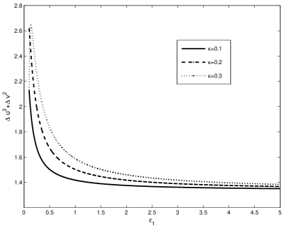
Figure 1: Plots of the sum of the variances of the EPR-type operators ($\Delta u^{2}+\Delta v^{2}$) at steady state for different values of $\kappa$.

As clearly shown in Fig. 1 the correlation between the fundamental and second-harmonic modes exhibits a quadrature entanglement except near certain value of $\varepsilon_{1}$, for example $\varepsilon_{1}=0.13$ for $\kappa=0.3$ at steady state. We also realize that entanglement does not exist near a threshold value, $\varepsilon_{1}=0$. However, entanglement exists and it decreases with damping constant in other cases for which $\varepsilon_{1}>0.25\kappa$. This is related to a well known fact that the lesser the cavity damping constant, the more the radiation stays in the cavity which in turn enhances the correlation that leads to entanglement. It is possible to observe that the dependence of the entanglement on damping through the mirrors is insignificant for larger values of $\varepsilon_{1}$. Moreover, as can easily be seen from Eq. (III) the existing entanglement is attributed to the correlation between the states of the two cavity modes. We realize that since $\varepsilon_{1}=\lambda\langle\hat{a}\rangle_{ss}$, it corresponds to the degree at which the external radiation of frequency $2\omega$ is down converted by the nonlinear crystal. Therefore, it can be inferred from Fig. 1 that the entanglement would be stronger, the more efficiently the external radiation is down converted by the crystal. This indicates that even though the down conversion process breaks the coherent external radiation into two, it is unable to destroy the coherence that is responsible for the correlation between the down converted and unchanged radiations.

IV Quadrature variances

In this section, we seek to analyze the squeezing properties of the two-mode cavity radiation which can be described by annihilation operator

$$\hat{c}={1\over\sqrt{2}}\big{(}\hat{a}+\hat{b}\big{)},$$ (42)

where $\hat{a}$ and $\hat{b}$ are the boson operators that represent the fundamental and second-harmonic modes. In view of the boson commutation relation for $\hat{a}$ and $\hat{b}$, one can easily see that $\big{[}\hat{c},\;\hat{c}^{\dagger}\big{]}=1$ and $\big{[}\hat{c},\;\hat{c}\big{]}=0$. We note that the squeezing of the two-mode cavity radiation can be studied using the quadrature operators corresponding to $\hat{c}$,

$$\hat{c}_{+}=\hat{c}^{\dagger}+\hat{c}$$ (43)

and

$$\hat{c}_{-}=i\big{(}\hat{c}^{\dagger}-\hat{c}\big{)},$$ (44)

in which the squeezing occurs when

$$\Delta c_{\pm}^{2} =1+\langle\hat{a}^{\dagger}\hat{a}\rangle+\langle\hat{b}^{\dagger}\hat{b}\rangle\pm(\langle\hat{a}\hat{b}\rangle+\langle\hat{a}^{\dagger}\hat{b}^{\dagger}\rangle)+\langle\hat{a}^{\dagger}\hat{b}\rangle$$

$$+\langle\hat{a}\hat{b}^{\dagger}\rangle\pm{1\over 2}\big{[}\langle\hat{a}^{\dagger^{2}}\rangle+\langle\hat{b}^{\dagger^{2}}\rangle+\langle\hat{a}^{2}\rangle+\langle\hat{b}^{2}\rangle+\langle\hat{a}\rangle^{2}$$

$$+\langle\hat{b}\rangle^{2}+\langle\hat{a}^{\dagger}\rangle^{2}+\langle\hat{b}^{\dagger}\rangle^{2}\big{]}\pm(\langle\hat{a}\rangle\langle\hat{b}\rangle+\langle\hat{a}^{\dagger}\rangle\langle\hat{b}^{\dagger}\rangle)$$

$$+\langle\hat{a}\rangle\langle\hat{a}^{\dagger}\rangle+\langle\hat{a}\rangle\langle\hat{b}^{\dagger}\rangle+\langle\hat{b}\rangle\langle\hat{a}^{\dagger}\rangle+\langle\hat{b}\rangle\langle\hat{b}^{\dagger}\rangle$$ (45)

is less than one. Following a similar approach as in Section III, it is possible to see that

$$\Delta c_{\pm}^{2}={\kappa^{2}(\kappa\mp 2\varepsilon_{2})+\kappa\varepsilon_{2}^{2}+4\kappa\varepsilon_{1}^{2}\pm 2\kappa\varepsilon_{2}\varepsilon_{1}\over(\kappa\mp\varepsilon_{2})\big{[}\kappa(\kappa\mp 2\varepsilon_{2})+4\varepsilon_{1}^{2}\big{]}},$$ (46)

which can also be put on the basis of the fact that $\varepsilon_{2}=\kappa/2$ for $\varepsilon_{1}\neq 0$ in the form

$$\Delta c_{\pm}^{2}={\kappa^{2}(5\mp 4)+4\varepsilon_{1}(4\varepsilon_{1}\pm\kappa)\over 2(2\mp 1)(\kappa^{2}(1\mp 1)+4\varepsilon_{1}^{2})}.$$ (47)

Figure 2: Plots of the minus quadrature variance for the two-mode cavity radiation ($\Delta c_{-}^{2}$) at steady state for different values of $\kappa$.

It turns out that the superimposed cavity radiation exhibits a significant two-mode squeezing for certain values of $\varepsilon_{1}$ corresponding to each damping constant. As clearly presented in Fig. 2 the degree of squeezing decreases with the cavity damping constant for smaller values of $\varepsilon_{1}$, but it increases for larger values. It is not difficult to see that a maximum obtainable squeezing occurs slightly above the threshold value and it is independent of the cavity damping constant. It is also found that a two-mode maximum squeezing of about 42% occurs at different values of $\varepsilon_{1}$ for different damping constants. The value of $\varepsilon_{1}$ for which a maximum squeezing occurs increases with the cavity damping constant. Comparing the results given in Figs. 1 and 2 shows that two-mode squeezing exits even for values of $\varepsilon_{1}$ for which there is no entanglement. It goes without saying that the differences in the entanglement and squeezing properties are essentially related to the correlations that lead to these phenomena. That is, the correlations between similar states of a radiation like $\langle\hat{a}^{2}\rangle$ and $\langle\hat{b}^{2}\rangle$ contribute to the squeezing, but not to the entanglement, since entanglement requires two different states of radiation to be correlated.

V Mean of the photon number and intensity difference

The mean photon number of the cavity radiation corresponding to the superposition of the two modes can be expressed as

$$\bar{n}=\langle\hat{c}^{\dagger}(t)\hat{c}(t)\rangle,$$ (48)

where $\hat{c}(t)$ is the annihilation operator defined by Eq. (42). Hence it is not difficult to see that

$$\bar{n} ={1\over 2}\big{[}\langle\hat{a}^{\dagger}(t)\hat{a}(t)\rangle+\langle\hat{b}^{\dagger}(t)\hat{b}(t)\rangle$$

$$+\langle\hat{a}^{\dagger}(t)\hat{b}(t)\rangle+\langle\hat{b}^{\dagger}(t)\hat{a}(t)\rangle\big{]}.$$ (49)

In order to obtain the mean photon number, we need to determine the involved cross correlations. To this effect, making use of Eqs. (8), (9), (II), (II), (II), (II), (19), (20), and the correlations of the Langevin noise forces, we find at steady state

$$\langle\hat{a}^{\dagger}(t)\hat{b}(t)\rangle_{ss}=\langle\hat{b}^{\dagger}(t)\hat{a}(t)\rangle_{ss}=-{\kappa\varepsilon_{1}\varepsilon_{2}\over 4(\varepsilon^{2}_{2}-4\varepsilon_{1}^{2})}$$

$$\times\left[{\kappa-\varepsilon_{2}\over\kappa(\kappa-2\varepsilon_{2})+4\varepsilon_{1}^{2}}-{\kappa+\varepsilon_{2}\over\kappa(\kappa+2\varepsilon_{2})+4\varepsilon_{1}^{2}}+{2\varepsilon_{2}\over\kappa^{2}-\varepsilon_{2}^{2}}\right].$$ (50)

Thus, applying Eqs. (34), (35), (III), (III), (V), and (V), we arrive at

$$\bar{n} ={1\over 2}\big{(}\alpha+\beta\big{)}^{2}+{\kappa(\kappa-\varepsilon_{2})(1+p^{2}+q^{2})\over 8[\kappa(\kappa-2\varepsilon_{2})+4\varepsilon_{1}^{2}]}$$

$$+{\kappa(\kappa+\varepsilon_{2})(1+p^{2}+q^{2})\over 8[\kappa(\kappa+2\varepsilon_{2})+4\varepsilon_{1}^{2}]}+{\kappa^{2}(1-p^{2}-q^{2})\over 4(\kappa^{2}-\varepsilon_{2}^{2})}$$

$$-{\kappa^{2}(1-p^{2}+q^{2})\over 4[\kappa^{2}-(\varepsilon_{2}^{2}-4\varepsilon_{1}^{2})]}-{(1+p^{2}-q^{2})\over 4}-{\kappa\varepsilon_{1}\varepsilon_{2}\over 4(\varepsilon^{2}_{2}-4\varepsilon_{1}^{2})}$$

$$\times\left[{\kappa-\varepsilon_{2}\over\kappa(\kappa-2\varepsilon_{2})+4\varepsilon_{1}^{2}}-{\kappa+\varepsilon_{2}\over\kappa(\kappa+2\varepsilon_{2})+4\varepsilon_{1}^{2}}+{2\varepsilon_{2}\over\kappa^{2}-\varepsilon_{2}^{2}}\right],$$ (51)

which can also be put for $\varepsilon_{1}\neq 0$ in the form

$$\bar{n} ={(2\varepsilon_{1}-\kappa)^{2}-4\lambda^{2}\over 8\lambda^{2}}+{\kappa^{3}(\kappa-2\varepsilon_{1})\over 32\varepsilon_{1}^{2}(\kappa^{2}-16\varepsilon_{1}^{2})}$$

$$+{3\kappa^{3}(\kappa+2\varepsilon_{1})\over 16(\kappa^{2}-16\varepsilon_{1}^{2})(\kappa^{2}+2\varepsilon_{1}^{2})}-{2\varepsilon_{1}(\kappa+16\varepsilon_{1})\over 3(\kappa^{2}-16\varepsilon^{2}_{1})}.$$ (52)

Figure 3: Plots of the mean of the photon number ($\bar{n}$) at steady state for $\lambda=0.5$ and different values of $\kappa$.

We see from Eq. (V) that the mean photon number takes large values where there is no entanglement. Fortunately, the mean photon number increases with $\varepsilon_{1}$ for larger values of $\varepsilon_{1}$. Therefore, as we can see from Fig. 3 a considerably intense entangled two-mode light can be generated from the driven degenerate parametric oscillator, which we believed is an encouraging result.

On the other hand, the intensity difference can be defined as

$$\Delta\hat{I}=\hat{a}^{\dagger}\hat{a}-\hat{b}^{\dagger}\hat{b}.$$ (53)

Upon employing Eqs. (34), (35), (III), and (III), the mean of the intensity difference at steady state turns out to be

$$\Delta I =\alpha^{2}-\beta^{2}-{\kappa p\sqrt{\varepsilon_{2}^{2}-4\varepsilon_{1}^{2}}\over 2[\kappa(\kappa-2\varepsilon_{2})+4\varepsilon_{1}^{2}]}$$

$$+{\kappa p\sqrt{\varepsilon_{2}^{2}-4\varepsilon_{1}^{2}}\over 2[\kappa(\kappa+2\varepsilon_{2})+4\varepsilon_{1}^{2}]},$$ (54)

in which using Eq. (19) along with the fact that $\varepsilon_{2}=\kappa/2$ for $\varepsilon\neq 0$ leads to

$$\Delta I ={4\varepsilon_{1}^{2}-\kappa^{2}\over 4\lambda^{2}}-{\kappa^{2}\over 16\varepsilon_{1}^{2}}+{\kappa^{2}\over 8(\kappa^{2}+2\varepsilon_{1}^{2})}.$$ (55)

Figure 4: Plots of the mean of the intensity difference ($\Delta I$) at steady state for $\lambda=0.5$ and different values of $\kappa$.

According to the results shown in Fig. 4, the mean of the intensity difference is nonnegative for all values of $\varepsilon_{1}$. This indicates that, in principle, a degenerate parametric oscillator can down convert a significant amount of light falling on it. We notice that the number of down converted photons available in the cavity as compared to the number of photons of the driving external coherent radiation depends on the damping constant, since the fundamental and second-harmonic modes are assumed to leak through the mirrors in the same way. The mean intensity difference deceases for smaller values of $\varepsilon_{1}$, but it increases for larger values. On the basis of Eq. (14) we note that $\varepsilon_{1}$ increases with the amplitude of the external coherent radiation provided that the cavity damping and coupling constants are taken to be independent of the amplitude of the driving radiation. In view of this fact we observe that the process of parametric down conversion decreases with the amplitude of the external coherent radiation close to the critical point, whereas it will be enhanced with the external radiation after a particular value of $\varepsilon_{1}$ which increases with the cavity damping constant.

VI Conclusion

We study the squeezing properties of the two-mode superimposed radiation and entanglement in the fundamental and second-harmonic modes of a driven degenerate parametric oscillator coupled to a two-mode vacuum reservoir. It turns out that the cavity radiation exhibits a significantly intense two-mode squeezing under certain conditions pertaining to the rate at which the external coherent radiation is down converted. A maximum squeezing of about 42% occurs slightly above a threshold value for different amplitudes of the external driving radiation for different damping constants. On account of Eq. (53) we notice that the mean of the intensity difference would be positive, provided that more than 33.3% of the external coherent radiation is down converted. Therefore, upon comparing Figs. 2 and 4 we see that a two-mode squeezing exists when greater than 33.3% of the external coherent radiation is down converted and maximum squeezing occurs when $\varepsilon_{1}=\kappa$. We come to understand that although the squeezing of the subharmonic mode has attracted a great deal of attention in previous studies, the squeezing of the two-mode radiation is also equally significant with additional possible applications.

The strong correlation between the fundamental and second-harmonic modes due to their harmonic relation leads not only to quadrature squeezing, but also to entanglement. Unlike the squeezing, the entanglement increases with the rate at which the external coherent radiation is down converted. Since the radiation has more chance to oscillate back and forth in the cavity for smaller damping constant, the probability that it can be entangled is better. This must be the reason for the decrement of the entanglement with the cavity damping constant, which is also true for the squeezing near threshold. Comparison of Figs. 1 and 4 shows that contrary to the squeezing the entanglement is found to be better in a region where the down conversion of the external coherent radiation is enhanced. These differences in squeezing and entanglement are attributed to the differences in the correlation leading to these phenomena. It is a well established fact that entanglement requires a correlation between two different states of the radiation, a restriction that does not necessarily apply to harmonically related radiations.