Electronic structure of unidirectional superlattices in crossed electric and magnetic fields and related terahertz oscillations

Abstract

We have studied Bloch electrons in a perfect unidirectional superlattice subject to crossed electric and magnetic fields, where the magnetic field is oriented “in-plane”, i.e. in parallel to the sample plane. Two orientation of the electric field are considered. It is shown that the magnetic field suppresses the intersubband tunneling of the Zener type, but does not change the frequency of Bloch oscillations, if the electric field is oriented perpendicularly to both the sample plane and the magnetic field. The electric field applied in-plane (but perpendicularly to the magnetic field) yields the step-like electron energy spectrum, corresponding to the magnetic-field-tunable oscillations alternative to the Bloch ones.

I Introduction

Semiconductor structures are considered as a perspective source of persistent terahertz radiation. cap In semiconductor superlattices the radiation is generated by Bloch oscillations driven by the electric field $\vec{\mathcal{E}}$ applied in parallel with the growth direction, i.e. with the superlattice lattice vector. Under influence of the electric field the Wannier-Stark ladder of quasi-stationary states is formed. The energy of emitted photons is determined by the separation between neighboring levels of the ladder, $\hbar\omega_{BO}=|e|\mathcal{E}a$, where $\omega_{BO}$ is the Bloch oscillation frequency and $a$ denotes the period of the superlattice. Even though the idea of Bloch oscillations is old, it took a long time to find their experimental evidence. Feldman ; Waschke ; Deko ; Cho ; Lys For brief review see, e.g., Hartmann et al. Hart and Leo. Leo

The strong transversal magnetic field has been used to quantize the free in-plane electron motion and to convert the quasi-three-dimensional electron structure of a superlattice to quasi-one-dimensional Landau subbands, with the aim to change the electron dynamics and improve the condition for the terahertz emission, as described by Patanè et al., Patane Scalari et al.,Scalari and references therein.

Completely different approach was used in our recent publication, or where we have theoretically studied the influence of the strong in-plane magnetic field on the electronic structure of superlattices. We have considered the superlattice subject to crossed electric and magnetic fields, $\vec{\mathcal{E}}$ and $\vec{\mathcal{B}}$, both applied “in-plane”, i.e. perpendicularly to the modulation direction, as an alternative source of radiation. In that case electrons are driven in parallel with the lattice vector by the Lorentz force. As electrons tunnel through the barriers, the cyclic motion along the electric field direction is superimposed to their otherwise straight-line drift due to the Lorentz force. The corresponding terahertz frequency $\omega_{\mathcal{B_{\parallel}}}$ is related to this cyclic motion and depends not only on the electric field $\vec{\mathcal{E}}$, as in the case of Bloch oscillations, but also on the applied magnetic field $\vec{\mathcal{B}}$. The frequency is given by $\omega_{\mathcal{B_{\parallel}}}=2\pi v_{d}/a$ where $v_{d}=\mathcal{E}/\mathcal{B}$ is the electron drift velocity.

Terahertz oscillations in still another configuration of the crossed fields was investigated experimentally by Qureshi, qureshi who employed the transversal electric field, as in the standard Bloch configuration, combined with a strong in-plane magnetic field. The chaotic dynamics of electrons in the presence of the crossed fields and in the tilted magnetic fields was theoretically studied in papers. Wong ; From1 ; From2

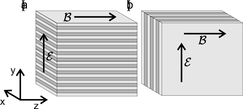
Figure 1: The orientations of the electric and magnetic field with respect to the superlattice structure. Configurations (a) and (b) are considered in sections III. and IV., respectively.

For Bloch oscillations, the very important issue is the intersubband tunneling of the Zener type. Lot of efforts were spent to clarify the condition under which Bloch oscillations could be observed and this problem is not yet definitely solved. ne ; so ; ya06 ; ya05 The same question needs to be addressed to the alternative magnetic-field-induced oscillations as we did not pay enough attention to this point in our previous publication. or

We will study the electrons in the presence of crossed magnetic and electric fields and subject to a unidirectional potential with the period determined by the lattice vector $\vec{a}$ oriented in the growth direction of the superlattice. The considered geometrical arrangements of the fields and the superlattice are shown in Fig. 1. The magnetic field acts in the direction $z$ with a constant intensity $\mathcal{B}$ and the electric field of a constant intensity $\mathcal{E}$ is parallel with the $y$ axis. Two directions of the lattice vector are considered with respect to the orientation of $\vec{\mathcal{E}}$: the parallel one, $\vec{a}\equiv(0,a,0)$, with the periodic potential potential $V(y)=V(y+a)$, and the perpendicular one, $\vec{a}\equiv(a,0,0)$, with the periodic potential $V(x)=V(x+a)$. The former configuration corresponds to the Bloch oscillations, the latter one to the alternative oscillations.

While the three-dimensional superlattices subject to in-plane electric and magnetic fields have been proposed as an alternative source of the terahertz oscillations, in our theoretical analysis the simpler two-dimensional model is employed. As the $z$-dependent part of the three-dimensional Hamiltonian, $p_{z}^{2}/2m$, does not play any role in the following theoretical consideration, we can omit it for simplicity without loss of generality.

II A free electron in crossed fields

We start with description of a free electron in crossed fields. davies In general, the two-dimensional Hamiltonian of an electron in the electromagnetic field reads

$$H=\frac{1}{2m}\left(\vec{p}-e\vec{A}\right)^{2}+e\,\phi,$$ (1)

where

$$\vec{\mathcal{E}}=-{\rm grad}\,\phi,\,\,\,\vec{\mathcal{B}}={\rm curl}\,\vec{A},$$ (2)

and $e=-|e|$. If we further assume $\phi=-\mathcal{E}\,y$ and employ the Landau gauge of the vector potential $\vec{A}=(-\mathcal{B}\,y,0,0)$, the Hamiltonian (1) reduces to

$$H_{0}=\frac{1}{2m}\left(p_{x}-|e|\mathcal{B}\,y\right)^{2}+\frac{p_{y}^{2}}{2m}+|e|\mathcal{E}\,y.$$ (3)

Since $H_{0}$ commutes with $p_{x}$, the separation of variables in the corresponding Schrödinger equation is possible.

The eigenvalues and eigenstates of $H_{0}$ are only slightly different from the more frequently described zero-electric-field case

$$\widetilde{H}_{0}=\frac{1}{2m}\left(p_{x}-|e|\mathcal{B}\,y\right)^{2}+\frac{p_{y}^{2}}{2m}.$$ (4)

The eigenfunctions of $\widetilde{H}_{0}$ can be written in the form

$$\psi_{0nk_{x}}(\vec{r})=\frac{1}{\sqrt{L_{x}}}{\mathrm{e}}^{ik_{x}x}\varphi_{0nk_{x}}(y),$$ (5)

where $k_{x}=j\,2\pi/L_{x},\,\,j=1,2,\cdots,N$ and the eigenenergies read

$$\widetilde{E}_{0n}(k_{x})=\hbar\omega\left(n+\frac{1}{2}\right),\,\,\ \omega=\frac{|e|\mathcal{B}}{m},\,\,n=0,1,\cdots.$$ (6)

$L_{x}$ and $L_{y}$ denote the sample dimensions.

The functions $\varphi_{0nk_{x}}(y)$ are the eigenfunctions of the harmonic oscillator,

$$\varphi_{0nk_{x}}(y)=\frac{1}{\sqrt{2^{n}n!\sqrt{\pi}\ell}}\,\exp{\left[-\frac{(y-y_{0})^{2}}{2\ell^{2}}\right]}H_{n}\left(\frac{y-y_{0}}{\ell}\right),$$ (7)

where $H_{n}$ are the Hermit polynomials and $\ell^{2}=\hbar/m\omega$. The coordinate $y_{0}=\ell^{2}k_{x}$ relates the center of the cyclotron orbit, given by $\langle\varphi_{0nk_{x}}|y|\varphi_{0nk_{x}}\rangle=y_{0}$, to the wave vector $k_{x}$, $y_{0}\in(0,L_{y})$. Since $k_{x}\in(0,L_{y}/\ell^{2})$ the number of states in a Landau level is given by $N=L_{x}L_{y}/2\pi\ell^{2}$ and the level degeneracy reads

$$\frac{N}{L_{x}L_{y}}=\frac{|e|\mathcal{B}}{h}.$$ (8)

Very similar form of the eigenstates of the full Hamiltonian $H_{0}$ is obtained if we sum in Eq. (3) the terms linear and quadratic in $y$. Then $H_{0}$ takes the form

$$H_{0}=\frac{1}{2m}\left(p_{x}-mv_{d}-|e|\mathcal{B}\,y\right)^{2}$$ (9)

$$\mbox{}+\frac{p_{y}^{2}}{2m}+v_{d}(p_{x}-mv_{d})+\frac{mv_{d}^{2}}{2},$$

in which the drift velocity $v_{d}=\mathcal{E}/\mathcal{B}$ of an electron in crossed fields is employed.

It follows from the similarity between expressions (4) and (9) that the eigenenergies of $H_{0}$ can be constructed from the zero-electric-field ones, $\widetilde{E}_{0n}(k_{x})$, given by Eq. (6). They can be expressed as

$$E_{0n}(\bar{k}_{x})=\widetilde{E}_{0n}(\bar{k}_{x})+\hbar\bar{k}_{x}v_{d}+\frac{mv_{d}^{2}}{2},$$ (10)

where $\bar{k}_{x}$ stands for $k_{x}-mv_{d}/\hbar$. The Landau levels become tilted and, therefore, their degeneracy in $k_{x}$ is lifted. The eigenfunctions $\varphi_{0n\bar{k}_{x}}(y)$ remain practically unchanged, only the wave vector $k_{x}$ was replaced by $\bar{k}_{x}$ in Eq. (7).

In comparison with the zero-electric-field case the diagonal matrix element of the velocity component is nonzero and given by

$$\langle\varphi_{0n\bar{k}_{x}}|v_{x}|\varphi_{0n\bar{k}_{x}}\rangle=\frac{1}{\hbar}\frac{\partial E_{n}(\bar{k}_{x})}{\partial\bar{k}_{x}}=v_{d},$$ (11)

and the center of mass of the cyclotron orbit reads $\langle\varphi_{0n\bar{k}_{x}}|y|\varphi_{0n\bar{k}_{x}}\rangle=\ell^{2}\bar{k}_{x}=y_{0}-v_{d}/\omega$.

This well known example demonstrates that the electric field does change the zero-electric-field electronic structure only in an unessential way. Both systems are described by almost equivalent Hamiltonians which differ only by the shift of the coordinate center and the changes of the constants. We will show in the following sections that it is valid also in the presence of the superlattice periodic potential.

III The electric field parallel with the lattice vector

In the zero-magnetic-field limit this geometrical arrangement would lead to the standard Bloch oscillations. In crossed electric and magnetic fields the Hamiltonian can be written as a sum of $H_{0}$, as given by Eq. (9), and of the periodic potential $V(y)$,

$$H=H_{0}+V(y).$$ (12)

The resulting Hamiltonian reads

$$H=\frac{1}{2m}\left(p_{x}-mv_{d}-|e|\mathcal{B}\,y\right)^{2}$$ (13)

$$\mbox{}+\frac{p_{y}^{2}}{2m}+V(y)+v_{d}(p_{x}-mv_{d})+\frac{mv_{d}^{2}}{2}.$$

Similarly as in the case of a free electron described above, it is obvious that the eigenstates of $H$ are closely related to the eigenstates of the zero-electric-field Hamiltonian

$$\widetilde{H}=\frac{1}{2m}\left(p_{x}-|e|\mathcal{B}\,y\right)^{2}+\frac{p_{y}^{2}}{2m}+V(y).$$ (14)

For a given $k_{x}$ both Hamiltonians reduce to one-dimensional ones, which differ only by a constant $v_{d}\bar{k}_{x}+{mv_{d}^{2}}/{2}$ and a shift $mv_{d}/\hbar$ in the wave vector $k_{x}$. Therefore both Hamiltonians yield essentially the same spectrum of eigenvalues.

The eigenenergies of the Hamiltonian (13) can be written, in analogy with Eq. (10), as

$$E_{s}(\bar{k}_{x})=\widetilde{E}_{s}(\bar{k}_{x})+\hbar\bar{k}_{x}v_{d}+\frac{mv_{d}^{2}}{2}.$$ (15)

Note that for the zero-electric-field case the periodic potential $V(y)$ removes the degeneracy of Landau levels. The eigenenergies of the Hamiltonian (14) become the Landau subbands $\widetilde{E}_{s}(k_{x})$, $s=0,1,2,\cdots$, periodic in $k_{x}$ with the period

$$K=\frac{a}{\ell^{2}}=\frac{a|e|\mathcal{B}}{\hbar}.$$ (16)

We replace $n$ by the integer $s$ to distinguish between a subband and a level. The corresponding eigenfuctions $\widetilde{\varphi}_{s}(k_{x})$ are, similarly as $\varphi_{0nk_{x}}$, bounded in $y$ direction for any $k_{x}$ due to the confinement by the parabolic potential generated by $\mathcal{B}$.

The diagonal matrix elements of the velocity component $v_{x}$ in crossed fields are now given by

$$\langle\widetilde{\varphi}_{s\bar{k}_{x}}|v_{x}|\widetilde{\varphi}_{s\bar{k}_{x}}\rangle=\frac{1}{\hbar}\frac{\partial E_{s}(\bar{k}_{x})}{\partial\bar{k}_{x}}=\frac{1}{\hbar}\frac{\partial\widetilde{E}_{s}(\bar{k}_{x})}{\partial\bar{k}_{x}}+v_{d},$$ (17)

and the center of mass of the cyclotron orbit reads

$$\langle\widetilde{\varphi}_{s\bar{k}_{x}}|y|\widetilde{\varphi}_{s\bar{k}_{x}}\rangle=y_{0}-v_{d}/\omega-\frac{1}{\hbar\omega}\frac{\partial\widetilde{E}_{s}(\bar{k}_{x})}{\partial\bar{k}_{x}}.$$ (18)

It follows from Eq. (15) that $E_{s}(\bar{k}_{x})$ is a step-like function with the step length $K$ and the step height $|e|\mathcal{E}a$, i.e. we can write

$$E_{s}(\bar{k}_{x}+K)=E_{s}(\bar{k}_{x})+\hbar\omega_{BO},\,\,\,\,\,\omega_{BO}=\frac{|e|\mathcal{E}a}{\hbar},$$ (19)

where $\omega_{BO}$ denotes the frequency of Bloch oscillations.

This step function replaces the standard Wannier-Stark ladder obtained in the zero-magnetic-field case. Note that $E_{s}(\bar{k}_{x})$ are the true eigenenergies and not the resonances as the Wannier-Stark states, i.e. the magnetic field completely suppresses the Zener tunneling.

The energy spectra of the above Hamiltonians can be found either by the direct numerical solution of the corresponding one-dimensional Schrödinger equations, or we can look for the eigenfunctions in the form of the linear combination of the free electron functions (7). As the resulting eigenenergies are the functions of $k_{x}$, we can evaluate the matrix elements for a given $k_{x}$ and diagonalize the resulting matrix.

The matrix elements of the Hamiltonian $\widetilde{H}$, Eq. (14), are diagonal in $k_{x}$. The periodic potential $V(y)$ can be expanded into the Fourier series,

$$V(y)=\sum_{j}V_{j}\cos(G_{j}y),$$ (20)

with $G_{j}=jG$, $G=2\pi/a$ being the reciprocal lattice vector. Therefore, we can look for the eigenfunctions $\widetilde{\varphi}_{sk_{x}}(y)$ in the form

$$\widetilde{\varphi}_{sk_{x}}=\sum_{n^{\prime}}c_{n^{\prime}}\psi_{0n^{\prime}k_{x}},$$ (21)

and the matrix elements of $\widetilde{H}$ can be written as

$$\widetilde{H}_{k_{x},n,n^{\prime}}=\hbar\omega\left(n+\frac{1}{2}\right)\delta_{n,n^{\prime}}+T_{k_{x},n,n^{\prime}},$$ (22)

where $T_{k_{x},n,n^{\prime}}$ is the matrix element of a component of the periodic potential

$$T_{k_{x},n,n^{\prime}}=$$ (23)

$$\sum_{j}V_{j}\frac{1}{\sqrt{2^{n}2^{n^{\prime}}n!n^{\prime}!\pi\ell^{2}}}\int_{-\infty}^{+\infty}\exp\left[{-\frac{(y-y_{0})^{2}}{\ell^{2}}}\right]$$

$$\times H_{n}\left(\frac{y-y_{0}}{\ell}\right)H_{n^{\prime}}\left(\frac{y-y_{0}}{\ell}\right)\cos\left(G_{j}y\right){\mathrm{d}}y.$$

Introducing the dimensionless variable $\eta=(y-y_{0})/\ell$, we obtain

$$T_{k_{x},n,n^{\prime}}=$$ (24)

$$\sum_{j}V_{j}\frac{1}{\sqrt{2^{n}2^{n^{\prime}}n!n^{\prime}!\pi}}\int_{-\infty}^{+\infty}\exp{\left(-\eta^{2}\right)}$$

$$\times H_{n}(\eta)H_{n^{\prime}}(\eta)\cos(G_{j}\ell\eta+G_{j}y_{0}){\mathrm{d}}\eta.$$

To reduce this expression to a pair of standard tabular integrals we can employ the simple trigonometric relation

$$cos(G_{j}\ell\eta+G_{j}y_{0})=$$ (25)

$$\cos(G_{j}\ell\eta)\cos(G_{j}y_{0})-\sin(G_{j}\ell\eta)\sin(G_{j}y_{0}).$$

After substitution, the examined $T_{k_{x},n,n^{\prime}}$ is divided into two parts $I_{1,n,n^{\prime}}$ and $I_{2,n,n^{\prime}}$. The first part, which includes the cosine in the integrand, is equal to zero if the integrand is the odd function. For the even integrand it reads

$$I_{1,n,n^{\prime}}=$$ (26)

$$\sum_{j}V_{j}\frac{2\cos(G_{j}y_{0})}{\sqrt{2^{n}2^{n^{\prime}}n!n^{\prime}!\pi}}\int_{0}^{+\infty}\exp{\left(-\eta^{2}\right)}$$

$$\times H_{n}(\eta)H_{n^{\prime}}(\eta)\cos(G_{j}\ell\eta){\mathrm{d}}\eta.$$

The explicit analytic form of $I_{1,n,n^{\prime}}$ (see,e.g., Gradshtejn ) is given by

$$I_{1,n,n^{\prime}}=$$ (27)

$$\sum_{j}V_{j}\,\sqrt{\frac{2^{n}n!}{2^{n^{\prime}}n^{\prime}!}}(-1)^{\frac{n^{\prime}-n}{2}}(G_{j}\ell)^{n^{\prime}-n}\exp\left(-\frac{G^{2}_{j}\ell^{2}}{4}\right)$$

$$\times L_{n}^{n^{\prime}-n}\left(\frac{G^{2}_{j}\ell^{2}}{2}\right)\cos(G_{j}y_{0}),$$

for $n^{\prime}-n=2p$. Here $L_{n}^{n^{\prime}-n}$ are the Laguerre polynomials, and $p$ is an integer number. The second part $I_{2,n,n^{\prime}}$ differs from the first one only by the sine written instead of the cosine

$$I_{2,n,n^{\prime}}=$$ (28)

$$-\sum_{j}V_{j}\frac{2\sin(G_{j}y_{0})}{\sqrt{2^{n}2^{n^{\prime}}n!n^{\prime}!\pi}}\int_{0}^{+\infty}\exp{\left(-\eta^{2}\right)}$$

$$\times H_{n}(\eta)H_{n^{\prime}}(\eta)\sin(G_{j}\ell\eta){\mathrm{d}}\eta.$$

The part $I_{2,n,n^{\prime}}$ is also given by the tabular integrals which are nonzero for the odd integrands

$$I_{2,n,n^{\prime}}=$$ (29)

$$-\sum_{j}V_{j}\sqrt{\frac{2^{n}n!}{2^{n^{\prime}}n^{\prime}!}}(-1)^{\frac{n^{\prime}-n-1}{2}}(G_{j}\ell)^{n^{\prime}-n-1}\exp\left(-\frac{G^{2}_{j}\ell^{2}}{4}\right)$$

$$\times L_{n}^{n^{\prime}-n}\left(\frac{G^{2}_{j}\ell^{2}}{2}\right)\sin(G_{j}y_{0}),$$

for $n^{\prime}-n=2p+1$. Note that $k_{x}$ enters the matrix elements $T_{k_{x},n,n^{\prime}}$ through the identity $G_{j}y_{0}=j2\pi k_{x}/K$. Only the minor changes are introduced by applying the electric field. The matrix elements of the Hamiltonian (13) read

$$H_{\bar{k}_{x},n,n^{\prime}}=\left[\hbar\omega\left(n+\frac{1}{2}\right)+\hbar\bar{k}_{xj}v_{d}+\frac{mv_{d}^{2}}{2}\right]\delta_{n,n^{\prime}}+T_{\bar{k}_{x},n,n^{\prime}}$$ (30)

The similarity between Hamiltonians (22) and (30) confirms the validity of the expression (15).

As a simple example Labbe we present the case of a weak perturbation $V(y)=V\cos(Gy)$ which does not mix the Landau levels with different $n$. Then, replacing $n$ by $s$ to stress the difference between the level and the subband, the eigenenergies for the zero-electric-field Hamiltonian become

$$\widetilde{E}_{s}(k_{x})=\hbar\omega\left(s+\frac{1}{2}\right)$$ (31)

$$+V\exp\left(-\frac{G^{2}\ell^{2}}{4}\right)L_{s}\left(\frac{G^{2}\ell^{2}}{2}\right)\cos\left(\frac{2\pi k_{x}}{K}\right),$$

and, finally, we get in accord with Eq. (15),

$${E}_{s}(\bar{k}_{x})=\hbar\omega\left(s+\frac{1}{2}\right)+\hbar\bar{k}_{x}v_{d}+\frac{mv_{d}^{2}}{2}$$ (32)

$$+V\exp\left(-\frac{G^{2}\ell^{2}}{4}\right)L_{s}\left(\frac{G^{2}\ell^{2}}{2}\right)\cos\left(\frac{2\pi\bar{k}_{x}}{K}\right),$$

for the eigenvalues in the electric field.

IV The electric field perpendicular to the lattice vector

This arrangement corresponds to the alternative oscillations. The Hamiltonian of an electron in crossed electric and magnetic fields with the periodic modulation in the $x$ direction can be written as a sum of the Hamiltonian $H_{0}$, as given by Eq. (9), and of the potential $V(x)$,

$$H=H_{0}+V(x),$$ (33)

or, explicitly,

$$H=\frac{1}{2m}\left(p_{x}-mv_{d}-|e|\mathcal{B}\,y\right)^{2}$$ (34)

$$\mbox{}+\frac{p_{y}^{2}}{2m}+V(x)+v_{d}(p_{x}-mv_{d})+\frac{mv_{d}^{2}}{2}.$$

We expect that due to the strong confinement by the magnetic field the eigenfunctions will be localized in $y$ direction. For $\mathcal{E}\rightarrow 0$, the eigenenergies should reduce to $\widetilde{E}_{s}(k_{y})$, periodic in $k_{y}$ with the period $K$. This function must be equivalent to $\widetilde{E}_{s}(k_{x})$ found in the previous section, as the result should not depend on the choice of calibration of the vector potential.

Since the Hamiltonian (34) cannot be simply reduced to the one-dimensional one, we will look for the eigensolutions starting from the linear combination of eigenfunctions of $H_{0}$. The potential $V(x)$ will be, similarly as in Sec. III, considered in the form of the Fourier series

$$V(x)=\sum_{j}V_{j}\cos(G_{j}x).$$ (35)

The functions $\psi_{s\bar{k}_{x}}(\vec{r})$, we are looking for, can be written as a Bloch sum,

$$\psi_{s\bar{k}_{x}}(\vec{r})=\sum_{n^{\prime}j^{\prime}}c_{n^{\prime}j^{\prime}}{\mathrm{e}}^{i\bar{k}_{xj^{\prime}}x}\varphi_{0n^{\prime}\bar{k}_{xj^{\prime}}}(y),$$ (36)

where $\bar{k}_{xj}=\bar{k}_{x}+G_{j}$, i.e. as the linear combination of functions the centers of which, $\ell^{2}\bar{k}_{xj}$, are arranged periodically along the $y$ axis with the distance $\ell^{2}G$.

For a given $\bar{k}_{x}$, the matrix elements of the Hamiltonian (34) can be written as

$$H_{\bar{k}_{x},nj,n^{\prime}j^{\prime}}=$$

$$\left[\hbar\omega\left(n+\frac{1}{2}\right)+\hbar\bar{k}_{xj^{\prime}}v_{d}+\frac{mv_{d}^{2}}{2}\right]\delta_{nj,n^{\prime}j^{\prime}}+T_{nj,n^{\prime}j^{\prime}}.$$

Here $T_{nj,n^{\prime}j^{\prime}}$ denotes the matrix elements of the potential $V(x)$. They are products of the matrix elements of $V_{j}\cos(G_{j}x)$, calculated between the plane-wave parts of the wave functions, and of the overlap integrals of localized functions $\varphi_{0n^{\prime}\bar{k}_{xj^{\prime}}}(y)$. Only the matrix elements $V_{j-j^{\prime}}$ are nonzero. The centers of overlapping functions are $\ell^{2}\bar{k}_{xj}$ and $\ell^{2}\bar{k}_{xj^{\prime}}$, respectively, and their distance is $\ell^{2}G_{j-j^{\prime}}$. Then $T_{nj,n^{\prime}j^{\prime}}$ are equal to

$$T_{nj,n^{\prime}j^{\prime}}=V_{j-j^{\prime}}\sqrt{\frac{2^{n^{\prime}}n!}{2^{n}n^{\prime}!}}\exp\left(-\frac{G^{2}_{j-j^{\prime}}\ell^{2}}{4}\right)$$ (38)

$$\times\left(\frac{G_{j-j^{\prime}}\ell}{2}\right)^{n^{\prime}-n}L_{n}^{n^{\prime}-n}\left(\frac{G^{2}_{j-j^{\prime}}\ell^{2}}{2}\right)$$

for $n^{\prime}\geq n$ and

$$T_{nj,n^{\prime}j^{\prime}}=V_{j-j^{\prime}}\sqrt{\frac{2^{n}n^{\prime}!}{2^{n^{\prime}}n!}}\exp\left(-\frac{G^{2}_{j-j^{\prime}}\ell^{2}}{4}\right)$$ (39)

$$\times\left(-\frac{G_{j-j^{\prime}}\ell}{2}\right)^{n-n^{\prime}}L_{n^{\prime}}^{n-n^{\prime}}\left(\frac{G^{2}_{j-j^{\prime}}\ell^{2}}{2}\right)$$

for $n^{\prime}\leq n$. They decrease exponentially with the distance between the centers of functions $\varphi_{0n\bar{k}_{xj}}(y)$ and $\varphi_{0n^{\prime}\bar{k}_{xj^{\prime}}}(y)$.

Note that the electric field $\mathcal{E}$ (the drift velocity $v_{d}$) and the wave vector $\bar{k}_{x}$ enter only the diagonal part of the Hamiltonian, and, therefore, only the diagonal elements of the corresponding matrix equation which reads

$$\sum_{n^{\prime}j^{\prime}}\left(H_{\bar{k}_{x},nj,n^{\prime}j^{\prime}}-E\right)c_{n^{\prime}j^{\prime}}=0.$$ (40)

This allows us to predict an interesting $\bar{k}_{x}$ dependence of the eigenstates of the above equation.

First, it follows from the form of the matrix elements of the Hamiltonian (IV) that the eigenenergies depend linearly on $\bar{k}_{x}$, and that the electrons move, in spite of the presence of the superlattice potential, with the same drift velocity $v_{d}$ as free electrons in crossed fields. Moreover, if we replace $\bar{k}_{x}$ by $\bar{k}_{x}+G$, we can rewrite the Hamiltonian matrix elements (IV) to the form

$$H_{\bar{k}_{x}+G,nj,nj}=H_{\bar{k}_{x},nj,nj}+\hbar Gv_{d}.$$ (41)

Then equation

$$\sum_{n^{\prime}j^{\prime}}\left(H_{\bar{k}_{x}+G,nj,n^{\prime}j^{\prime}}-E\right)c_{n^{\prime}j^{\prime}}=0$$ (42)

can be replaced by

$$\sum_{n^{\prime}j^{\prime}}\left(H_{\bar{k}_{x},nj,n^{\prime}j^{\prime}}-E^{\prime}\right)c_{n^{\prime}j^{\prime}}=0$$ (43)

where $E^{\prime}$ stands for $E-\hbar Gv_{d}$. Therefore we can conclude for the corresponding eigenvalues that

$$E_{s}(k_{x}+G)=E_{s}(k_{x})+\hbar\omega_{\mathcal{B_{\parallel}}},\,\,\omega_{\mathcal{B_{\parallel}}}=\frac{2\pi v_{d}}{a}.$$ (44)

The eigenvalues of Eq. (40) should reduce for $\mathcal{E}\rightarrow 0$ to the zero-field eigenvalues $\widetilde{E}_{s}$ periodic in $k_{y}$.

We will again illustrate the above consideration on the simple case of a weak perturbation $V\cos(Gx)$.

We start with the case of the zero electric field Labbe to show how the $k_{y}$ dependence of $\widetilde{E}_{s}$ is introduced.

The function

$$\widetilde{\psi}_{sk_{x}}(\vec{r})=\sum_{j^{\prime}}c_{j^{\prime}}{\mathrm{e}}^{ik_{xj^{\prime}}x}\varphi_{0nk_{xj^{\prime}}}(y)=\sum_{j^{\prime}}c_{j^{\prime}}|nj^{\prime}\rangle$$ (45)

is assumed not to mix the Landau levels. Note that $k_{x}\in(-\pi/a,\pi/a)$ and $j^{\prime}=1,2,\cdots,j_{M}$ where $j_{M}=L_{y}a/2\pi\ell^{2}$. The equation

$$\langle nj|H-E|\widetilde{\psi}_{sk_{x}}\rangle=0$$ (46)

implies

$$c_{j}\left[\hbar\omega\left(n+\frac{1}{2}\right)-E\right]$$

$$+\frac{V}{2}\exp\left(-\frac{G^{2}\ell^{2}}{4}\right)L_{n}\left(\frac{G^{2}\ell^{2}}{2}\right)\left(c_{j-1}+c_{j+1}\right)=0.$$

We write $c_{j}$ in the form $c_{j}=c_{0}\exp(iqj)$ and look for $c_{0}$ and $q$ instead of $c_{j}$. The first consequence is that the solution of Eq. (46) can be written in the form

$$\widetilde{E}_{s}=\hbar\omega\left(n+\frac{1}{2}\right)+V\exp\left(-\frac{G^{2}\ell^{2}}{4}\right)L_{n}\left(\frac{G^{2}\ell^{2}}{2}\right)\cos q.$$ (48)

It follows from $\langle\widetilde{\psi}_{sk_{x}}|\widetilde{\psi}_{sk_{x}}\rangle=1$ that $j_{M}c_{0}^{2}=1$ and $c_{0}^{2}=\ell^{2}G/L_{y}$.

If we write $\widetilde{\psi}_{sk_{x},q}$ as

$$\widetilde{\psi}_{sk_{x},q}=c_{0}\sum_{j^{\prime}}{\mathrm{e}}^{iqj^{\prime}}|nj^{\prime}\rangle$$ (49)

we get from

$$\langle\widetilde{\psi}_{sk_{x},q}|\widetilde{\psi}_{sk_{x},q^{\prime}}\rangle=0$$ (50)

the expression $q=(2\pi\nu/L_{y})\ell^{2}G,\nu=1,2,\cdots$. Taking into account that $2\pi\nu/L_{y}=k_{y}$ and $x_{0}=\ell^{2}k_{y}$, we arrive at $q=x_{0}G=2\pi k_{y}/K$ and finally

$$\widetilde{E}_{s}(k_{y})=\hbar\omega\left(s+\frac{1}{2}\right)$$ (51)

$$+V\exp\left(-\frac{G^{2}\ell^{2}}{4}\right)L_{s}\left(\frac{G^{2}\ell^{2}}{2}\right)\cos\left(\frac{2\pi k_{y}}{K}\right).$$

As expected, the change of the direction of the lattice vector has no influence and the only difference in comparison with the $V(y)$ case, see Eq. (31), is replacement of $k_{x}$ by $k_{y}$.

It is not too difficult to introduce the electric field into this simple model. First, the $k_{x}$ must be replaced by $\bar{k}_{x}$ and $q$ by $k_{y}=Kq/2\pi$ in $\widetilde{\psi}_{s{k}_{x},q}$. Then we can calculate the matrix elements of the Hamiltonian (IV), which include the $\bar{k}_{x}$ and $v_{d}$ dependent parts. We get

$$\langle\widetilde{\psi}_{s\bar{k}_{x},q}|H|\widetilde{\psi}_{s\bar{k}_{x},q^{\prime}}\rangle=$$ (52)

$$\delta_{k_{y},k^{\prime}_{y}}\left[\widetilde{E}_{s}(k_{y})+\hbar\bar{k}_{x}v_{d}+\frac{mv_{d}^{2}}{2}-i|e|\mathcal{E}\frac{d}{dk_{y}}\right],$$

and thus, taking into account the periodicity in $k_{y}$, the eigenenergies of the corresponding equation can be easily calculated:

$$E_{r,s,\bar{k}_{x}}=\frac{1}{K}\int_{0}^{K}\widetilde{E}_{s}(k_{y})dk_{y}$$ (53)

$$+\hbar\bar{k}_{x}v_{d}+\frac{mv_{d}^{2}}{2}+r\hbar\omega_{\mathcal{B_{\parallel}}},\,\,\,r=0,\pm 1,\cdots.$$

In this example we limited our consideration to one subband $\widetilde{E}_{s}(k_{y})$. Note that for more subbands the electric field cannot cause the intersubband transition, as we use the electric-field-dependent basis of functions ${\mathrm{e}}^{i\bar{k}_{xj^{\prime}}x}\varphi_{0n^{\prime}\bar{k}_{xj^{\prime}}}(y)$. Therefore, the solutions of Eq. (40) are the eigenstates and not the resonances.

V Conclusions

The presented theoretical analysis has implicitly assumed a single electron model for a Bloch electron in crossed electric and magnetic fields, $\vec{\mathcal{E}}\perp\vec{\mathcal{B}}$, moving in a perfect superlattice crystal with the lattice vector $\vec{a}$. Two geometrical arrangements were considered.

In the case $\vec{a}\parallel\vec{\mathcal{E}}$, which would correspond to the Bloch oscillations for $\mathcal{B}=0$, the magnetic field converts the standard Wannier-Stark ladder of resonances to the step-like eigenenergies, which are functions of the wave vector $\vec{k}_{\perp}$, perpendicular to both $\vec{\mathcal{E}}$ and $\vec{\mathcal{B}}$. The step length is $a|e|\mathcal{B}/\hbar$. The step height $\hbar\omega_{BO}$ corresponds to the frequency of the Bloch oscillations $\omega_{BO}=|e|\mathcal{E}a/\hbar$.

The alternative magnetic-field-induced oscillations were suggested as a possible source of terahertz radiation or for the case $\vec{a}\perp\vec{\mathcal{E}}$. The electron motion is composed from oscillations along $\vec{a}$ and the drift due to the Lorentz force with the velocity $v_{d}=\mathcal{E}/\mathcal{B}$ in the direction of $\vec{k}_{\perp}$. The resulting eigenstates resemble those of a free electron in crossed fields. The eigenenergies $E_{M}$ depends linearly on the $k_{\perp}$, $E_{M}\propto\hbar v_{d}k_{\perp}$, their separation on the energy scale is $\hbar\omega_{\mathcal{B_{\parallel}}}$.

The above conclusions are valid for the optimal conditions for coherent Bloch and alternative oscillations, neglecting the importance of additional scattering which can lead to damping of oscillations.

VI Acknowledgements

This work has been supported by the Ministry of Education of the Czech Republic Center for Fundamental Research LC510, the Ministry of Education of the Czech Republic research plan MSM 0021620834, and Academy of Sciences of the Czech Republic project KAN400100652.

References

• (1) J.  Faist, F. Capasso, D. L. Sivco, C. Sirtori, A. L. Hutchinson and A. Y. Cho, Science 264, 553 (1994).
• (2) J. Feldmann, K. Leo, J. Shah, D. A. B. Miller, J. E. Cunningham, T. Meier, G. von Plessen, A. Schulze, P. Thomas, and S. Schmitt-Rink, Phys. Rev. B 46, 7252 (1992).
• (3) C. Waschke, H. G. Roskos, R. Schwedler, K. Leo, H. Kurz, and K. Köhler, Phys. Rev. Lett. 70, 3319 (1993).
• (4) T. Dekorsy, P. Leisching, K. Köhler, and H. Kurz, Phys. Rev. B 50, 8106 (1994).
• (5) G. C. Cho, T. Dekorsy, H. J. Bakker, H. Kurz, A. Kohl, and B. Opitz, Phys. Rev. B 54 4420 (1996).
• (6) V. G. Lyssenko, G. Valusis, F. Löser, T. Hasche, K. Leo, M. M. Dignam, and K. Köhler, Phys. Rev. Lett. 79, 301 (1997).
• (7) T. Hartmann, F. Keck, H. J. Korsch, and S. Mossmann, New J. Phys. 6, 2 (2004).
• (8) K. Leo, Semicond. Sci. Technol. 13 249 (1998).
• (9) A. Patanè, N. Mori, D. Fowler, L. Eaves, M. Henini, D. K. Maude, C. Hamaguchi, and R. Airey, Phys. Rev. Lett. 93, 146801 (2004).
• (10) G. Scalari, S. Blaser,J. Faist, H. Beere, E. Linfield, D. Ritchie, and G. Davies, Phys. Rev. Lett. 93, 237403 (2004).
• (11) M. Orlita, R. Grill, L. Smrčka, and M. Zvára, Phys. Rev. B 74, 125312 (2006).
• (12) N. Qureshi, “Terahertz Dynamics of a Superlattice in Crossed Electric and Magnetic Fields” Ph.D. thesis, University of California, Santa Barbara, 2002.
• (13) C. Wang and J. C. Cao, Phys. Rev. B 72, 045339 (2005).
• (14) T. M. Fromhold, A. A. Krokhin, C. R. Tench, S. Bujkiewicz, P. B. Wilkinson, F. W. Sheard, and L. Eaves, Phys. Rev. Lett. 87, 046803 (2001).
• (15) T. M. Fromhold, A. Patanè, S. Bujkewicz, P. B. Wilkinson, D. Fowler, D. Sherwood, S. P. Stapleton, A. A. Krokhin, L. Eaves, M. Henini, N. S. Sankeshwar, and F. W. Sheard, Nature (London) 428, 726 (2004).
• (16) G. Nenciu, Rev. Mod. Phys. 63, 91 (1991).
• (17) V. N. Sokolov, L. Zhou, G. J. Iafrate, and J. B. Krieger, Phys. Rev. B 73, 205304 (2006).
• (18) Lijun Yang and Marc M. Dignam, Phys. Rev. B 73, 075319 (2006).
• (19) Lijun Yang, Ben Rosam, K. Leo, and Marc M. Dignam, Phys. Rev. B 72, 115313 (2005).
• (20) J. H. Davies, The Physics of Low-Dimensional Semiconductors: An Introduction (Cambridge University Press, Cambridge 1997), p. 229.
• (21) I. S. Gradshteyn, I. M. Ryzhik, Tables of integrals, sums, series, and products (Moscow, 1963), p. 852-855.
• (22) J. Labbé, Phys. Rev. B 35, 1373 (1987).