Isoperimetric inequalities for eigenvalues of triangles

Abstract.

Lower bounds estimates are proved for the first eigenvalue for the Dirichlet Laplacian on arbitrary triangles using various symmetrization techniques. These results can viewed as a generalization of Pólya’s isoperimetric bounds. It is also shown that amongst triangles, the equilateral triangle minimizes the spectral gap and (under additional assumption) the ratio of the first two eigenvalues. This last result resembles the Payne-Pólya-Weinberger conjecture proved by Ashbaugh and Benguria.

1. Introduction

The purpose of this paper is to prove new isoperimetric–type bounds for the eigenvalues of the Dirichlet Laplacian on arbitrary triangles. Given a domain $D$ we will use “eigenvalue of the domain $D$” to refer to an eigenvalue of the Dirichlet Laplacian on the domain $D$. The eigenvalues for a domain form a nondecreasing sequence $\{\lambda_{i},j\geq 1\}$ with $\lambda_{1}<\lambda_{2}$. Throughout the paper we use $A$ for the area of a domain, $L$ for its perimeter, $R$ for its inradius (the supremum of the radii of disks contained in the domain) and $d$ for its diameter.

The problem of finding good bounds for eigenvalues of various domains has been of interest for many years. See for example [PS, Du, AB, Pr] for general bounds, [S2, AF] for result about polygons, and [F, F2, S] for bounds for triangles. Comprehensive overview of this subject along with methods used to tackle it can be found in the book [H]. The results contained in [F2] are especially interesting, since they are of different nature than our bounds and it should be possible to combine methods from this paper with our approach to get even better bounds.

In [PS]*Section 7.4, Pólya and Szegö conjectured that with fixed area, amongst all polygons with $n$ sides the regular one minimizes the first eigenvalue (they also conjectured that the inner radius and the transfinite diameter are also minimized, but these has been proved). The conjecture remains open except for the following cases:

(1.1) $$\lambda_{1}A|_{Triangle}\geq\lambda_{1}A|_{Equilateral},$$

(1.2) $$\lambda_{1}A|_{Quadrilateral}\geq\lambda_{1}A|_{Square},$$

(1.3) $$\lambda_{1}A\geq\lambda_{1}A|_{Ball}.$$

The notation $|_{set}$ is used to indicate the set for the quantity to the left of it. In the last bound (called the Faber-Krahn inequality) no set is specified since the bound is true for an arbitrary domain. The proofs of these results along with the conjecture for polygons can be found in [H]. Note that the ball in the last bound can be viewed as a limiting case of a regular polygon with an infinite number of sides.

There are also upper bounds where in this case the ball is the extremal.

(1.4) $$\lambda_{1}R^{2}\leq\lambda_{1}R^{2}|_{Ball},$$

(1.5) $${\lambda_{2}\over\lambda_{1}}\leq\left.{\lambda_{2}\over\lambda_{1}}\right|_{Ball},$$

(1.6) $$(\lambda_{2}-\lambda_{1})R^{2}\leq(\lambda_{2}-\lambda_{1})R^{2}|_{Ball}.$$

The first inequality follows trivially from the domain monotonicity. The second and the third are known as the Payne-Pólya-Weinberger conjecture proved by Ashbaugh and Benguria [AB]. Note that there is no scaling factor (area or inradius) in the second bound. The difference of the eigenvalues in the last bound is called the spectral gap and it is important in the study of dynamical systems. It can be regarded as a measure of the speed of convergence to equilibrium. For more on this, see [bame] and [smits].

We can see that a ball gives both upper and lower bounds for general domains. We want to show that an equilateral triangle has exactly the same properties among triangles. We already have the lower bound (1.1) as an analog of (1.3). It is proved in [S] that

(1.7) $$\lambda_{1}R^{2}|_{Triangle}\leq\lambda_{1}R^{2}|_{Equilateral}.$$

This is the parallel of the bound (1.4). The first result of this paper is the following

Theorem 1.1.

For arbitrary triangle

(1.8) $$(\lambda_{2}-\lambda_{1})R^{2}|_{Triangle}\leq(\lambda_{2}-\lambda_{1})R^{2}|_{Equilateral}.$$

If a triangle is acute we also have

(1.9) $$\left.{\lambda_{2}\over\lambda_{1}}\right|_{Triangle}\leq\left.{\lambda_{2}\over\lambda_{1}}\right|_{Equilateral}.$$

The additional assumption in the second part of the theorem is due to the method used to prove the result. We believe this result should hold for all triangles. The proof of the theorem relies on a variational formula for eigenvalues, as well as some very cumbersome computations.

In view of these results, we venture to propose the following generalization of Pólya’s conjecture about polygons

Conjecture 1.2.

Let $P(n)$ denote a polygon with $n$ sides and $R(n)$ a regular polygon with $n$ sides. Then

(1.10) $$\lambda_{1}A|_{P(n)}\geq\lambda_{1}A|_{R(n)},$$

(1.11) $$\lambda_{1}R^{2}|_{P(n)}\leq\lambda_{1}R^{2}|_{R(n)},$$

(1.12) $$(\lambda_{2}-\lambda_{1})R^{2}|_{P(n)}\leq(\lambda_{2}-\lambda_{1})R^{2}|_{R(n)},$$

(1.13) $$\left.{\lambda_{2}\over\lambda_{1}}\right|_{P(n)}\leq\left.{\lambda_{2}\over\lambda_{1}}\right|_{R(n)}.$$

It is easy to check that this conjecture is true for rectangles and that for quadrilaterals (1.10) is the same as (1.2). Our results along with (1.1) and (1.7) prove this conjecture for triangles, except for obtuse triangles in the last bound. All other cases remain open. It is worth noting that a slightly weaker version of (1.11) is a part of [S2]*Theorem 2. The only difference is that the scaling factor $R$ is missing and the regular polygon has outer radius $1$ instead of inradius $1$. As we have been recently informed by the author of [S2], the proof of this theorem should work if we replace outer radius $1$ with inradius $1$. This would prove inequality (1.11).

The second goal of this paper is to establish sharper lower bounds for the first eigenvalues of arbitrary triangles. In addition to (1.1) we have

(1.14) $$\lambda_{1}\geq\frac{\pi^{2}}{4}\left(R^{-2}+d^{-2}\right),$$

(1.15) $$\lambda_{1}\geq\pi^{2}\left(\frac{4}{d^{2}}+\frac{d^{2}}{4A^{2}}\right).$$

The first bound is due to Protter [Pr] and the second result was proved recently by Freitas [F]. Each of these bounds is the better than the other bounds for certain triangles, but not as good for some others.

We obtained new lower bounds for triangles which are better than (1.14) and (1.15) whenever these are better than (1.1).

Theorem 1.3.

For an arbitrary triangle with area $A$, diameter $d$ and shortest altitude $h$,

(1.16) $$\lambda_{1}|_{Triangle}\geq\pi^{2}\left(\frac{4}{d^{2}+h^{2}}+\frac{d^{2}+h^{2}}{4A^{2}}\right).$$

We also obtained a sharp bound based on circular sectors.

Theorem 1.4.

Let $\gamma$ be the smallest angle of a triangle. Denote by $I(A,\gamma)$ an isosceles triangle with same area $A$ and the vertex angle $\gamma$, and $S(A,\gamma)$ a circular sector with area $A$ and angle $\gamma$. Then

(1.17) $$\lambda_{1}|_{Triangle}\geq\lambda_{1}|_{I(A,\gamma)}\geq\lambda_{1}|_{S(A,\gamma)}.$$

The function

(1.18) $$f(\gamma)=\lambda_{1}|_{I(A,\gamma)}$$

is decreasing for $\gamma\in(0,\pi/3)$ and increasing for $\gamma\in(\pi/3,\pi)$.

This last result can be viewed as a generalization of the Pólya’s isoperimetric bound (1.1). If we fix $A$ and the smallest angle, then the isosceles triangle minimizes the first eigenvalue. Then, due to the monotonicity property, we also get an alternative prove of (1.1). The bounds involving circular sectors can be used to get good lower bounds for the eigenvalues since the eigenvalues of sectors are given explicitly in terms of the zeros of the Bessel function.

From now on $I(A,\gamma)$ will always denote an isosceles triangle with area $A$ and angle $\gamma$ between its sides of equal length. This angle will be called the vertex angle. The side opposite to that angle will be called the base and the other two the arms.

The methods used to prove (1.15) and (1.14) are not based on any kind of symmetrization argument. In contrast, the proofs of our lower bounds rely on certain symmetrization techniques similar to those used in the proof of Pólya’s isoperimetric inequality. In this sense, our results can be viewed as generalized isoperimetric bounds. Using the same techniques we also give an alternative proof of Freitas’s bound (1.15). This shows that symmetrization is the best way for obtaining lower bounds for the eigenvalues, at least for triangles. The bound is determined by the shape of the symmetrized domains. That is, the equilateral triangle in (1.1), the rectangles in Theorem 1.3 and (1.15), or the circular sector in Theorem 1.4.

The rest of the paper is organized as follows. In Section 2 we compare the new lower bounds with the known results. Section 3 contains the definitions and basic explanations of various forms of symmetrization techniques which are used in Section 4 to prove the lower bounds. Section 5 contains the proofs of the upper bounds. Variational methods are used to obtain complicated polynomial bounds for the eigenvalues. These bounds are then simplified to the final results by proving certain polynomial inequalities. The algorithm for solving such polynomial inequalities is given in Section 6. The last section contains a script in Mathematica used to perform long calculations.

2. Comparison of lower bounds

In this section we show that our bound (Theorem 1.3) is sharper than the bound obtained by Freitas (1.15) whenever the latter is better than Pólya’s isoperimetric bound (1.1). We also give a numerical comparison between the lower bounds to show that Theorem 1.4 in practice gives the best lower bounds for a wide class of triangles.

Both bounds (1.15) and Theorem 1.3 are of the form

(2.1) $$f(x)=\pi^{2}\left(\frac{4}{x}+\frac{x}{4A^{2}}\right).$$

If we write the explicit value for the eigenvalue of the equilateral triangle, the bound (1.1) reads

(2.2) $$\lambda_{1}\geq\frac{4\sqrt{3}\pi^{2}}{3A}.$$

To compare it to the other two we need to investigate the following inequality

(2.3) $$\frac{4\sqrt{3}}{3A}\geq\frac{4}{x}+\frac{x}{4A^{2}}.$$

Put $x=4yA$, then

(2.4) $$\frac{4\sqrt{3}}{3}\geq\frac{1}{y}+\frac{y}{1}.$$

One can check that the equality holds if $y=\sqrt{3}$ or $y=\sqrt{3}/3$. Hence, Pólya’s bound (1.1) is better than a bound of the type (2.1) if $x\in\left(4A\sqrt{3}/3,4A\sqrt{3}\right)$. We also observe that $f(x)$ is increasing for $x\geq 4A\sqrt{3}$.

In the case of Freitas’s bound (1.15) (proved in [F]) we get $x=d^{2}$. Hence this bound is better than Pólya’s bound if

(2.5) $$d^{2}\not\in\left(4A\sqrt{3}/3,4A\sqrt{3}\right).$$

If we denote the length of the altitude perpendicular to the side of length $d$ by $h$ we see that

(2.6) $$d\not\in\left(2h\sqrt{3}/3,2h\sqrt{3}\right).$$

Observe that $d$ cannot be smaller than $2h\sqrt{3}/3$ and it is equal to this quantity only for an equilateral triangle. Hence Freitas’s bound is better than Pólya’s bound if

(2.7) $$d>2h\sqrt{3}.$$

In Theorem 1.3 we have $x=d^{2}+h^{2}$ which is a bigger value than in Freitas’s bound. Therefore this bound is the best for every triangle such that the above condition is true. Figure 1 shows where each of the lower bounds (Protter (1.14), Pólya (1.1) and Theorem 1.3) is the best.

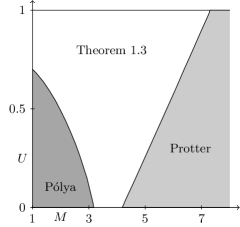
Figure 1. Theorem 1.3

On this, and all other figures, $M$ denotes the side with the middle length, and $U$ is equal to the difference between the length of the longest side and $M$. The shortest side is assumed to be $1$, hence $U\leq 1$. This gives a one-to-one mapping of all the triangles onto the infinite strip $[0,1)\times[1,\infty)$.

Next, we give some numerical results with Theorem 1.4 included. Since the bound involving the eigenvalues of circular sectors rely on the calculations of the zeros of the Bessel function, it is hard to compare to the other bounds. The numerical comparisons from Figure 2a show that this bound is better than the other bounds for almost all triangles.

One could also use a simplified sector based lower bound by just taking the smallest sector containing a given triangle. This gives the sector $S(\gamma N^{2}/2,\gamma)$ with the same angle as in Theorem 1.4, but larger radius. This is clearly worse than Theorem 1.4, but still gives a good bound as can be seen on Figure 2b.

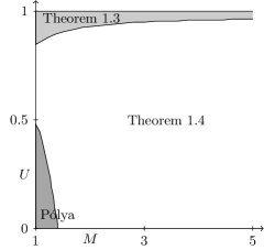
(a) Theorem 1.4

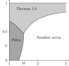
(b) Smallest sector containing a triangle

Figure 2. Sector-based bounds

We do note here that there is no best bound, although our new bounds together with Pólya’s give the best results depending on the triangle. We also see that symmetrization techniques (all bounds are consequences of certain symmetrization procedures) are very powerful and lead to very good lower bounds for the first eigenvalue of triangles.

It would be also interesting to see how far the bounds are from the exact values. We begin with a right isosceles triangle with arms of length $1$. The first eigenvalue is known in this case and it is equal to $5\pi^{2}$. The lower bounds results are given in Table 1a. Clearly, neither bound is particularly accurate, although Pólya’s bound and Theorem 1.4 are the closest.

The latter bound works best for “taller” triangles. Consider a right triangle with angle $\pi/6$ and hypotenuse $2$. Table 1b shows the values of the lower bounds for this triangle.

exact	49.348
Pólya (1.1)	45.5858
Freitas (1.15)	39.4784
Protter (1.14)	29.9958
Theorem 1.3	40.4654
Theorem 1.4	45.2255

(a) Right isosceles triangle

exact	30.7054
Pólya (1.1)	26.3189
Freitas (1.15)	23.0291
Protter (1.14)	19.0338
Theorem 1.3	23.9381
Theorem 1.4	29.8449

(b) Half of the equilateral triangle

Table 1. Triangles with known first eigenvalues

This time Theorem 1.4 gives a very close bound, while the others are not so accurate. The advantage of the sector bound is the biggest for very “tall” triangles. For an isosceles triangle with base $1$ and fixed arms we get Table 2. The exact values are not known, but the difference between the bounds given by Theorem 1.4 and the other bounds is clear.

	arm $2$	arm $4$
Pólya (1.1)	23.5404	11.4865
Freitas (1.15)	20.3972	12.4937
Protter (1.14)	17.0662	12.8437
Theorem 1.3	20.9906	12.9675
Theorem 1.4	27.0781	18.8754
Upper bound (6.1) in [S]	27.6695	18.9749

Table 2. Tall isosceles triangles

All these numerical results show that the lower bounds can be very accurate if the triangle is acute and almost isosceles (Pólya’s bound or Theorem 1.4). Unfortunately, neither bound is very good in the case of “wide” obtuse triangles. The values of the lower bounds for an isosceles triangle with base $1.95$ and arms $1$ are given in Table 3.

Pólya (1.1)	105.206
Freitas (1.15)	210.273
Protter (1.14)	205.698
Theorem 1.3	212.735
Theorem 1.4	185.161
Conjecture 1.2 in [S]
Lower bound	251.077
Upper bound	299.7

Table 3. Wide isosceles triangle

Clearly Freitas, Protter and Theorem 1.3 are the best in this case, but those values are not very accurate. In fact, neither bound allows us to prove the second part of the Theorem 1.1 in the case of obtuse triangles. Note that Conjecture 1.2 in [S] could provide a lower bound strong enough for this task. Theorems 2 and 5.1 in [F2] could also provide good enough bounds.

3. Symmetrization techniques

In this section we present various geometric transformations that decrease the first eigenvalue. The following subsections contain strict definitions of three different kinds of symmetrization. Here we just remark that the important common property of those transformations is that they are contractions on $W^{1,2}({{\mathbb{R}}^{d}})\cap C_{c}({{\mathbb{R}}^{d}})$ and isometries on $L^{2}({{\mathbb{R}}^{d}})$. Those properties, together with the minimax formula for the first Dirichlet eigenvalue, give $\lambda_{1}(\Omega)\geq\lambda_{1}(\Omega^{*})$. The most general reference for those results is [H].

3.1. Steiner Symmetrization

We start with the well known Steiner symmetrization (see for example [PS]*Note A or [H]*Chapter 2). Fix a line $l=\{ax+b:x\in{\mathbb{R}}\}$ where $a$ and $b$ are arbitrary points on the plane. Let $\{l_{t}\}_{t\in{\mathbb{R}}}$ be a family of lines perpendicular to $l$ such that for each $t$ the line $l_{t}$ passes through the point $at+b$. For an arbitrary domain $\Omega$ we define its Steiner symmetrization $\Omega^{*}$ with respect to $l$ as a convex domain symmetric with respect to $l$ and such that for every line $l_{t}$

(3.1) $$|\Omega^{*}\cap l_{t}|=|\Omega\cap l_{t}|,$$

where $|\cdot|$ denotes the $1$-dimensional Lebesgue measure.

Intuitively, we look at the cross-sections of $\Omega$ perpendicular to $l$ and we center them around $l$ (see Figure 3 for an example).

This procedure has many interesting properties (see [H, PS]). While the area remains fixed, the perimeter decreases and the inradius increases. But the most interesting property from our point of view is that the first eigenvalue of the Dirichlet Laplacian on $\Omega$ is bigger than that on $\Omega^{*}$. This basic property has been widely used in the proofs of many isoperimetric bounds for eigenvalues in many settings, see for example [AB, PS, H]. We will use this property to prove our results.

3.2. Continuous Steiner Symmetrization

The second type of symmetrization is the continuous Steiner symmetrization introduced by Pólya and Szegö in [PS]*Note B. Different versions of it have been studied by Solynin [S1] and Brock [B1, B2]. The difference in case of convex domains is only in the way of defining “continuity parameters”. The version studied in [B1, B2] is more general and it works even for not connected domains. We refer the reader to these three papers and to [H] for the properties of this transformation. Here we only give the definition valid for convex domains. As above we look at all the intervals $(a_{t},b_{t})$ which are the intersections of $\Omega$ with $l_{t}$. Let $(a_{t}^{\prime},b_{t}^{\prime})$ be the Steiner symmetrized interval. Let $a_{t}^{\alpha}=a_{t}+\alpha(a_{t}^{\prime}-a_{t})$ and $b_{t}^{\alpha}=b_{t}+\alpha(b_{t}^{\prime}-b_{t})$. Hence we are shifting the intersections with constant speed from their initial position to the fully symmetrized position. We define the continuous Steiner symmetrization $\Omega^{\alpha}$ of a domain $\Omega$ by

(3.2) $$\Omega^{\alpha}=\bigcup_{t\in{\mathbb{R}}}(a_{t}^{\alpha},b_{t}^{\alpha}).$$

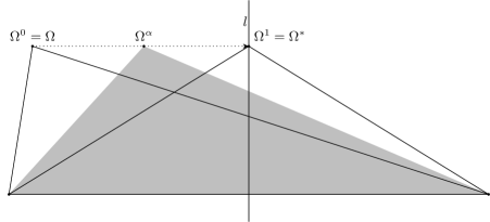
Figure 3. Continuous Steiner symmetrization

Figure 3 shows the action of continuous Steiner symmetrization on triangles. We can see that $\Omega^{0}=\Omega$ and $\Omega^{1}=\Omega^{*}$. The first eigenvalue of the domain $\Omega^{\alpha}$ is decreasing when $\alpha$ is increasing (see [B1, B2, H]) just like in the case of the classical Steiner symmetrization. Note that our “continuity parameter” $\alpha$ is related to the one in [H] by $1-\alpha=e^{-t}$.

3.3. Polarization

The last technique we want to introduce is called polarization. It was used in [Du] to prove general inequalities for capacities and eigenvalues. It has also been useful in studying other types of symmetrization (see [S1, BS]) and heat kernels for certain operators (see [Dr]). Let $l$ be an arbitrary line, $H_{1}$ and $H_{2}$ two halfspaces with boundary $l$. For $x\in H_{2}$ let $\bar{x}$ denote the reflection of $x$ with respect to $l$. Polarization of a domain $\Omega$ is defined pointwise by the following transformation

Definition 3.1.

The polarization of a set $\Omega$ with respect to $l$ is a set $\Omega^{P}$ with the following properties.

1. If $x\in\Omega\cap H_{1}$ then $x\in\Omega^{P}$.

2. If $x\in\Omega\cap H_{2}$ then $\bar{x}\in\Omega^{P}$.

3. If both $x$ and $\bar{x}$ are in $\Omega$, then both $x$ and $\bar{x}$ are in $\Omega^{P}$,

In essence, we reflect the set $\Omega$ with respect to $l$, the intersection of $\Omega$ with its reflection is in the polarized domain $\Omega^{P}$ and all other points of $H_{1}$ that are in either $\Omega$ or its reflection also belong to $\Omega^{P}$. Figure 4 shows a triangle, its reflection with respect to $l$ and the polarized domain (outlined polygon).

Figure 4. Polarization of sets

This simple procedure has many interesting monotonicity properties, among them is the monotonicity of the eigenvalues. For this, and many other properties we refer the reader to [BS, Dr] and to references in these papers.

4. The proofs of the lower bounds

Before we prove Theorems 1.3 and 1.4 let us present a one simple application of the continuous Steiner symmetrization. This and other kinds of symmetrization were introduced in Section 3.

Let $T$ be an acute isosceles triangle with area $A$ and arms of length $d$. Let $l$ be a line perpendicular to one of the arms and passing through the midpoint of this arm. If we apply the continuous Steiner symmetrization with respect to $l$ we get

Lemma 4.1.

Amongst triangles $T$ with diameter $d$ and area $A$, isosceles triangle with arms $d$ maximizes the first eigenvalue and isosceles triangle with base $d$ minimizes it (See Figure 3).

This simple result shows that upper bounds for the eigenvalues can also be obtained using symmetrization techniques. Using the largest circular sector contained in $T$ we can get very accurate upper bounds for the eigenvalues of triangles.

We can use polarization to give an alternate proof of (1.15). A very similar procedure, although more complicated, will be used later to prove Theorem 1.4. Let $T$ be an arbitrary triangle with the longest side of length $d$. First, we use the Steiner symmetrization with respect to a line perpendicular to the longest side. As a result we have an isosceles triangle $ABC$ with the base of length $d$.

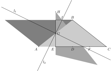
Figure 5. Freitas’s bound

The further construction is shown on Figure 5. We divide the longest side $AC$ into four equal parts. Then we construct the line $EH$ perpendicular to $AC$. Finally we construct the bisector $l_{1}$ of the angle $AGH$. We apply the polarization with respect to the line $l_{1}$. The darker triangle with vertex $H$ is the result of the reflection with respect to $l_{1}$. Note that we need the line $l_{1}$ to cut the side $AC$ between the points $E$ and $F$. If not, then we would not be able to symmetrize the other half of the triangle (the bisector would cut the sector $EG$, giving unnecessary reflections). Fortunately one can check that under the condition (2.7) this is always true.

Now we perform one more polarization with respect to the line $l_{2}$, which is the bisector of the angle $HIB$. As can be seen on Figure 5, the left side of the triangle has been changed into a rectangle.

If we repeat the procedure on the other side we get the rectangle with the base $EF$ and the height $BD$. But for a rectangle we have the following explicit formula for the first eigenvalue.

(4.1) $$\lambda_{1}|_{Rectangle}=\pi^{2}\left(a^{-2}+b^{-2}\right),$$

where $a$ and $b$ are the lengths of the sides. In our case the lengths are $|EF|=d/2$ and $|BD|=h$. This gives Freitas’s bound (1.15).

To get a sharper bound we need to symmetrize the triangle into a rectangle with a longer base and a shorter height. We start with the same Steiner symmetrization as before, That is, we symmetrize with respect to the line perpendicular to the longest side. Next, we perform one more Steiner symmetrization but with respect to the longest side. This gives a rhombus with diagonals of length $|CD|=h$ and $|EF|=h$ (see Figure 6).

Figure 6. Theorem 1.3

If we apply the Steiner symmetrization one more time but with respect to the height $DE$ of the rhombus, we obtain the rectangle with base $AC$ and height $DE$. Using Pythagorean theorem we find that $|AC|=\sqrt{d^{2}+h^{2}}/2$. Since the area $A$ of the triangle remains constant under symmetrization, we also have $|DE|=A/|AC|$. These, together with (4.1), give the proof of Theorem 1.3. Note, that the proof of Theorem 1.3 is actually easier than the proof of Freitas’s bound (1.15).

It remains to prove Theorem 1.4. Let us begin with a lemma.

Lemma 4.2.

Let $T$ be a triangle with the smallest angle $\gamma$. Let $T^{\prime}$ be a triangle with same area $A$ and same smallest angle $\gamma$ but with a smaller diameter. Then

(4.2) $$\lambda_{1}|_{T}\geq\lambda_{1}|_{T^{\prime}}.$$

Remark 4.3.

What this lemma essentially says is that we can continuously deform a triangle into an isosceles triangle, preserving the smallest angle and the area in such a way that the first eigenvalue will be decreasing. This immediately gives the first inequality in Theorem 1.4.

Proof.

This is perhaps the most complicated application of any symmetrization techniques. We have to apply a suitable sequence of polarizations to obtain the result. First, let $T_{\varepsilon}^{\prime}$ be a triangle similar to $T^{\prime}$ but with area $A+\varepsilon$. We will symmetrize $T$ into a set contained in $T_{\varepsilon}^{\prime}$. Then

(4.3) $$\lambda_{1}|_{T}\geq\lambda_{1}|_{T_{\varepsilon}^{\prime}}.$$

But when $\varepsilon\to 0$, the eigenvalue of $T_{\varepsilon}^{\prime}$ converges to the eigenvalue of $T^{\prime}$ and this ends the proof. Indeed, the triangles are similar hence we get the convergence due to scaling property of the eigenvalues.

Ideally, we would like to just define a sequence polarizations that folds $T$ inside $T^{\prime}_{\varepsilon}$. Unfortunately, it is virtually impossible to choose a correct line even for the first polarization. Each polarization must be with respect to a line cutting the longest and the shortest sides, but its exact position is not clear. The first line should be close to the vertex and the following lines should move away from the vertex. To give a precise position of each line we need to consider a temporary reversed sequence of transformations (very similar to the sequence of polarizations performed in the proof of 1.15). The first line in this reversed sequence (or the last line for polarization) is easy to define. Having this line we can get another, and so on. The precise construction is split into 4 steps.

Step 1: Definition of elementary transformation.

 

We start with two triangles $T=ABC$ and $T^{\prime}_{\varepsilon}=DBE$ such that $E$ is on the interval $BC$ and $A$ is on the interval $DB$. We also assume that the angle with vertex $B$ is the smallest in the triangle $T$ and that the area of $T^{\prime}_{\varepsilon}$ equals the area of $T$ plus $\varepsilon$. The triangles are shown on Figure 7a. Let $l_{1}$ be the bisector of the angle between the intervals $DE$ and $AC$. If we reflect $T$ with respect to this bisector we obtain another triangle $A^{\prime}B^{\prime}C^{\prime}$ shown on Figure 7b. Let $G$ be the intersection of $C^{\prime}B^{\prime}$ and $AC$.

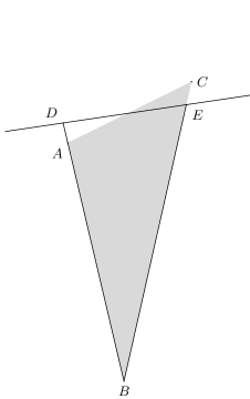
(a) $T$ and $T_{\varepsilon}^{\prime}$

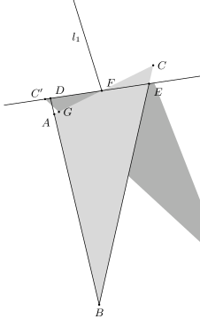
(b) the elementary transformation

Figure 7. Triangles $T=ABC$ and $T_{\varepsilon}^{\prime}=DBE$.

We define the elementary transformation of $T$ to be the polygon $ABEC^{\prime}G$. This construction is valid due to two conditions. The first, the area of $DBE$ is bigger than the area of $ABC$. The second, the angle $\angle ACB$ is smaller than the angle $\angle EDB$. Those two conditions guarantee that the bisector cuts the sides $AC$ and $BC$ and not the side $AB$ and validates the construction of the elementary transformation.

The same transformation can be applied to more general domains. For example any domain contained in an infinite cone $ACB$ with vertex at $C$. We will need this observation later on.

Notice also that the elementary transformation is equivalent to polarization with respect to the bisector for any domain containing $ABC$ as long as: the intersection of this domain with the bisector is the same as the intersection of $ABC$ with the bisector, the new part (triangle $C^{\prime}GF$ in the case above) does not intersect the domain. In particular we could take a domain consisting of $ABC$ and any subset of a half-plane disjoint with $ABC$ and with boundary containing $AB$ unless this domain intersects the bisector or $C^{\prime}GF$. We also do not need $C^{\prime}GF$ to be a triangle, it is enough that this set does not intersect the domain.

Step 2: Sequence of elementary transformations.

 

Now we want to describe a sequence of elementary transformations that changes $T=ABC$ into a subset of $T^{\prime}_{\varepsilon}=DBE$.

The first transformation is described in Step 1. It is clear that the area of $ADF$ is bigger than the area of $C^{\prime}GF$. We have

(4.4) $$\angle GC^{\prime}F=\angle ACB<\angle ACB+\angle ABC=\angle DAF.$$

Therefore the second elementary transformation can be applied to triangles $C^{\prime}GF$ and $ADF$ (see Figure 8a). Here we completely disregard the presence of the quadrilateral $AFEB$.

This elementary transformation introduces a new triangular piece that may intersect the triangle $ABC$ near vertex $A$ (see Figure 8b). The intersection means that the elementary transformation is not equivalent to the polarization of $ABEC^{\prime}G$ (we did not care about the quadrilateral $AFEB$ while making a transformation). This intersection will not occur if the triangle $ADF$ is large enough to fit the triangle $C^{\prime}GF$ inside. It would follow that the second elementary transformation is also equivalent to polarization. In such a case the construction of the sequence of transformations would be finished.

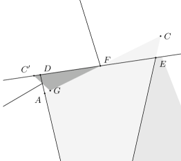
(a) bisector

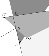
(b) transformation and intersection

Figure 8. The second transformation

If the intersection occurs, we apply another elementary transformation to the triangle introduced during the previous transformation and to the difference between the triangles considered for the previous transformation (triangle $AGH$). Here we again disregard the presence of other part of the domain. The third elementary transformation is shown on Figure 9. To validate this step we need to check that the angle $\angle AGH$ is bigger than the angle $\angle ACB$. Indeed, it is equal to the angle $\angle GC^{\prime}F$($=\angle ACB$) plus the angle $\angle C^{\prime}FG$.

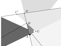
Figure 9. The third transformation

If the newly introduced triangular piece does not intersect the already obtained domain (as on Figure 9), the construction in finished. If it does, we apply another elementary transformation (or as many elementary transformations as needed) to fully “fold” the triangle $ABC$ inside of the triangle $DBE$. The final subset of $DBE$ that has the same area as $ABC$ will have a spiral-like pattern of triangular pieces introduced by consecutive elementary transformations. First we need to show that this process is finite. Later we need to modify the procedure to get a sequence of valid polarizations. In particular we need to avoid self-intersecting that happens at every stage.

Step 3: Finiteness of the construction.

 

To estimate the area of the subset of $ADF$ that is covered using three consecutive elementary transformations, we shift the triangular pieces obtained each time so that the angle equal to the angle $ACB$ has a vertex at $D$, $A$ and $F$ respectively (after the second, third and fourth elementary transformation). The triangle $A^{\prime}B^{\prime}C^{\prime}$ is shifted so that vertex $C^{\prime}$ moves to $D$, $G$ moves to $F^{\prime}$ and the angle $\angle FDF^{\prime}$ is equal to the angle $\angle ACB$. We do the same with other triangles. See Figure 10 for the picture of the shifted pieces. This decreases the covered area, but does not change the angles between any of the lines.

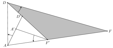
Figure 10. Covering using the angle $ACB$ (arrow)

We have

(4.5) $$\angle A^{\prime}F^{\prime}D^{\prime}+\angle AF^{\prime}A^{\prime}=\angle F^{\prime}DF+\angle F^{\prime}FD.$$

This implies that the angle $\angle A^{\prime}F^{\prime}D^{\prime}$ equals the angle $\angle AFD$. Similarly we show that other angles of the triangles $AFD$ and $A^{\prime}F^{\prime}D^{\prime}$ are also equal. This means that three elementary transformations reduce the uncovered part to a triangle similar to $AFD$. The size of this triangle is not bigger than the size of $A^{\prime}D^{\prime}F^{\prime}$. Therefore the area of the uncovered part is shrinking at a constant rate. Due to the difference in the area of $T^{\prime}_{\varepsilon}$ and $T$ the procedure must end as soon as the area of the uncovered part is smaller than $\varepsilon$.

Step 4: Sequence of polarizations.

 

The presence of intersections in the second and all consecutive elementary transformations stops us from using the sequence of elementary transformations as a sequence of polarizations. To fix this problem we consider the same sequence of transformations, but in the reverse order. Each elementary transformation was applied to a triangle that is a part of the reflection of the triangle $ABC$. Therefore we can treat those elementary transformations as a transformations on $ABC$.

As we remarked in Step 1 such transformations are equivalent to polarizations. We use the reflection lines used by the elementary transformations to produce polarizations. Figures 11a and 11b show the domain after the first two polarizations or the last two elementary transformations (outlined sets). The construction from Step 2 ensures that the triangular pieces introduced at every step have no intersection with the reflection lines. We also avoid self-intersecting since the triangular pieces are introduced in the reverse order. This means that we have a sequence of valid polarizations.

The last polarization (the first elementary transformation) fits the whole domain inside $T_{\varepsilon}^{\prime}=DBE$ (see Figure 12). If the sequence is longer than on the example, we proceed in the same manner, building the spiral-like structure starting from the smallest inner triangle.

This proves that for arbitrary $\varepsilon>0$ there exists a finite sequence of polarizations, which transforms $T$ into a subset of $T_{\varepsilon}^{\prime}$.

This sequence of polarizations can be constructed even for domains consisting of triangle $ABC$ and any set contained in the half-plane with boundary $AB$ and disjoint with $ABC$.

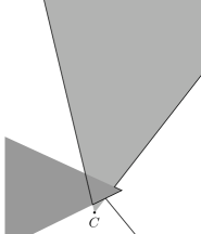
(a) The first polarization (the third transformation)

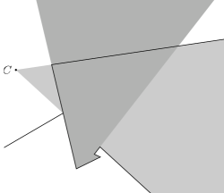
(b) The second polarization (the second transformation)

Figure 11. Reversed steps

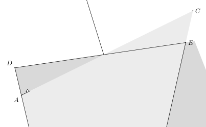
Figure 12. The third polarization (the first transformation)

∎

Remark 4.4.

The same proof as for Lemma 4.2 works for any domain contained in an infinite cone $ACB$ and containing $T$.

Lemma 4.5.

Let $\Omega$ be a kite, that is a quadrilateral symmetric with respect to the longer diagonal and with perpendicular diagonals. Assume also that the length of the longer diagonal is smaller than the length of one of the sides. Given the fixed area and the smallest angle, the first eigenvalue is decreasing with the diameter. In particular, an isosceles triangle has a maximal first eigenvalue among kites with fixed area and the smallest angle, the kite consisting of two isosceles triangles has minimal first eigenvalue.

Proof.

We can split an isosceles triangle $ABC$ into two right triangles and use Lemma 4.2 and the remark above to symmetrize any one of those right triangles (for example $DBC$ on Figure 13a). Furthermore, we can perform all but the last polarization on both right triangles (Figure 13b shows the domain at this stage of construction). Finally we can perform the last polarizations to get the quadrilateral with vertex $E$. The last transformations are indeed polarizations since the bisectors are cutting the line $BD$ below the point $B$ (certainly not between points $D$ and $E$).

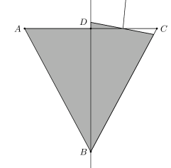
(a) one-sided symmetrization

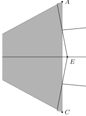
(b) two-sided symmetrization before the last step

Figure 13. Isosceles triangle

∎

The proof of the second inequality in Theorem 1.4 requires a repeated use of the above results. As before we take a slightly larger sector $S(A+\varepsilon,\gamma)$ instead of $S(A,\gamma)$. We need to transform the isosceles triangle $I(A,\gamma)$ into a subset of $S(A+\varepsilon,\gamma)$. Using Lemma 4.5 we can symmetrize the triangle $ABC$ into a quadrilateral (see Figure 14a) with longer diagonal equal to the radius of the circular sector $S(A+\varepsilon,\gamma)$.

Now we divide both halves of the quadrilateral into $N$ (to be chosen later) parts by dividing the angle with vertex $B$ into equal parts (see Figure 14b).

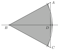
(a) quadrilateral

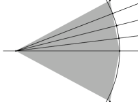
(b) subdivisions

Figure 14. Symmetrized isosceles triangle

We work on each half separately. Consider a triangle formed by all but the inner most part. We use Remark 4.4 to symmetrize this triangle into a “more isosceles” triangle with one vertex on an intersection of a circular part and the innermost line. This makes the part outside of the circular sector smaller. Now we repeat this using decreased number of parts. The picture after two steps is shown on Figure 15. By choosing a large enough $N$ and performing all steps we can fit the whole half of the quadrilateral inside of the circular sector.

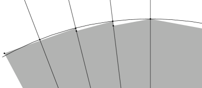
Figure 15. Intermediate stage of construction

This ends the proof of the second inequality in the Theorem 1.4. The last thing to prove is the monotonicity property for the isosceles triangles. Here we need to apply the continuous symmetrization to obtain the result. Suppose that we start with the isosceles triangle $I(A,\gamma)$ with the vertex angle smaller than $\pi/3$. We want to show that if we increase the angle to $\pi/3\geq\gamma^{\prime}>\gamma$ while the area remains fixed, then the first eigenvalue decreases. First, we apply the continuous Steiner symmetrization with respect to the line perpendicular to one of the arms. The length of the base increases, and its maximal length is obtained when we reach the full Steiner symmetrization. Compare with Figure 3 where the shortest side of $\Omega^{\alpha}$ increases with $\alpha$.

If this maximum is smaller than the base of $I(A,\gamma^{\prime})$, we use the Steiner symmetrization to get an isosceles triangle with the angle $\gamma^{\prime\prime}$ between $\gamma$ and $\gamma^{\prime}$ and the base equal to this maximum. We can repeat the above procedure on the triangle $I(A,\gamma^{\prime\prime})$.

On the other hand, if the maximum is bigger than the base of $I(A,\gamma^{\prime})$, then we can stop the continuous Steiner symmetrization at the time when the length of the enlarged base of $I(A,\gamma)$ is equal to the base of $I(A,\gamma^{\prime})$ (on Figure 3 we choose $\alpha$ such that the shortest side is equal to the base of $I(A,\gamma^{\prime})$. Now, the Steiner symmetrization with respect to the base gives an isosceles triangle with the base equal to the base of $I(A,\gamma^{\prime})$. This implies that it must be equal to $I(A,\gamma^{\prime})$.

Suppose that the vertex angle $\gamma>\pi/3$. The same procedure as above shortens the base in this case. The same argument applies, but with maximum replaced with minimum. This ends the proof of the Theorem 1.4.

5. The proofs of the upper bounds

In this section we prove Theorem 1.1. The approach we take is based on variational bounds for the second eigenvalue. This approach is a modification of the similar method used in [S]. We start with the minimax formula for the second eigenvalue.

(5.1) $$\lambda_{2}|_{D}=\inf_{f_{1},f_{2}}\sup_{\alpha\in{\mathbb{R}}}\frac{\int_{D}|\nabla(f_{1}+\alpha f_{2})|^{2}}{\int_{D}|f_{1}+\alpha f_{2}|^{2}},$$

where $f_{1},f_{2}\in H^{1}_{0}(D)$ are linearly independent. This formula is a special case of the general minimax formula for an arbitrary eigenvalue (see e.g. [Da]). As in [S], we will use known eigenfunctions for equilateral or right triangles to obtain test functions for arbitrary triangles.

Consider the equilateral triangle $T_{e}$ with vertices $(0,0)$, $(1,0)$ and $(1/2,\sqrt{3}/2)$. The complete set of eigenfunctions is well known. For the exact formulas for these eigenfunctions we refer the reader to [P, M]. In particular, [M] gives the simple formulas that we will use in this paper. Let

(5.2) $$z=\frac{\pi}{3}(2x-1),$$

(5.3) $$t=\pi\left(1-\frac{2}{\sqrt{3}}y\right).$$

The first eigenfunction is given by

(5.4) $$\varphi_{1}(x,y)=(\cos(3z)-\cos(t))\sin(t).$$

The second eigenvalue has multiplicity two. We will follow the notation from [M] to name these eigenfunctions. All eigenfunctions can be divided into two kinds: symmetric and antisymmetric. The first will be denoted by $S$ followed by two numbers identifying the eigenfunction. The second by $A$ also followed by two numbers. For the details about this notation we refer the reader to [M]. The two eigenfunctions belonging to the second eigenvalue are

(5.5) $$\varphi_{S21}(x)=\cos(4z)\sin(2t)+\cos(5z)\sin(t)-\cos(z)\sin(3t),$$

(5.6) $$\varphi_{A21}(x)=\sin(4z)\sin(2t)+\sin(5z)\sin(t)-\sin(z)\sin(3t).$$

Let $T$ be an arbitrary triangle. We can assume that one side of this triangle is equal to the segment from $(0,0)$ to $(1,0)$, and that the last vertex $(u,v)$ is in the upper halfspace. Then, there exists a unique linear transformation $L$ from $T$ onto $T_{e}$. As in [S], we will compose $L$ with the eigenfunctions of $T_{e}$ to obtain suitable test functions for $T$.

Using formula (5.1) we obtain an upper bound

(5.7) $$\lambda_{2}|_{T}\leq\sup_{\alpha\in{\mathbb{R}}}\frac{\int_{T}|\nabla(g_{\alpha}\circ L)|^{2}}{\int_{T}|g_{\alpha}\circ L|^{2}},$$

where $g_{\alpha}$ is a linear combination of two known eigenfunctions.

As the first two test functions we can take

(5.8) $$g^{1}_{\alpha}(x,y)=\varphi_{S21}(x,y)+\alpha\varphi_{S11}(x,y),$$

(5.9) $$g^{2}_{\alpha}(x,y)=\varphi_{A21}(x,y)+\alpha\varphi_{S11}(x,y).$$

If the triangle $T$ is almost equilateral, we can expect that its eigenvalues and eigenfunctions are similar to the eigenvalues and eigenfunctions of $T_{e}$. Also, the linear transformation $L$ should not perturb the bound (5.7) significantly. Therefore, we can expect that for almost equilateral triangles this should be a good upper bound for $\lambda_{2}|_{T}$.

Notice that the linear combinations in (5.8) and (5.9) consist of two orthogonal functions. Hence the second norm of this combination is just the sum of the second norms. Therefore

(5.10) $$\sup_{\alpha\in{\mathbb{R}}}\frac{\int_{T}|\nabla(g_{\alpha}\circ L)|^{2}}{\int_{T}|g_{\alpha}\circ L|^{2}}=\frac{a\alpha^{2}+b\alpha+c}{e\alpha^{2}+f},$$

where $a$,$c$,$e$,$f$ are strictly positive. This rational function has a limit $a/e$, as $\alpha\to\pm\infty$. By taking its derivative we can also find the critical points

(5.11) $$\alpha_{1}=\frac{1}{bd}\left(af-ce-\frac{1}{2}\sqrt{4b^{2}ef+(2af-2ce)^{2}}\right),$$

(5.12) $$\alpha_{2}=\frac{1}{bd}\left(af-ce+\frac{1}{2}\sqrt{4b^{2}ef+(2af-2ce)^{2}}\right).$$

If we evaluate the function at those points and simplify, we get

(5.13) $$C_{1}=\frac{1}{2ef}\left(af+ce-\frac{1}{2}\sqrt{4b^{2}ef+(2af-2ce)^{2}}\right),$$

(5.14) $$C_{2}=\frac{1}{2ef}\left(af+ce+\frac{1}{2}\sqrt{4b^{2}ef+(2af-2ce)^{2}}\right).$$

The expression under the root is clearly nonnegative. It is zero if $b=0$ and $af=ce$. In such case $C_{1}=C_{2}=a/e$, hence the maximum is $a/e$. If the expression under the root is positive, then we have two distinct critical points, and $C_{2}>C_{1}$. This means that this rational function has an absolute maximum $C_{2}$ and absolute minimum $C_{1}$.

This leads to a new bound for the eigenvalue

(5.15) $$\lambda_{2}|_{T}\leq C_{2}=\frac{1}{2ef}\left(af+ce+\frac{1}{2}\sqrt{4b^{2}ef+(2af-2ce)^{2}}\right).$$

To finish the proof of Theorem 1.1 we need to use one of the lower bounds for the first eigenvalue. Due to the simple form of the bound, we will use Freitas’s result (1.15). To prove the first bound in Theorem 1.1 we need to show that

(5.16) $$((\ref{upsimple})-(\ref{freitas}))R^{2}\leq\frac{16\pi^{2}}{27},$$

where we have used the reference number of the equation for the value given by it. The number on the right side of the inequality is the exact value obtained for the equilateral triangle.

The second bound will be proved if we can show that

(5.17) $$\frac{(\ref{upsimple})}{(\ref{tA})}\leq\frac{7}{3}.$$

Notice that this time we use Pólya’s isoperimetric bound (1.1).

Let us begin with the proof of (5.16). We first use $g^{1}_{\alpha}$ as a test function. The expressions (5.15) and (1.15) can be written in terms of the vertices of the triangle $T$. But we assumed that the vertices are $(0,0)$, $(1,0)$ and $(u,v)$. We denote the lengths of the sides of the triangle by $1$, $M=\sqrt{u^{2}+v^{2}}$, $N=\sqrt{(1-u)^{2}+v^{2}}$ and we can assume that $N\geq M\geq 1$. Then the bound (5.16) (in terms of the lengths of the sides) is equivalent to

$$0\geq-1612800N^{2}(1+M+N)^{2}\pi^{2}+27\Bigl{\{}-413343N^{2}V$$

(5.18) $$+11200(9(M^{2}-1)^{2}+2(M^{2}+1)N^{2}+20N^{4})\pi^{2}$$

$$+N^{2}\sqrt{655128046899V^{2}-74071065600VW\pi^{2}+8028160000W^{2}\pi^{4}}\Bigr{\}},$$

where $V=M^{2}+N^{2}-2$ and $W=M^{2}+N^{2}+1$.

The expression is quite complicated since the integrals of the function $g^{1}_{\alpha}$ are very cumbersome to calculate. This task could be accomplished by hand since this function is just a sum of the products of the trigonometric functions. However, symbolic calculations in Mathematica are used to obtain this expression in a short time. The script performing all the calculations from this section is included in the last section.

One can check numerically where this inequality is true. If we put $U=N-M$ then the set of all possible triangles can be characterized by $U\in[0,1)$ and $M\geq 1$. The dark part of Figure 16 corresponds to those triangles for which the inequality is valid.

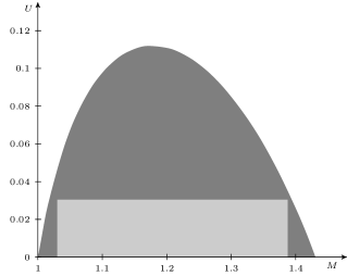
Figure 16. Bound 1/Case 1: The numerical solution

It is clear that not all triangles can be handled this way. Hence we have to use more then one test function, and divide all triangles into subregions of $U\in[0,1)$ and $M\geq 1$. We will define other test functions at the end of the section.

We now prove inequality (5.18) on the gray rectangle shown in Figure 16. More precisely we take $U\in[0,0.03]$ and $M\in[1.03,1.39]$.

The inequality (5.18) can be written as

(5.19) $$P(N,M)+Q(N,M)\sqrt{R(N,M)}\leq 0,$$

where $P$, $Q$ and $R$ are polynomials in $N$ and $M$. It will be proved, if we can show that

(5.20) $$P(N,M)\leq 0,$$

(5.21) $$Q^{2}(N,M)R(N,M)-P^{2}(M,N)\leq 0.$$

This is a system of polynomial inequalities. Unfortunately the degrees of those polynomials are 4 and 8 in each variable. Therefore there is almost no hope to solve this system using any conventional method.

Instead, we developed an algorithm for solving such polynomial inequalities on rectangles. The next section contains a detailed description of this algorithm and the proof of its correctness. It turned out that in our case this method gives the proof of the inequality for any test function we tried.

To finish the proof of the first part of Theorem 1.1 we need to define the other test functions and rectangles for each corresponding inequality.

We already have two test functions (5.8) and (5.9) that came from the equilateral triangle. We can also use the first two eigenfunctions of the half of the equilateral triangle. That is, of the right triangle with angle $\pi/6$. Its eigenfunctions are certain antisymmetric eigenfunctions of the equilateral triangle. Hence, we get the third test function

(5.22) $$g^{3}_{\alpha}(x,y)=\varphi_{A31}(x,y)+\alpha\varphi_{A21}(x,y),$$

where (using notation (5.2) and (5.3))

(5.23) $$\varphi_{A31}(x,y)=\sin{5z}\sin{3t}-\sin{2z}\sin{4t}-\sin{7z}\sin{t}.$$

In this case we also need to get a new linear transformation $L^{\prime}$ that transforms the given triangle into the right triangle.

The last case when all eigenfunctions are known is the right isosceles triangle. Since this triangle is “half” of a square, its eigenfunctions are equal to eigenfunctions of the square with diagonal nodal lines. We get

(5.24) $$g^{4}_{\alpha}(x,y)=\phi_{2}(x,y)+\alpha\phi_{1}(x,y),$$

where

(5.25) $$\phi_{1}(x,y)=\sin{2\pi x}\sin{\pi y}+\sin{\pi x}\sin{2\pi y},$$

(5.26) $$\phi_{2}(x,y)=\sin{3\pi x}\sin{\pi y}-\sin{\pi x}\sin{3\pi y}.$$

We can also mix the eigenfunctions from the different triangles provided we use appropriate linear transformation for each of them. In this manner we obtain the last (fifth) case needed to prove the theorem by taking $g^{1}_{\alpha}(x,y)$ and $\frac{1}{2}\phi_{2}(x,y)$.

Each of the five cases requires a rectangle on which we can prove the bound. We take

1. $U\in[0,0.03]$, $M\in[1.03,1.39]$,

2. $U\in[0,0.2]$, $M\in[1,1.03]$,

3. $U\in[0,1)$, $M\in[1.39,\infty)$,

4. $U\in[0.2,1)$, $M\in[1,1.39]$,

5. $U\in[0.03,0.2]$, $M\in[1.03,1.39]$.

Notice that these rectangles exactly cover the infinite strip $[0,1)\times[1,\infty)$. Since the sides of the triangle are $N\geq M\geq 1$ and $U=N-M$, the strip includes all possible combinations of lengths of the sides.

The proof in cases (3)-(5) is exactly the same as in case (1). Additional step has to be performed in case (2). Consider a triangle $T^{\prime}$ similar to $T$ with sides $1$, $N^{\prime}=M/N$, $M^{\prime}=1/N$. We have $1\geq N^{\prime}\geq M^{\prime}$. Consider inequality (5.16) for $T^{\prime}$. Note that the diameter of $T^{\prime}$ used in (1.15) is now $1$ ($N$ in other cases). Just like before we get an expression similar to (5.18) but involving $N^{\prime}$ and $M^{\prime}$. After a change of variable $M^{\prime}\to N^{\prime}-M^{\prime}+1$ and $N^{\prime}\to 1-U^{\prime}$ we can apply our algorithm with a rectangle given in case (2). This proves the bound (5.16) for $T^{\prime}$, and hence for $T$ since the bound is invariant under scaling.

We need to check that the transformation

(5.27) $$\frac{M}{M+U}=1-U^{\prime},$$

(5.28) $$\frac{1}{M+U}=2-U^{\prime}-M^{\prime},$$

changes the rectangle $U\in[0,0.2)$, $M\in[1,1.03)$ into a subset of the same rectangle in primed variables. From the first equation we get

(5.29) $$0\leq U^{\prime}=1-\frac{M}{M+U}\leq 1-\frac{1}{1.23}<0.19.$$

From the second equation

(5.30) $$1\leq M^{\prime}=\frac{M-1}{M+U}+1\leq\frac{M-1}{M}+1=2-\frac{1}{M}\leq 2-\frac{1}{1.03}<1.0292.$$

This ends the proof of the first part of Theorem 1.1. The second part requires an additional argument. We still need to use test functions $g^{1}_{\alpha}(x,y)$ through $g^{5}_{\alpha}(x,y)$ on the following rectangles

1. $U\in[0,0.09]$, $M\in[1,1.37]$;

2. not needed;

3. $U\in[0,0.42]$, $M\in[1.37,2.05]$;

4. $U\in[0.09,0.2]$, $M\in[1,1.37]$;

5. $U\in[0.2,0.42]$, $M\in[1,1.37]$.

Notice that in each case $U\leq 0.42$. Since the triangles are acute we have $N^{2}\leq M^{2}+1$, hence $U\leq\sqrt{2}-1$. Also, all these rectangles cover only the cases with $M\leq 2.05$.

Therefore we need a circular sector type–bound similar to the one in [S]. We use the sector bound from Theorem 1.4 for the first eigenvalue and the upper bound for the second eigenvalue based on the biggest circular sector contained in the given triangle. Suppose that we have an acute triangle with area $A$ and smallest angle $\gamma$. Let $N\geq M\geq 2.05$ be the two longest sides. Since the triangle is acute, the largest sector contained in the triangle has the radius equal to the longest altitude $H$. We get

(5.31) $$\left.\frac{\lambda_{2}}{\lambda_{1}}\right|_{Triangle}\leq\frac{\lambda_{2}|_{S(\gamma H^{2}/2,\gamma)}}{\lambda_{1}|_{S(A,\gamma)}}.$$

This bound is certainly good enough, but it is hard to deal with due to the complicated formula for the radius of the circular sector $S(A,\gamma)$. Therefore we have to rely on the weaker bound

(5.32) $$\left.\frac{\lambda_{2}}{\lambda_{1}}\right|_{Triangle}\leq\frac{\lambda_{2}|_{S(\gamma H^{2}/2,\gamma)}}{\lambda_{1}|_{S(\gamma MN/2,\gamma)}}.$$

This bound also follows from Theorem 1.4 by taking the smallest sector containing the isosceles triangle $I(A,\gamma)$ (first inequality in Theorem 1.4) with the arms of the length $\sqrt{MN}$.

The eigenvalues of the circular sectors are given in terms of the zeros $j_{v,n}$ of the Bessel function of index $v$. Here $n$ indicates $n$-th smallest zero. We have

(5.33) $$\lambda_{1}|_{S(\gamma R^{2}/2,\gamma)}=R^{-2}j_{\pi/\gamma,1}^{2},$$

(5.34) $$\lambda_{2}|_{S(\gamma H^{2}/2,\gamma)}\leq\lambda_{12}(Sector)=R^{-2}j_{\pi/\gamma,2}^{2}.$$

Notice that we only have the inequality for the second eigenvalue due to the presence of another eigenfunction $\lambda_{21}(Sector)$. This eigenvalue may be smaller than $\lambda_{12}(Sector)$.

We can use the bounds for the zeros of the Bessel functions proved in [QW]. That is,

(5.35) $$v-\frac{a_{k}}{\sqrt[3]{2}}\sqrt[3]{v}<j_{v,k}<v-\frac{a_{k}}{\sqrt[3]{2}}\sqrt[3]{v}+\frac{3}{20}a_{k}^{2}\frac{\sqrt[3]{2}}{\sqrt[3]{v}},$$

where $a_{k}$ are zeros of the Airy function with $a_{1}\approx-2.3381$ and $a_{2}\approx-4.0879$.

Using the last two facts we obtain

(5.36) $$\begin{split}\left.\frac{\lambda_{2}}{\lambda_{1}}\right|_{Triangle}&\leq\frac{NM}{H^{2}}\left(\frac{x^{3}-\frac{a_{2}}{\sqrt[3]{2}}x+\frac{3}{20}a_{2}^{2}\frac{\sqrt[3]{2}}{x}}{x^{3}-\frac{a_{1}}{\sqrt[3]{2}}{x}}\right)^{2}\\ &=\frac{NM}{H^{2}}\left(\frac{1-\frac{a_{2}}{\sqrt[3]{2}}x^{-2}+\frac{3}{20}a_{2}^{2}\frac{\sqrt[3]{2}}{x^{4}}}{1-\frac{a_{1}}{\sqrt[3]{2}}{x^{-2}}}\right)^{2},\end{split}$$

where $x=(\pi/\gamma)^{1/3}$. Note that for acute triangles we have $N^{2}\leq M^{2}+1$. We need to consider two cases based on the length of $H$. First assume that $H^{2}\geq M^{2}-1/16$. This is equivalent to the condition that the altitude $H$ divides the shortest side (with the length $1$) into two parts with one of them not longer than $1/4$. Using the inequality $N^{2}\leq M^{2}+1$, we obtain

(5.37) $$\frac{NM}{H^{2}}\leq\frac{M\sqrt{M^{2}+1}}{M^{2}-\frac{1}{16}}=\sqrt{1+M^{-2}}\left(1-\frac{1}{16M^{2}}\right)^{-1}=:z_{1}(M).$$

If $M^{2}-1/4\leq H^{2}\leq M^{2}-1/16$ then the altitude $H$ divides the shortest side into two parts, one of length $\delta$ satisfying $1/4<\delta<1/2$ and the other of length $1-\delta$. Then

(5.38) $$N^{2}=H^{2}+(1-\delta)^{2}=M^{2}-\delta^{2}+(1-\delta)^{2}=M^{2}+1-2\delta\leq M^{2}+\frac{1}{2}.$$

This gives

(5.39) $$\frac{NM}{H^{2}}\leq\frac{M\sqrt{M^{2}+\frac{1}{2}}}{M^{2}-\frac{1}{4}}=\sqrt{1+\frac{1}{2M^{2}}}\left(1-\frac{1}{4M^{2}}\right)^{-1}=:z_{2}(M).$$

Let $z(M)=\max\left\{z_{1}(M),z_{2}(M)\right\}$. Note that $z(M)$ is decreasing since both $z_{1}(M)$ and $z_{2}(M)$ are decreasing. Making the substitution $y=x^{-2}$ we get

(5.40) $$\begin{split}\left.\frac{\lambda_{2}}{\lambda_{1}}\right|_{Triangle}&\leq z(M)\left(\frac{1-\frac{a_{2}}{\sqrt[3]{2}}y+\frac{3\sqrt[3]{2}}{20}a_{2}^{2}y^{2}}{1-\frac{a_{1}}{\sqrt[3]{2}}y}\right)^{2}\\ &=z(M)\left(c_{1}+c_{2}y+\frac{c_{3}}{1+c_{4}y}\right)^{2},\end{split}$$

where the constants $c_{i}$ satisfy

(5.41) $$c_{1}=\frac{(10a_{1}-3a_{2})a_{2}}{10a_{1}^{2}}\approx 0.83133>0,$$

(5.42) $$c_{2}=-\frac{3a_{2}^{2}}{10\sqrt[3]{2}a_{1}}\approx 1.70183>0,$$

(5.43) $$c_{3}=\frac{10a_{1}^{2}-10a_{1}a_{2}+3a_{2}^{2}}{10a_{1}^{2}}\approx 0.16867>0,$$

(5.44) $$c_{4}=-\frac{a_{1}}{\sqrt[3]{2}}\approx 1.85575>0.$$

We want to show that the right hand side of (5.40) is decreasing with $M$ (note that $y$ also depends on $M$ since it depends on $\gamma$). First we can show that this expression is increasing with $y$ for a fixed $M$. Indeed, the derivative with respect to $y$ is $c_{2}-\frac{c_{3}}{(1+c_{4}y)^{2}}$ and it is positive for $y>0$ due to the condition $c_{2}>c_{3}$. This means that the expression is also increasing in $\gamma$ since $y=(\pi/\gamma)^{-2/3}$. If we fix $M$, then from all triangles with sides $1$, $M\geq 1$, $N\geq M$, the isosceles triangle ($M=N$) has the biggest angle $\gamma$. In this case $\cos\gamma=1-\frac{1}{2M^{2}}$. As a result we get an upper bound for the ratio of the first two eigenvalues in terms of $M$. That is, we have

(5.45) $$\left.\frac{\lambda_{2}}{\lambda_{1}}\right|_{Triangle}\leq z(M)\left(c_{1}+c_{2}y_{M}+\frac{c_{3}}{1+c_{4}y_{M}}\right)^{2},$$

with $y_{M}=(\arccos(1-(2M^{2})^{-1})/\pi)^{2/3}$. But $y_{M}$ and $z(M)$ are decreasing with $M$, hence the right hand side is decreasing with $M$. To finish the proof we just need to check that this is smaller than $7/3$, as required in (5.17), for $M=2.05$ (we get $\approx 2.3285<7/3$). This ends the proof of Theorem 1.1.

6. An algorithm for polynomial inequalities

This section gives the algorithm for proving polynomial inequalities in two variables with arbitrary degrees. The domain we deal with is a rectangle. The proof of the correctness is also given.

Suppose that we have an inequality

(6.1) $$P(x,y)=\sum_{i=0}^{n}\sum_{j=0}^{m}c_{i,j}x^{i}y^{j}\leq 0,$$

for $x\in(0,a)$ and $y\in(0,b)$. Any other rectangle can be shifted to the origin, hence reducing the problem to this case.

The idea behind the algorithm is very simple. For any monomial

(6.2) $$c_{i,j}x^{i}y^{j}\leq c_{i,j}\min\{ax^{i-1}y^{j},bx^{i}y^{i-1}\},\mbox{ if }c_{i,j}>0,$$

(6.3) $$c_{i,j}x^{i}y^{j}\leq c_{i,j}\max\{a^{-1}x^{i+1}y^{j},b^{-1}x^{i}y^{i+1}\},\mbox{ if }c_{i,j}<0.$$

We can use this simple observation to reduce the number of positive coefficients in $P(x,y)$. Clearly, if we apply any of the above inequalities finite number of times on any of the monomials in P(x,y), we obtain an upper bound for $P(x,y)$. If we can reduce the whole polynomial to 0, we proved inequality (6.1).

We need to describe a sequence of reductions, that leads to a constant or to a polynomial with only positive coefficients. If we get at least one strictly positive coefficient we cannot say that inequality is false, since we are using an upper bound for $P(x,y)$. Thus, the algorithm does not always work although it is possible to generalize it. In case of the false answer we can divide the rectangle into four identical sub–rectangles, and rerun the algorithm on each of them. As long as the inequality $P(x,y)\leq 0$ is strict, this recursive procedure should give the proof.

It is worth noting that for 8 out of the 9 polynomials we have in the previous section this method works on the whole rectangle (without sub–dividing). In the case of the third test function in the second part of Theorem 1.1 we need to split the given rectangle into halves. The gray rectangle on Figure 16 in the previous section is almost as big as possible given that the inequality is true only for the dark points. Hence the method works very well in this case. By running the script from the last section one can see that in all other cases the method is also very efficient.

Now we will define the optimal sequence of reductions. The only way to reduce a positive coefficient is by lowering the power of one of the variables (using (6.2)). Similarly, to reduce a negative coefficient we have to increase one of the powers (using (6.3)). Each time, two of the coefficients combine giving a new, possibly negative coefficient. Write

(6.4) $$P(x,y)=\sum_{i=0}^{n}x^{i}Q_{i}(y),$$

where

(6.5) $$Q_{i}(y)=\sum_{j=0}^{m}c_{i,j}y^{j}.$$

To avoid ambiguity, we start with $Q_{n}$. Any negative coefficient in $Q_{n}$ can be used only to combine with some positive coefficient with higher power of $y$. It is impossible to use them to interact with $Q_{i}$ for $i<n$. Therefore we inductively (starting from $j=0$) check if $c_{n,j}<0$ and in case this is true we get an upper bound

(6.6) $$c_{n,j}x^{n}y^{j}+c_{n,j+1}x^{n}y^{j+1}\leq(c_{n,j}b^{-1}+c_{n,j+1})x^{n}y^{j+1},$$

and we redefine $c_{n,j+1}=c_{n,j}b^{-1}+c_{n,j+1}$. If the last coefficient turns out to be negative, we can just change it to $0$.

As a result we changed $Q_{n}(y)$ into a polynomial $Q_{n}^{\prime}(y)$ with nonnegative coefficients (possibly all equal to $0$). A positive coefficient can only be altered by lowering one of the powers. We could lower the power of $y$ but, ultimately, if we want to obtain a constant as a final bound we have to also lower the power of $x$ in all coefficients of $x^{n}Q_{n}^{\prime}(y)$. Hence we get an upper bound

(6.7) $$x^{n}Q_{n}^{\prime}(y)+x^{n-1}Q_{n-1}(y)\leq(aQ_{n}^{\prime}(y)+Q_{n-1}(y))x^{n-1},$$

and we redefine $Q_{n-1}(y)=aQ_{n}^{\prime}(y)+Q_{n-1}(y)$. This approach guarantees that any negative coefficient of $Q_{n-1}(y)$ can be used to reduce as many positive coefficients from $Q_{n}(y)$ as possible.

Now we repeat the whole procedure for $Q_{n-1}(y)$ and for all others by induction. At the end we get $Q_{0}^{\prime}(y)$ which has only nonnegative coefficients. If any of those coefficients is strictly positive, the algorithm failed. But $Q_{0}(y)=0$ means that $P(x,y)\leq 0$ on the rectangle $(0,a)\times(0,b)$.

The implementation of this algorithm is a part of the script in the following section. The following simple example shows how the algorithm works. Let

(6.8) $$P(x,y)=x^{2}y^{2}-x^{2}y+2xy^{2}+x^{2}+xy+y^{2}-3x-2y.$$

We want to show that $P(x,y)\leq 0$ on $(0,1)\times(0,1)$. We have

$$Q_{2}(y)=1-y+y^{2},$$

$$Q_{1}(y)=-3+y+2y^{2},$$

$$Q_{0}(y)=-2y+y^{2}.$$

First, we have $Q_{2}(y)\leq 1+0+(y^{2}-y^{2})$ (by rising the power of $-y$). Now, we redefine $Q_{1}(y)=(-3+1)+y+2y^{2}$ and we get the bound $Q_{1}(y)\leq 0+(y-2y)+2y^{2}\leq 0+0+(2y^{2}-y^{2})$. Hence, $Q_{0}(y)=0-2y+(y^{2}+y^{2})$ and as the last step $Q_{0}(y)\leq 0+0+(2y^{2}-2y^{2})=0$. This shows that the inequality is true.

7. Mathematica package for variational bounds

The package TrigInt.m contains functions helpful in finding variational upper bounds. All functions have short explanations available (use ?Fun in Mathematica). This package requires Mathematica 6.0. Although all functions are written for triangular domains, one could triangulate any polygon and still use the package.

The function TrigInt is equivalent to Integrate, but it is much faster for linear combinations of trigonometric functions. It is necessary due to a very slow integration of some trigonometric functions in Mathematica 5.1 and above.

⬇

1(* ::Package:: *)

2

3BeginPackage[”TrigInt‘”]

4

5TrigInt::usage =

6 ”TrigInt is faster than Integrate for large trigonometric functions.”;

7

8Equilateral::usage=

9 ”Eigenfunctions of Neumann and Dirichlet Laplacian on the equilateral triangle with vertices (0,0), (1,0), (1/2,Sqrt[3]/2):

10 Equilateral[Dirichlet,Symmetric] [m,n] - 1<=m<=n

11 Equilateral[Dirichlet,Antisymmetric] [m,n] - 1<=m<n

12 Equilateral[Neumann,Symmetric] [m,n] - 0<=m<=n

13 Equilateral[Neumann,Antisymmetric] [m,n] - 0<=m<n

14 Equilateral[Eigenvalue] [m,n]

15Eigenfunctions of the right triangle with vertices (0,0), (1,0), (0,Sqrt[3]):

16 Equilateral[Dirichlet,Half] [m,n] - 1<=m<n

17 Equilateral[Neumann,Half] [m,n] - 0<=m<=n

18 Equilateral[Eigenvalue,Half] [m,n]

19Vertices:

20 Equilateral[]

21 Equilateral[Half]”;

22

23Square::usage=

24 ”Eigenfunctions of Neumann and Dirichlet Laplacian on the square with vertices (0,0), (1,0), (1,1), (0,1):

25 Square[Dirichlet] [m,n] - m>=1,n>=1

26 Square[Neumann] [m,n] - m>=0,n>=0

27 Square[Eigenvalue] [m,n]

28Eigenfunctions of the right isosceles triangle with vertices (0,0), (1,0), (0,1):

29 Square[Dirichlet,Half] [m,n] - 1<=m<n

30 Square[Neumann,Half] [m,n] - 0<=m<=n

31Vertices:

32 Square[Half]”;

33

34Rayleigh::usage=”Rayleigh quotient for functions on triangular domains.

35Many functions can be specified, each having more than one domain, but all domains should be disjoint.

36

37Rayleigh[f1,T11,T12,…,T1n,f2,T21,T22,…,T2m,…]”;

38

39Transplant::usage=”Linear change of coordinates.

40

41Transplant[Function,TargetTriangle,InitialTriangle]”;

42

43Limits::usage=”Generates limits for integration over a triangle with one side contained in the x-axis.”;

44

45Del::usage=”Gradient with respect to x and y.”;

46Grad::usage=”Gradient with respect to x and y.”;

47

48Area::usage=”Area of a triangle with given vertices.”;

49Perimeter::usage=”Perimeter of a polygon with given vertices.”;

50T::usage=”T[a,b] - triangle with vertices (0,0), (1,0) and (a,b)”;

51

52Begin[”‘Private‘”]

53

54(* TrigInt *)

55TrigInt[f_,x__]:=Expand[TInt[TrigReduce[f],x]];

56TInt[f_,x__,y_]:=TInt[TInt[f,y],x];

57TrigInt::nomatch=”No match for ‘1‘. Integrate used.”;

58(* integrals *)

59psin[n_]:=psin[n]=Evaluate[Integrate[y^n Sin[#1+#2 y],{y,#3,#4}]]&;

60pcos[n_]:=pcos[n]=Evaluate[Integrate[y^n Cos[#1+#2 y],{y,#3,#4}]]&;

61pp[n_]:=pp[n]=Evaluate[Integrate[y^n,{y,#1,#2}]]&;

62(* substitutions *)

63sub[x_,a_,b_]:={

64X_. x^n_. Sin[A_.+B_. x]/;FreeQ[{X,A,B,n},x]:>(X psin[n][A,B,a,b]),

65X_. x^n_. Cos[A_.+B_. x]/;FreeQ[{X,A,B,n},x]:>(X pcos[n][A,B,a,b]),

66X_. Sin[A_.+B_. x]/;FreeQ[{X,A,B},x]->(X psin[0][A,B,a,b]),

67X_. Cos[A_.+B_. x]/;FreeQ[{X,A,B},x]->(X pcos[0][A,B,a,b]),

68X_. x^n_./;FreeQ[{X,n},x]:>(X pp[n][a,b]),

69X_/;FreeQ[{X},x]->X (b-a),

70X_:>(Message[TrigInt::nomatch,X];Integrate[X,{x,a,b}])

71};

72(* single integral *)

73TInt[f_,{x_,a_,b_}]:=(

74ff=f/.Sin[X_]:>Sin[Collect[X,{x},Simplify]]/.Cos[X_]:>Cos[Collect[X,{x},Simplify]];

75ff=Expand[ff];

76ff=ff+f0+f1;

77ff=Replace[ff,sub[x,a,b],1];

78ff/.f0->0/.f1->0

79);

80

81(* eigenfunctions *)

82h=1;

83r=h/(2Sqrt[3]);

84u=r-Global‘y;

85v=Sqrt[3]/2(Global‘x-h/2)+(Global‘y-r)/2;

86w=Sqrt[3]/2(h/2-Global‘x)+(Global‘y-r)/2;

87EqFun[f_,g_]:=f[Pi (-#1-#2)(u+2r)/(3r)]g[Pi (#1-#2)(v-w)/(9r)]+

88 f[Pi #1 (u+2r)/(3r)]g[Pi (2#2+#1)(v-w)/(9r)]+

89 f[Pi #2 (u+2r)/(3r)]g[Pi (-2#1-#2)(v-w)/(9r)];

90Equilateral[Global‘Neumann,Global‘Symmetric]=Evaluate[Simplify[EqFun[Cos,Cos]]]&;

91Equilateral[Global‘Neumann,Global‘Antisymmetric]=Evaluate[Simplify[EqFun[Cos,Sin]]]&;

92Equilateral[Global‘Dirichlet,Global‘Symmetric]=Evaluate[Simplify[EqFun[Sin,Cos]]]&;

93Equilateral[Global‘Dirichlet,Global‘Antisymmetric]=Evaluate[Simplify[EqFun[Sin,Sin]]]&;

94Equilateral[Global‘Eigenvalue]=Evaluate[4/27(Pi/r)^2(#1^2+#1 #2+#2^2)]&;

95Equilateral[Global‘Neumann,Global‘Half]=Equilateral[Global‘Neumann,Global‘Symmetric]/.Global‘x->(1-Global‘x)/2/.Global‘y->Global‘y/2//Simplify;

96Equilateral[Global‘Dirichlet,Global‘Half]=Equilateral[Global‘Dirichlet,Global‘Antisymmetric]/.Global‘x->(1-Global‘x)/2/.Global‘y->Global‘y/2//Simplify;

97Equilateral[Global‘Eigenvalue,Global‘Half]=Evaluate[1/27(Pi/r)^2(#1^2+#1 #2+#2^2)]&;

98Equilateral[]=T[1/2,Sqrt[3]/2];

99Equilateral[Global‘Half]=T[0,Sqrt[3]];

100

101Square[Global‘Dirichlet]=Evaluate[Sin[#1 Pi Global‘x]Sin[#2 Pi Global‘y]]&;

102Square[Global‘Neumann]=Evaluate[Cos[#1 Pi Global‘x]Cos[#2 Pi Global‘y]]&;

103Square[Global‘Eigenvalue]=Evaluate[Pi^2(#1^2+#2^2)]&;

104Square[Global‘Dirichlet,Global‘Half]=Evaluate[Sin[#1 Pi Global‘x]Sin[#2 Pi Global‘y]-(-1)^(#1+#2)Sin[#2 Pi Global‘x]Sin[#1 Pi Global‘y]]&;

105Square[Global‘Neumann,Global‘Half]=Evaluate[Cos[#1 Pi Global‘x]Cos[#2 Pi Global‘y]+(-1)^(#1+#2)Cos[#2 Pi Global‘x]Cos[#1 Pi Global‘y]]&;

106Square[Global‘Half]=T[0,1];

107

108(* Transplantation *)

109LT[{p1_,p2_,p3_},{q1_,q2_,q3_}]:=Module[{ff},

110ff[x_]:={x.{aa,bb}+cc ,x.{dd,ee}+ff};

111AffineTransform[{{{aa,bb},{dd,ee}},{cc,ff}}]/.Solve[{ff[p1]==q1,ff[p2]==q2,ff[p3]==q3},{aa,bb,cc,dd,ee,ff}][[1]]

112];

113ST[p_,q_]:=Thread[{Global‘x,Global‘y}->LT[p,q][{Global‘x,Global‘y}]];

114Transplant[f_,T1_,T2_]:=f/.ST[T1,T2];

115

116(* Rayleigh quotient *)

117Rayleigh[p__]:=Num[p]/Denom[p];

118Num[f_,T__List]:=Total[GInt[f,#]&/@{T}];

119Num[f_,Longest[T__List],p__]:=Num[f,T]+Num[p];

120Denom[f_,T__List]:=Total[NInt[f,#]&/@{T}];

121Denom[f_,Longest[T__List],p__]:=Denom[f,T]+Denom[p];

122GInt[f_,T_]:=TrigInt[Del[f].Del[f],Limits[T]];

123NInt[f_,T_]:=TrigInt[f^2,Limits[T]];

124

125Limits[{{c_,0},{d_,0},{a_,b_}}]:=Sequence[{Global‘y,Min[0,b],Max[0,b]},{Global‘x,Min[c,d]+(a-Min[c,d])Global‘y/b,Max[c,d]+(a-Max[c,d])Global‘y/b}];

126Limits[{{c_,0},{d_,0},{a_,b_},cond_}]:=Sequence@@Refine[{{Global‘y,Min[0,b],Max[0,b]},{Global‘x,Min[c,d]+(a-Min[c,d])Global‘y/b,Max[c,d]+(a-Max[c,d])Global‘y/b}},cond];

127(*

128Limits[{{c_,0},{d_,0},{a_,b_}}]:=Sequence[{Global‘y,0,b},{Global‘x,c+(a-c)Global‘y/b,d+(a-d)Global‘y/b}];

129*)

130Del[f_]:={D[f,Global‘x],D[f,Global‘y]};

131Grad[f_]:=Del[f];

132T[a_,b_]:={{0,0},{1,0},{a,b}};

133T[a_,b_,c_]:={{0,0},{1,0},{a,b},c};

134Area[{p1_,p2_,p3_}]:=Abs[Cross[Append[p2-p1,0],Append[p3-p1,0]]][[3]]/2//Simplify;

135Perimeter[l_]:=Total[Sqrt[#.#]&/@(l-RotateLeft[l])]//Simplify;

136

137End [ ]

138

139EndPackage [ ]

8. Script for triangles

In this section we give a script that performs all the calculations from Sections 5 and 6. It is important to note that all operations are done symbolically, thus there are no numerical errors in any calculation. This allows us to use the script as a part of our proofs.

The script has many comments to help the reader follow the code. The output of the script also contains many values representing different stages of calculations. The meaning of each value is explained in the comments.

The script handles both bounds from Theorem 1.1. It can be executed either inside Mathematica GUI or using a command line

⬇

MathKernel -run ”bound=_;<<script.m”

where the value of the variable “bound” should be either 1 or 2. The package TrigInt should be in the same folder as the script. The script generates all cases considered in the proof. Each case corresponds to one of the test functions. For the second bound, the second test function is not needed, hence we used it to split the rectangle for the third test function. This is the only case when the algorithm fails to give a proof for a whole rectangle.

Note that long lines are split into multiple lines and continuation is indented.

⬇

1(* bound: 1 or 2 *)

2If[! ValueQ[bound], bound = 1];

3

4AppendTo[$Path,NotebookDirectory[]];

5<< TrigInt‘

6(** test functions **)

7(* the equilateral triangle *)

8f[1] = Equilateral[Dirichlet, Symmetric][1, 1];

9f[S21] = Equilateral[Dirichlet, Symmetric][1, 2];

10f[A21] = Equilateral[Dirichlet, Antisymmetric][1, 2];

11(* the right isosceles triangle *)

12g[1] = Square[Dirichlet, Half][2, 1];

13g[2] = Square[Dirichlet, Half][3, 1];

14(* the half of the equilateral triangle *)

15h[1] = Equilateral[Dirichlet, Half][1, 2];

16h[2] = Equilateral[Dirichlet, Half][1, 3];

17(** find maximum of a rational function **)

18ff = (c[1] + c[2] Alpha + c[3] Alpha^2)/(d[1] + d[3] Alpha^2);

19ff = ff /. Solve[D[ff, Alpha] == 0, Alpha] // FullSimplify;

20ff = ff[[2]];

21(** algorithm for solving inequalities **)

22(** implementation of Section 6 **)

23CumFun[f_, l_] := Rest[FoldList[f, 0, l]];

24PolyNeg[P_, {x_, y_}, {dx_,dy_}] := ((Fold[CumFun[Min[#1, 0]/dy + #2 &, Map[Max[#1, 0] &, #1] dx + #2] &, 0, Reverse[CoefficientList[P, {x, y}]]] // Max) <= 0);

25

26Do[

27 Print[”case: ”, case];

28 (**case 1**)

29 fun[1] = Transplant[Alpha f[1] + f[S21], T[a, b], Equilateral[]];

30 (*rectangles for each bound*)

31 r[1][1] = {{103/100, 36/100, 1, 1.45}, {0, 3/100, 0, 0.15}};

32 r[2][1] = {{100/100, 37/100, 1, 1.5}, {0, 9/100, 0, 0.5}};

33 (**case 2**)

34 fun[2] = Transplant[Alpha f[1] + f[A21], T[a, b], Equilateral[]];

35 r[1][2] = {{1, 3/100, 1, 1.5}, {0, 2/10, 0, 0.3}};

36 (**case 3**)

37 fun[3] = Transplant[Alpha h[1] + h[2], T[a, b], Equilateral[Half]];

38 r[1][3] = {{139/100, Infinity, 1, 2}, {0, 1, 0, 1}};

39 (*two different rectangles for the second bound*)

40 r[2][3] = {{137/100, 63/100, 1, 2.5}, {0/100, 22/100, 0, 0.5}};

41 If[case == 2 && bound == 2, case = 3;

42 r[2][3] = {{137/100, 63/100, 1, 2.5}, {22/100, 20/100, 0, 0.5}}];

43 (**case 4**)

44 fun[4] = Transplant[Alpha g[1] + g[2], T[a, b], Square[Half]];

45 r[1][4] = {{1, 39/100, 1, 2}, {1/5, 4/5, 0, 1}};

46 r[2][4] = {{1, 37/100, 1, 1.5}, {20/100, 22/100, 0, 0.5}};

47 (**case 5**)

48 fun[5] = fun[1] + 1/2 Transplant[g[2], T[a, b], Square[Half]];

49 r[1][5] = {{103/100, 36/100, 1, 1.5}, {3/100, 17/100, 0, 0.25}};

50 r[2][5] = {{100/100, 37/100, 1, 1.5}, {9/100, 11/100, 0, 0.5}};

51 (**test if 0 on the sides of the triangle**)

52 (*output 1-3:three zeros if boundary conditions are met*)

53 fun[case] /. y -> 0 // FullSimplify // Print;

54 fun[case] /. y -> b x/a // FullSimplify // Print;

55 fun[case] /. y -> b (1 - t) /. x -> a - (a - 1) t // FullSimplify // Print;

56 (**bounds for the eigenvalues**)

57 frac = Simplify[b^2 Rayleigh[fun[case], T[a, b,b>0]], {b > 0, a <= 1/2}] // Together;

58 (**test if integral has a correct form, rational function**)

59 (*output 4:number of the coefficients of the numerator*)

60 (cN = CoefficientList[Numerator[frac], Alpha]) // Dimensions // Print;

61 (*output 5:coefficients of the denominator*)

62 (cD = CoefficientList[Denominator[frac], Alpha]) // Print;

63 frac = ff /. c[i_] :> cN[[i]] /. d[i_] :> cD[[i]];

64 lambda2 = frac/b^2;(*upper bound*)

65 diam = If[case != 2, N, 1];(*diameter*)

66 R = b/(1 + M + N);(*inradius*)

67 lambda1[1] = Pi^2 (4/(diam^2) + (diam^2)/(M^2 - a^2)); (*lower bound: Freitas*)

68 lambda1[2] = 8 Pi^2/Sqrt[3]/b; (*lower bound: Polya*)

69 rM = r[bound][case][[1]];

70 rU = r[bound][case][[2]];

71 bd[1] := FullSimplify[27/16/Pi^2 (lambda2 - lambda1[1]) R^2 /. b -> Sqrt[M^2 - a^2] /. a -> (M^2 - N^2 + 1)/2];

72 bd[2] := FullSimplify[3 lambda2/7/lambda1[2] /. b -> Sqrt[M^2 - a^2] /. a -> (M^2 - N^2 + 1)/2];

73 bd2 = Numerator[bd[bound]]^bound - Denominator[bd[bound]]^bound;

74 bd3 = If[case != 2, bd2, bd2 /. {M -> 1/N, N -> M/N}] /. N -> U + M;

75 RegionPlot[{bd3 < 0 /. N -> U + M, rM[[1]] <= M <= rM[[1]] + rM[[2]] && rU[[1]] <= U <= rU[[1]] + rU[[2]]}, {M, rM[[3]], rM[[4]]}, {U, rU[[3]], rU[[4]]}] // Print;

76 (**change inequality into polynomials**)

77 bd2 = If[case != 2, bd2 /. N -> U + M, bd2 /. M -> N - M + 1 /. N -> 1 - U];

78 bd2 = bd2 /. M -> M + rM[[1]] /. U -> U + rU[[1]] // ExpandAll;

79 p = Position[bd2, Sqrt[_?(! NumberQ[#] &)]];(*root expression*)

80 P1 = ReplacePart[bd2, 0, p] // ExpandAll;(*polynomial part*)

81 P2 = (bd2 - P1)^2 // ExpandAll;(*expression under the root*)

82 (*output 7-8:check if we have a polynomial*)

83 PolynomialQ[P1, {M, U}] // Print;

84 PolynomialQ[P2, {M, U}] // Print;

85 (**proofs**)

86 (*output 9-10:symbolic solution*)

87 PolyNeg[P1, {U, M}, {rU[[2]], rM[[2]]}] // Print;

88 PolyNeg[P2 - P1^2, {U, M}, {rU[[2]], rM[[2]]}] // Print;

89,{case, 5}];

90

91Exit[]