Shape-invariant quantum Hamiltonian with position-dependent effective mass through second order supersymmetry

Abstract

Second order supersymmetric approach is taken to the system describing motion of a quantum particle in a potential endowed with position-dependent effective mass. It is shown that the intertwining relations between second order partner Hamiltonians may be exploited to obtain a simple shape-invariant condition. Indeed a novel relation between potential and mass functions is derived, which leads to a class of exactly solvable model. As an illustration of our procedure, two examples are given for which one obtains whole spectra algebraically. Both shape-invariant potentials exhibit harmonic-oscillator-like or singular-oscillator-like spectra depending on the values of the shape-invariant parameter.

1 Introduction

The effective mass (EM) Schrödinger equation with position dependent mass is a very useful model in many applied branches of modern physics, e. g.  semiconductors [1], quantum dots [2] , and ³He clusters [3]. In these cases, the envelope wave function actually provides a macroscopic description of the motion of carrier electrons with position dependent (or equivalently material-composition dependent) mass. Recent interest in this field [4–17] stems from extraordinary development of nanostructure technology. This sophisticated technology of semiconductor growth like molecular beam epitaxy technique, makes production of ultrathin (nonuniform) semiconductor specimen a reality nowadays. Consequently the study of such EM equation becomes relevant for deeper understanding on the non-trivial quantum effects observed in those nanostructures. Another area, where this equation has extensive use, is the study of quantum many-body systems in solids. For instance, the computational limitation of the Green’s function quantum Monte Carlo method is removed by using the so-called pseudopotentials. The EM equation appears in the process when one attempts to replace the nonlocal (and thus disadvantageous) angular-momentum projection operator of the pseudopotentials [18].

On the other hand, supersymmetric (SUSY) approach [19] has been proved as a powerful tool in quantum mechanics identifying the isospectral partners in bosonic and fermionic sectors, and thereby generating a hiererchy of solvable Hamiltonians [20]. In the standard SUSY approach for EM Hamiltonians the ladder operators are taken as first order derivative operators similar to constant mass (CM) case, but now they depend on both superpotential and mass function. As a result one obtains two partner EM potentials with the same effective mass sharing identical spectra up to the zero mode of supercharge. In the literature a generalization of standard SUSY known as higher derivative SUSY (HSUSY) or $\mathcal{N}$-fold SUSY, find a good usage for CM models [21–31]. This method keeps the basic superalgebra and differs from standard first order SUSY in that the supercharges are represented as $\mathcal{N}$-th order ($\mathcal{N}>1$) differential operators. Recently this higher order approach has been extended for EM Hamiltonian [16]. When one is interested in the solvability of the Hamiltonian, shape-invariance (SI) is an important criteria [32], because in this case one can obtain full spectra by successive application of raising operator. For instance, some classes of SI Hamiltonian have been discovered recently through first order SUSY formalism [6, 12, 13].

Our purpose in the present work is to extend the concept of SI to second order SUSY (SSUSY) in the effective mass framework. This type of extension has been done very recently [26] for CM case. We have derived a new relation between the potential and mass functions, which gives an exactly-solvable (ES) model satisfying a simple SI condition. Two specific examples are given, one is hyperbolic and other is algebraic. Both these Hamiltonians are new ES models, because their wave functions and energy eigenvalues can be obtained by purely algebraic means. For certain values of the characterizing parameter these potentials acquire an inverse-square singularity at the center. Such type of singular potentials has important applications in various fields e. g. molecular and high energy nuclear physics [33]. In the constant mass limit both of these reduce to well-known harmonic oscillator or singular oscillator depending on the values of the SI parameter.

In Section 2 we set up first order SUSY for EM models. Section 3 is devoted to SSUSY. After getting compact expressions for intertwined Hamiltonians in terms of superpotentials and mass function, we obtain the solution of zero mode equation of supercharges. In Section 4 we study in detail the connection of the second order scheme with the standard one. Section 5 contains the main result concerning SI for SSUSY scheme. A new relation between potential and mass function leading to SI model is derived. Two examples satisfying such relation are provided. Finally, Section 6 contains the concluding remarks.

2 First order SUSY and EM models

The well-known superalgebra defined by the super Hamiltonian $H_{s}$ and the supercharges $Q,Q^{\dagger}$ is

$$H_{s}=\{Q,Q^{\dagger}\},\ Q^{2}=Q^{\dagger^{2}}=[Q,H_{s}]=[Q^{\dagger},H_{s}]=0,$$ (1)

where the symbol ‘$\dagger$’ denotes the usual hermitian conjugation. The supercharges are represented in one dimensional quantum mechanics by the following $2\times 2$ matrices

$$Q=\left(\begin{array}[]{cc}0&0\\ \mbox{A}&0\end{array}\right),\qquad Q^{\dagger}=\left(\begin{array}[]{cc}0&\mbox{A}^{\dagger}\\ 0&0\end{array}\right)\,.$$ (2)

Consequently, the super Hamiltonian $H_{s}$ is diagonalized as

$$H_{s}=\left(\begin{array}[]{cc}H_{+}&0\\ 0&H_{-}\end{array}\right),\quad H_{+}=\mbox{A}^{\dagger}\mbox{A},\quad H_{-}=\mbox{A}\mbox{A}^{\dagger}.$$ (3)

In the standard SUSY approach to EM models the ladder operators $\mbox{A},\mbox{A}^{\dagger}$ are first order differential operators

$$\mbox{A}=\frac{1}{\sqrt{m(x)}}\ \partial+\mbox{W}(x)\,,\quad\mbox{A}^{\dagger}=-\frac{1}{\sqrt{m(x)}}\ \partial+\mbox{W}(x)-\left[\frac{1}{\sqrt{m(x)}}\right]^{\prime}\,,\qquad\left(\partial\equiv\frac{d}{dx}\right)\\$$ (4)

where $\mbox{W}(x)$ is the EM superpotential and the prime denotes derivative with respect to $x$. Note that we have omitted the factor $\hbar^{2}$ by defining the atomic units such that $\hbar^{2}=2$. Denoting $H_{\pm}$ as

$$H_{\pm}=-\partial\left(\frac{1}{m(x)}\ \partial\right)+V_{\pm}(x),$$ (5)

the realization (4) straightforwardly expresses the Schrödinger EM potentials in terms of mass and EM superpotential

$$V_{+}(x)=\mbox{W}^{2}-\left[\frac{\mbox{W}(x)}{\sqrt{m(x)}}\right]^{\prime}\,,\quad V_{-}(x)=V_{+}(x)+2\frac{\mbox{W}^{\prime}(x)}{\sqrt{m(x)}}-\frac{1}{\sqrt{m(x)}}\left[\frac{1}{\sqrt{m(x)}}\right]^{\prime\prime}.$$ (6)

The main feature of above construction is the intertwining relations between the bosonic and fermionic parts, which plays a crucial role in SUSY theory

$$\mbox{A}H_{+}=H_{-}\mbox{A},\qquad H_{+}\mbox{A}^{\dagger}=\mbox{A}^{\dagger}H_{-}\,.$$ (7)

The vacuum states may be characterized as

$$\mbox{A}\psi_{0}^{+}(x)=0,\qquad\mbox{or}\qquad\mbox{A}^{\dagger}\psi_{0}^{-}(x)=0,$$ (8)

where $\psi_{n}^{\pm},n=0,1,\ldots$ denote the bound state wave functions for the Schrödinger Hamiltonian $H_{\pm}$. Let us point out that physically the mass function $m(x)$ is positive definite and finite everywhere in the domain of definition of the EM Schrödinger equation. Now, the existence of a zero mode will depend on the asymptotic nature of the superpotential $\mbox{W}(x)$ and mass function $m(x)$. The ground state wave functions may be computed from equation (8)

$$\psi_{0}^{+}(x)\propto\exp\left[-\int^{x}\sqrt{m(\tau)}\mbox{W}(\tau)d\tau\right]\,,\quad\psi_{0}^{-}(x)\propto\sqrt{m(x)}\exp\left[\int^{x}\sqrt{m(\tau)}\mbox{W}(\tau)d\tau\right]\,.$$ (9)

The existence of the vacuum states is ensured if and only if the integrals satisfy the following asymptotic condition

$$\int^{x}\sqrt{m(\tau)}\mbox{W}(\tau)d\tau\begin{array}[]{c}\\[-5.16663pt] \longrightarrow\\[-5.16663pt] \scriptstyle x\rightarrow\pm\infty\end{array}+\infty\,(\mbox{ or}-\infty)\,.$$

Clearly both of the above conditions can not exist simultaneously and so at most one of the zero modes (9) will be annihilated in which case SUSY is unbroken (or exact). On the other hand, if neither of the zero modes exist then SUSY is called spontaneously broken. In this context it should be kept in mind that this argument fails for periodic Hamiltonians [34] because in that case one usually considers Bloch solutions and so the square-integrability criteria disappears [35–37]. In fact the question of existence of zero modes are related with the specified functional space on which a quantum system is to be considered [30]. However in this treatise we will not consider periodic models. Thus for the systems defined on linear space it must be safely concluded that two zero modes can not exist simultaneously in the first order SUSY formalism. In the next section we will show that this is not the case for the SSUSY scheme.

For definiteness, let us suppose that the bosonic sector ($H_{+}$) is fully known and possesses normalizable zero-energy state. Thus, if either $\psi_{0}^{+}$ or $\mbox{W}(x)$ is known, the other can be obtained exactly by formulae (9). Now, one can extract full knowledge about the fermionic sector ($H_{-}$) by the use of the intertwining relations (7):

$$\sqrt{E_{n+1}^{+}}\>\psi_{n}^{-}(x)=\mbox{A}\psi_{n+1}^{+}(x)\,,\sqrt{E_{n}^{-}}\>\psi_{n+1}^{+}(x)=\mbox{A}^{\dagger}\psi_{n}^{-}(x)\,;\quad E_{n}^{-}=E_{n+1}^{+}\,,E_{0}^{+}=0\,,$$ (10)

for $n=0,1,2\ldots$.

Let us now consider the EM eigenvalue equation

$$H_{\textrm{\tiny{EM}}}(x)\psi(x)\equiv[T_{\textrm{\tiny{EM}}}(x)+V_{\textrm{\tiny{EM}}}(x)]\psi(x)=\epsilon\psi(x)$$ (11)

The first step to study this equation is certainly to choose a suitable form of the hermitian kinetic energy operator $T_{\textrm{\tiny{EM}}}(x)$. There is an intrinsic ambiguity in selecting such form as this class of physical problems are suffered from non-commutativity of momentum operator $p=-i\sqrt{2}\partial$ and the effective mass operator $m(x)$. Several forms had been proposed in the literature for $T_{\textrm{\tiny{EM}}}(x)$, and considerable efforts were made to remove the non-uniqueness of the kinetic energy operator [38–43]. But still the problem of ambiguity remains a open question in this field. However one may rely on almost general representation suggested in Ref. [39]

$$T_{\textrm{\tiny{EM}}}(x)=\frac{1}{4}\left(m^{\textrm{a}}p\,m^{\textrm{b}}p\,m^{\textrm{c}}+m^{\textrm{c}}p\,m^{\textrm{b}}p\,m^{\textrm{a}}\right)\,,\quad\textrm{a}+\textrm{b}+\textrm{c}=-1\,.$$ (12)

The parameters $\textrm{a},\textrm{b},\textrm{c}$ in the above equation are usually called ‘ordering parameters’. Most of the present authors prefer to start from (12) as this representation includes many special forms used in different context. For instance, the authors in Ref. [6] considered following kinetic energy operator to apply first order SUSY

$$T_{\textrm{\tiny{EM}}}(x)=\frac{1}{2}\,p\left(\frac{1}{m}\right)p\,,$$

which was first proposed by BenDaniel and Duke [38], and is contained in the general representation (12) for the special choice $\textrm{a}=\textrm{c}=0,\textrm{b}=-1$. In this connection we would like to mention an interesting work [12] where the authors have proposed a new representation of first order SUSY ladder operators including ambiguity parameters of the kinetic energy operator (12) and have obtained a substantial generalization over the result of Ref. [6]. It is now well-known that [13, 14] the representation of ladder operators can be made free from the ambiguity parameters [see equation (4)] at the cost of constraining the local potential $V_{\textrm{\tiny{EM}}}(x)$ in equation (11) with a pseudo potential term $\rho(m)$ thereby considering the so-called effective potential energy $\widetilde{V}_{\textrm{\tiny{EM}}}(x)$. For the two-parametric representation (12) of the kinetic energy operator this pseudo potential term is given by

$$\rho(m)=\frac{1+\textrm{b}}{2}\frac{m^{\prime\prime}}{m^{2}}-\eta\frac{m^{\prime 2}}{m^{3}}\,,\quad\eta=1+\textrm{b}+\textrm{a}(\textrm{a}+\textrm{b}+1)\,,$$ (13)

where we have absorbed the parameter c using the constraint $\textrm{a}+\textrm{b}+\textrm{c}=-1$. In what follows we will consider the following general EM Schrödinger equation

$$H_{\textrm{\tiny{EM}}}(x)\psi(x)\equiv\left[-\partial(\frac{1}{m(x)}\partial)+\widetilde{V}_{\textrm{\tiny{EM}}}(x)\right]\psi(x)=\epsilon\psi(x)\,,\quad\widetilde{V}_{\textrm{\tiny{EM}}}(x)=V_{\textrm{\tiny{EM}}}(x)+\rho(m)\,.$$ (14)

In above equation, $V_{\textrm{\tiny{EM}}}(x)$ represents the local potential strength and the pseudo potential $\rho(m)$ is given by (13), the latter depends on the ordering parameters $\textrm{a},\textrm{b}$. We will assume that $\textrm{a},\textrm{b}$ are real. The EM Hamiltonian (14) may then be identified with bosonic partner Hamiltonian $H_{+}$ in (5) as

$$V_{+}(x)=\widetilde{V}_{\textrm{\tiny{EM}}}(x)-\epsilon\,,\quad\epsilon\leq E_{0}^{+}=0\,,$$ (15)

by assigning $V_{\textrm{\tiny{EM}}}(x)=V_{+}(x)-\rho(m)+\epsilon$. The quantity $\epsilon$ is often termed as factorization energy in the SUSY procedure [44].

3 Second order SUSY and zero mode equation

We will now replace the intertwining operators $\mbox{A},\mbox{A}^{\dagger}$ in equations (1)–(4) by the following second order operators

$$\mathcal{A}=\frac{1}{m}\ \partial^{2}+\mathcal{W}\,(x)\,\partial+c(x)\,,\quad\mathcal{A}^{\dagger}=\frac{1}{m}\ \partial^{2}-\left[\mathcal{W}\,(x)+2\frac{m^{\prime}}{m^{2}}\right]\partial+\left[c(x)-\mathcal{W}\,^{\prime}_{m}(x)\right]\,,$$ (16)

in which we have used the abbreviation

$$\mathcal{W}\,_{m}(x)=\mathcal{W}\,(x)+\frac{m^{\prime}(x)}{m^{2}(x)}\,.$$ (17)

In the following we will use the terminology “superpotential” for the function $\mathcal{W}\,_{m}(x)$. Clearly the super Hamiltonian $H_{s}$ given by (1)–(2), is now a fourth order differential operator, and it will be physically meaningful if it can be expressed as a quadratic polynomial in the usual EM Schrödinger Hamiltonians. Thus we will introduce

$$h_{s}=\left(\begin{array}[]{cc}h_{+}&0\\ 0&h_{-}\end{array}\right),\quad h_{\pm}=-\partial\left(\frac{1}{m}\partial\right)+v_{\pm}(x).$$ (18)

Our task is to determine the following matrix identity

$$H_{s}=h_{s}^{2}+l_{1}h_{s}+l_{2}I_{2}\,,$$ (19)

where $l_{1},l_{2}$ are arbitrary fixed real numbers. After some involved but straightforward steps one may express $v_{\pm}(x)$ in terms of $c(x)$, the superpotential $\mathcal{W}\,_{m}(x)$ and the mass function $m(x)$

$$v_{\pm}(x)=(\frac{1}{2}\mp 1)\mathcal{W}\,^{\prime}_{m}\mp\frac{m^{\prime}}{2m}\mathcal{W}\,_{m}+\frac{m\mathcal{W}\,_{m}^{2}}{2}-c(x)-\frac{l_{1}}{2}\,,$$ (20)

where the function $c(x)$ is given by

$$c(x)=\frac{\mathcal{W}\,_{m}^{\prime}}{2}+\frac{m\mathcal{W}\,_{m}^{2}}{4}-\frac{\mathcal{W}\,^{\prime\prime}_{m}}{2m\mathcal{W}\,_{m}}+\frac{1}{m}\left(\frac{\mathcal{W}\,^{\prime}_{m}}{2\mathcal{W}\,_{m}}\right)^{2}+\frac{3m^{\prime 2}}{4m^{3}}-\frac{m^{\prime\prime}}{2m^{2}}-\frac{1}{m}\left(\frac{K_{3}}{2\mathcal{W}\,_{m}}\right)^{2}.$$ (21)

In above equations the quantity $K_{3}$ is taken, without loss of generality as

$$K_{3}=+\sqrt{l_{1}^{2}-4l_{2}}.$$ (22)

It should be emphasized that the quantity $K_{3}$ may be purely real or purely imaginary according as $l_{1}^{2}\geq 4l_{2}$ or $l_{1}^{2}<4l_{2}$. It is that constant which plays the role of determining reducible or irreducible SSUSY [22]. In the next section we will show that for hermitian quantum mechanics, SSUSY scheme could be reduced to first order SUSY for real $K_{3}$ only.

Note that the EM Hamiltonian $h_{s}$ always commutes with super Hamiltonian $H_{s}$ due to the relation (19), and hence both have simultaneous eigenstates. Thus the intertwining relation (7) implies that Schrödinger Hamiltonian (18) is doubly degenerated (up to zero modes of the supercharges), and wave functions are connected according to (10), where $E_{n}^{\pm}$ now denote eigenvalues of $h_{\pm}$. It should be mentioned that above expressions for $v_{\pm}$ and $c(x)$ satisfy additional intertwining relations between EM Hamiltonians $h_{\pm}$

$$\mathcal{A}h_{+}=h_{-}\mathcal{A}\,,\qquad h_{+}\mathcal{A}^{\dagger}=\mathcal{A}^{\dagger}h_{-}\,.$$ (23)

This relation is important not only because of its elegant description, but also one can start from the requirement (23), and may obtain expressions (20) and (21).

We will now show that zero modes of both operators (16) may exist simultaneously, in contrast to the standard first-order SUSY. To understand this let us write down the normalizable solutions of zero mode equations (8) for supercharges. Note that the equation (8) becomes a second order differential equation with the replacement of $\mbox{A},\mbox{A}^{\dagger}$ by $\mathcal{A},\mathcal{A}^{\dagger}$ of (16). These equations may be brought to the form similar to CM Schrödinger equation

$$-\phi^{\prime\prime}(x)+\left[\left(\frac{\mathcal{W}\,_{m}^{\prime}+K_{3}}{2\mathcal{W}\,_{m}}\right)^{2}+\left(\frac{\mathcal{W}\,_{m}^{\prime}+K_{3}}{2\mathcal{W}\,_{m}}\right)^{\prime}\right]\phi(x)=0\,,$$ (24)

by the transformations

$$\psi_{0}^{\pm}(x)=\sqrt{m(x)}\phi(x)\ e^{[\mp\frac{1}{2}\int^{x}m(\tau)\mathcal{W}\,_{m}(\tau)d\tau]}\,.$$ (25)

The normalizability of $\psi_{0}^{\pm}$ clearly depends on functional forms of both superpotential $\mathcal{W}\,_{m}(x)$ and mass function $m(x)$. To illustrate it, consider that $\phi(x)$ in (24) is identified with normalizable ground state wave function of a known solvable CM Hamiltonian by suitably choosing the superpotential $\mathcal{W}\,_{m}(x)$. Then the prefactor $\phi(x)$ of $\psi_{0}^{\pm}$ in (25) is well-behaved, and hence both $\psi_{0}^{\pm}$ will be normalizable if $m(x)$ is also well-behaved and the integral $\int^{x}m\mathcal{W}\,_{m}d\tau$ is finite. Thus in this instance both operators (16) have normalizable zero modes, as was the situation for CM models. The explicit solutions for zero-mode states of both supercharges may be written as follows

$$\psi_{0,j}^{\pm}(x)\propto\sqrt{m\mathcal{W}\,_{m}}\ e^{[\mp\int^{x}F_{j}(\tau)d\tau]}\,,\>\>F_{j}(x)=\frac{m\mathcal{W}\,_{m}^{2}+(-1)^{j}K_{3}}{2\mathcal{W}\,_{m}}\,,\qquad j=1,2\,.$$ (26)

Note that for $K_{3}=0$, $F_{1}(x)\equiv F_{2}(x)$ and so in that case both operators may have at most one zero mode. It should be mentioned that both of the zero modes are also formal eigenstates of Schrödinger Hamiltonians $h_{\pm}$ for real $K_{3}$ only :

$$h_{\pm}\psi_{0,j}^{\pm}=\eta_{j}\psi_{0,j}^{\pm}\,,\qquad\eta_{j}=-\frac{l_{1}+(-1)^{j}K_{3}}{2}\,.$$ (27)

Before concluding the section it may be pointed out that the quantum systems built upon $\mathcal{N}$-th order representation of ladder operators were categorized as type A $\mathcal{N}$-fold SUSY (see for details Refs. [30, 16]). Hence it is not difficult to show that the systems investigated in this article are generically special cases of type A 2-fold SUSY. Furthermore in Ref. [30] it was shown systematically that the zero modes of one higher order supercharge can admit both physical and non-physical states, the latter may be used as a good transformation function to develop new solvable system [37].

4 Relation with Standard SUSY

In the previous section we have derived the expressions for second-order SUSY partner potentials $v_{\pm}$. In this section we want to investigate whether $v_{\pm}$ may be expressed through standard SUSY formalism. That is, to say whether there exist superpotentials $\mbox{W}_{1},\mbox{W}_{2}$ in terms of which $v_{\pm}$ may be brought to the first order form given by (6). To proceed systematically, let us write $h_{\pm}$ as

$$h_{-}\equiv h_{-}^{(1)}=\mbox{A}_{1}\mbox{A}_{1}^{\dagger}+K_{1}\,,\quad h_{+}\equiv h_{+}^{(2)}=\mbox{A}_{2}^{\dagger}\mbox{A}_{2}+K_{2}\,,\quad A_{j}=\frac{1}{\sqrt{m}}\ \partial+\mbox{W}_{j}\,,$$ (28)

where $\mbox{A}_{j}$ are first order EM ladder operators and $K_{1},K_{2}$ are suitable constants to be determined. In this section we will use the notations $h_{-}\equiv h_{-}^{(1)}$ and $h_{+}\equiv h_{+}^{(2)}$ interchangeably for 2-SUSY partners $h_{\pm}$. Let us consider that $K_{3}$ is purely real. Assuming for definiteness $K_{3}>0$, two types of solutions for $\mbox{W}_{1},\mbox{W}_{2}$ are possible.

• Type I: $\mathbf{K_{1}=-\frac{K_{3}+l_{1}}{2}\,,K_{2}=\frac{K_{3}-l_{1}}{2}}$

  The first order superpotentials are given by

  $$\mbox{W}_{1,2}=\left[\frac{\mathcal{W}\,_{m}\sqrt{m}}{2}+\frac{1}{2}\left(\frac{1}{\sqrt{m}}\right)^{\prime}\right]\pm\left[\frac{\mathcal{W}\,_{m}^{\prime}+K_{3}}{2\mathcal{W}\,_{m}\sqrt{m}}-\frac{1}{2}\left(\frac{1}{\sqrt{m}}\right)^{\prime}\right].$$ (29)

  The relation between second order operators $\mathcal{A},\mathcal{A}^{\dagger}$ and the first order operators $\mbox{A}_{1},\mbox{A}_{2}$ in this case is

  $$\mathcal{A}^{\dagger}\mathcal{A}=(\mbox{A}^{\dagger}_{2}\mbox{A}_{2})(\mbox{A}^{\dagger}_{2}\mbox{A}_{2}+K_{3}),\quad\mathcal{A}\mathcal{A}^{\dagger}=(\mbox{A}_{1}\mbox{A}^{\dagger}_{1})(\mbox{A}_{1}\mbox{A}^{\dagger}_{1}-K_{3}).$$ (30)

• Type II: $\mathbf{K_{2}=K_{1}=-\frac{K_{3}+l_{1}}{2}}$

  $$\mbox{W}_{1,2}=\left[\frac{\mathcal{W}\,_{m}\sqrt{m}}{2}+\frac{1}{2}\left(\frac{1}{\sqrt{m}}\right)^{\prime}+\frac{K_{3}}{2\mathcal{W}\,_{m}\sqrt{m}}\right]\pm\left[\frac{\mathcal{W}\,_{m}^{\prime}}{2\mathcal{W}\,_{m}\sqrt{m}}-\frac{1}{2}\left(\frac{1}{\sqrt{m}}\right)^{\prime}\right].$$ (31)

  The operator relation (30) becomes

  $$\mathcal{A}^{\dagger}\mathcal{A}=(\mbox{A}^{\dagger}_{2}\mbox{A}_{2})(\mbox{A}^{\dagger}_{2}\mbox{A}_{2}-K_{3})\,,\quad\mathcal{A}\mathcal{A}^{\dagger}=(\mbox{A}_{1}\mbox{A}^{\dagger}_{1})(\mbox{A}_{1}\mbox{A}^{\dagger}_{1}-K_{3}).$$

We see that both types of reductions are distinct for the superpotential $\mbox{W}_{2}$ unless $K_{3}=0$. One may check readily that Type I reduction allows factorization of ladder operator $\mathcal{A}$ in terms of first order operators $\mbox{A}_{1},\mbox{A}_{2}$ as

$$\mathcal{A}=\mbox{A}_{1}\mbox{A}_{2}\qquad(\mbox{follows from the identity: }\mbox{A}_{1}^{\dagger}\mbox{A}_{1}=\mbox{A}_{2}\mbox{A}_{2}^{\dagger}+K_{3}\,).$$

However this is not possible for Type II reduction. But in both cases $v_{\pm}$ are in 1-SUSY form, which is actually important. Their respective 1-SUSY partners may be written down using the formula (6)

$$v_{+}^{(1)}=\mbox{W}_{1}^{2}-\left(\frac{\mbox{W}_{1}}{\sqrt{m}}\right)^{\prime}+K_{1}\,,\quad v_{-}^{(2)}=\mbox{W}_{2}^{2}+\frac{\mbox{W}_{2}^{\prime}}{\sqrt{m}}-\mbox{W}_{2}\left(\frac{1}{\sqrt{m}}\right)^{\prime}-\frac{1}{\sqrt{m}}\left(\frac{1}{\sqrt{m}}\right)^{\prime\prime}+K_{2}\,.$$ (32)

According to standard SUSY, $v_{\pm}^{(1)}$ and $v_{\pm}^{(2)}$ are isospectral where $v_{-}^{(1)}\equiv v_{-}$ and $v_{+}^{(2)}\equiv v_{+}$ are given by (20). Hence we see that second order SUSY formalism may give us opportunity of studying two standard SUSY pairs $(h_{+}^{(j)},h_{-}^{(j)})$ simultaneously for $j=1,2$. The ground states of both pairs of Hamiltonian are zero modes of first order operators $\mbox{A}_{j},\mbox{A}_{j}^{\dagger}$ given by (28). These can be computed by substituting for $\mbox{W}_{1},\mbox{W}_{2}$ from (29) and (31) (corresponding to Type I and Type II reduction) into the formulae (9) for W. For instance the zero modes for the opertors $\mbox{A}_{j},\mbox{A}_{j}^{\dagger},j=1,2,$ corresponding to Type II reduction are

$$\phi_{0}^{+(1)}\propto\frac{e^{-\int^{x}F_{2}(\tau)d\tau}}{\sqrt{\mathcal{W}\,_{m}}}\,,\phi_{0}^{-(1)}=\psi_{0,2}^{-}\,;\qquad\phi_{0}^{-(2)}\propto\frac{e^{+\int^{x}F_{2}(\tau)d\tau}}{\sqrt{\mathcal{W}\,_{m}}}\,,\phi_{0}^{+(2)}=\psi_{0,2}^{+}\,,$$ (33)

where $\psi_{0,2}^{\pm}$ are given by (26) and $\phi_{0}^{+(j)},\phi_{0}^{-(j)}$ denote ground state wave functions for the Hamiltonians $h_{+}^{(j)},h_{-}^{(j)}$ for $j=1,2$ respectively.

Let us point out that for imaginary $K_{3}$, given by (22), the above reduction is not possible in hermitian quantum mechanics [31], because both first order superpotentials $\mbox{W}_{1},\mbox{W}_{2}$ will be complex [see equations (29) and (31)]. In fact this will lead us to an irreducible transformation between real and complex potentials for EM Hamltonians [45].

The discussion in this section clearly shows that the factorization of a higher order linear differential operator in terms of lower order operators is in general non-unique. That is to say, one operator can admit both reducible and irreducible representations. Hence from strictly mathematical sense the concept of reducibility of HSUSY must be defined on the basis of an additional restriction on Hamiltonians that they are factorizable according to (29) or (31). In the next section we will propose a higher order SI criteria for EM Hamiltonians. Our purpose of introducing this section is to compare the result of SI obtained through HSUSY with that obtained via first order SUSY. This will give us a better insight about why and how SI scheme proposed in this article is an important generalization over the SI formalism in the standard approach.

5 Higher order SI criteria for EM Hamiltonian

In Ref. [6] two types of SI criteria were discussed for EM Hamiltonian generated through first order SUSY let apart the generalized treatment proposed in Ref. [12]. Recently a kind of deformed SI criteria has been introduced [13], which is also in the context of standard SUSY. Searching for SI Hamiltonian is useful, because this integrability condition leads to certain relation between potential and mass functions producing an ES model. For instance, claiming first order SUSY partners $V_{-}(x;\lambda)-V_{+}(x;\lambda)=2\lambda$, from equation (6), one obtains following relation between first order superpotential $\mbox{W}(x)$ and mass $m(x)$ :

$$\mbox{W}(x)=\frac{1}{2}\left(\frac{1}{\sqrt{m}}\right)^{\prime}+\lambda\int^{x}\sqrt{m}d\tau\,.$$

Just this relation was discovered in Ref [6]. Here we wish to enquire this simple SI condition for SSUSY partners $(v_{+},v_{-})$, given by (20).

5.1 Theoretical construction

Let us consider

$$h_{-}(x;\lambda)=h_{+}(x;\lambda)+2\lambda\,,\qquad\lambda>0\,.$$ (34)

It is not very difficult to see that the above requirement expresses second order superpotential in the form

$$\mathcal{W}\,_{m}(x)=\frac{g(x)}{\sqrt{m(x)}}\,,\quad g(x)=\gamma+\lambda\int^{x}\sqrt{m}d\tau\,,$$ (35)

where $\gamma$ is an integration constant. Substituting this expression for $\mathcal{W}\,_{m}(x)$ into (20) for $v_{+}(x)$, we obtain following relation between potential and mass

$$v_{+}(x;\lambda)=\frac{g^{2}}{4}-\frac{\lambda^{2}-K_{3}^{2}}{4g^{2}}+\frac{m^{\prime\prime}}{4m^{2}}-\frac{7}{16}\frac{m^{\prime 2}}{m^{3}}-\left(\lambda+\frac{l_{1}}{2}\right)\,,$$ (36)

where we are considering $K_{3}>0$.

We stress that this is a new relation between potential and mass which gives us a class of SI Hamiltonian $h_{+}$. The whole set $\{\psi_{n}^{+}(x;\lambda),E_{n}^{+}\}$ of eigenstates and spectra for $h_{+}$ can be constructed by exploiting the intertwining relation (23). The procedure is, as in the case for harmonic oscillator, to apply successively the raising operator $\mathcal{A}^{\dagger}$ upon zero mode of the lowering operator $\mathcal{A}$. Note that the second order operator $\mathcal{A}$ has two zero modes $\psi_{0,j}^{+}\,,j=1,2$, given by (26). Both these zero modes are formal solutions of Schrödinger equation for $h_{+}$ [see equation (27)] with the eigenvalues $\eta_{1}=(-l_{1}+K_{3})/2$ and $\eta_{2}=-(l_{1}+K_{3})/2$ , where $\eta_{1}>\eta_{2}$. Hence we obtain double sequences of eigenstates based on both zero modes. The labels of eigenstates will depend on the values of the SI parameter $\lambda$ in equation (34). For simplicity let us first consider the case

$$\hskip 56.9055pt\lambda>K_{3}/2\,,\qquad K_{3}>0$$ (37)

In this case the wave functions and energy eigenvalues of $h_{+}(x;\lambda)$ may be expressed as follows

$$\left.\begin{array}[]{llll}\psi_{2n}^{+}(x;\lambda)&=\left(\mathcal{A}^{\dagger}\right)^{n}\psi_{0,2}^{+}(x)\,,&E_{2n}^{+}&=\eta_{2}+2n\lambda\,,\\ \psi_{2n+1}^{+}(x;\lambda)&=\left(\mathcal{A}^{\dagger}\right)^{n}\psi_{0,1}^{+}(x)\,,&E_{2n+1}^{+}&=\eta_{1}+2n\lambda\,,\end{array}\right\}\,,\>n=0,1,\ldots$$ (38)

We will now turn to the case for $\lambda\leq K_{3}/2$. Note that for all values of $\lambda(>0)$, the ground state will be given by the zero mode $\psi_{0,2}^{+}$ with the eigenvalue $\eta_{2}$. Higher excited states will be obtained in a similar procedure as described above, but one has to relabel the states according to the range of values of $\lambda$. To illustrate let us take the most general situation where

$$K_{3}/2(\kappa+1)<\lambda<K_{3}/2\kappa\,,\quad\kappa=1,2,\ldots$$ (39)

Here first $\kappa$ members will be given by the sequence based on the zero mode $\psi_{0,2}^{+}$. Thus the wave functions are

$$\psi_{n}^{+}(x;\lambda)=\left\{\begin{array}[]{ll}\left(\mathcal{A}^{\dagger}\right)^{n}\psi_{0,2}^{+}(x)\,,&n=0,1,\ldots\kappa\\ \left(\mathcal{A}^{\dagger}\right)^{\frac{n+\kappa}{2}}\psi_{0,2}^{+}(x)\,,&n=\kappa+2,\kappa+4,\ldots\\ \left(\mathcal{A}^{\dagger}\right)^{\frac{n-\kappa-1}{2}}\psi_{0,1}^{+}(x)\,,&n=\kappa+1,\kappa+3,\ldots\end{array}\right.$$ (40)

with the spectra

$$E_{n}^{+}=\left\{\begin{array}[]{ll}\eta_{2}+2n\lambda\,,&n=0,1,\ldots\kappa\\ \eta_{2}+(n+\kappa)\lambda\,,&n=\kappa+2,\kappa+4,\ldots\\ \eta_{1}+(n-\kappa-1)\lambda\,,&n=\kappa+1,\kappa+3,\ldots\end{array}\right.$$ (41)

It is a trivial exercise to verify that for $\lambda=K_{3}/2\kappa$, the sequence built on $\psi_{0,1}^{+}$ coincides with that built on $\psi_{0,2}^{+}$ except for the first $\kappa$ members, which are the lowest states and only singular solutions. The wave functions and spectra will be provided by single sequence

$$\lambda=\frac{K_{3}}{2\kappa}:\qquad\psi_{n}^{+}(x;\lambda)=\left(\mathcal{A}^{\dagger}\right)^{n}\psi_{0,2}^{+}(x)\,,\quad E_{n}^{+}=\eta_{2}+n\frac{K_{3}}{\kappa}\,,\>n=0,1,\ldots.$$ (42)

It should also be kept in mind that for SSUSY scheme, zero modes of both operators $\mathcal{A}$ and $\mathcal{A}^{\dagger}$ may simultaneously exist. This implies that the above sequences may terminate at $n=N(\geq 1)$ if $(\mathcal{A}^{\dagger})^{N}\psi^{+}_{0,j}\propto\psi_{0,j^{\prime}}^{-}\,,j,j^{\prime}=1,2,$ $\psi_{0,j^{\prime}}^{-}$ being the possible zero modes of $\mathcal{A}^{\dagger}$, given by (26). Note that for $\lambda=K_{3}$, we have from (38) harmonic-oscillator-like spectra

$$E_{n}=-\left(\lambda+\frac{l_{1}}{2}\right)+\left(n+\frac{1}{2}\right)\lambda\,,\quad n=0,1,\ldots\,,$$

while for $\lambda\neq K_{3}$, the spectra given by (38), (41) or (42) separately coincide with those of singular oscillator.

Under the SI condition (34), all levels can be obtained in a closed analytic form. For instance, first three members of the sequence $\{\left(\mathcal{A}^{\dagger}\right)^{n}\psi_{0,2}^{+}(x)\}$ are

$$\left.\begin{array}[]{l}\psi_{0,2}^{+}(x)\propto m^{1/4}(x)\left[g(x)\right]^{\frac{\lambda-K_{3}}{2\lambda}}\textrm{e}^{-\frac{g^{2}(x)}{4\lambda}}\,,\quad\mathcal{A}^{\dagger}\psi_{0,2}^{+}(x)\propto\left[g^{2}(x)+K_{3}-2\lambda\right]\psi_{0,2}^{+}(x)\,,\\[4.30554pt] \left(\mathcal{A}^{\dagger}\right)^{2}\psi_{0,2}^{+}(x)\propto\left[\left(g^{2}(x)+K_{3}-4\lambda\right)^{2}+2\lambda\left(K_{3}-4\lambda\right)\right]\psi_{0,2}^{+}(x)\,.\end{array}\right\}$$ (43)

Higher members can be constructed in a similar fashion. The members of the other sequence $\{\left(\mathcal{A}^{\dagger}\right)^{n}\psi_{0,1}^{+}(x)\}$ can be obtained by simply changing the sign of $K_{3}$ in the corresponding members of the sequence $\{\left(\mathcal{A}^{\dagger}\right)^{n}\psi_{0,2}^{+}(x)\}$. The nature of the function $g(x)$ given by (35) is crucial for the normalizability of the wave functions. In the first place, $m(x)$ must be so chosen that it verifies $g^{2}(x)\rightarrow+\infty$ as $x\rightarrow\pm\infty$ and remains finite otherwise. Secondly, suppose that $g(x)$ is nodeless in the whole domain. Then the potential $v_{+}(x;\lambda)$ is non-singular and both sequences provide regular (non-singular) solutions. But if $g(x)$ has a node at $x=x_{0}$ then the potential is singular at that point for $\lambda\neq K_{3}$. Let us note that the node of $g(x)$ is of first order, because $g^{\prime}(x)=\lambda\sqrt{m(x)}$ is always nodeless for chosen mass function. Hence near $x\thicksim x_{0}$, $v_{+}(x)$ will behave like $C(x-x_{0})^{-2}$, where the constant $C$ characterizes the strength of the singularity. It is well-known that self-adjoint extension of such Hamiltonian can be determined on the whole domain for the range $-1/4<C<3/4$. The singularity will be attractive or repulsive according as $\lambda>K_{3}>0$ or $0<\lambda<K_{3}$. One may readily check from (43) that $\psi_{0,2}^{+}(x)$ is singular for $\lambda<K_{3}$, and so in this case depending on the values of $\lambda$ and other parameters some or all of the members of the sequence $\{\left(\mathcal{A}^{\dagger}\right)^{n}\psi_{0,2}^{+}(x)\}$ have to be deleted from the set of regular solutions of $h_{+}(x;\lambda)$.

Hence we have proved that the Hamiltonian $h_{+}(x;\lambda)$ with the potential $v_{+}(x;\lambda)$ in (36) is a new ES model possessing second order SI condition in the EM framework. Two remarks are in order. As one lowers the value of $\lambda$ by increasing the value of $\kappa$ in (39), the levels become closer and closer and in the limit $\lambda\rightarrow 0(\kappa\rightarrow\infty)$ only two levels will be left namely $\psi_{0,2}^{+}(x)$ and $\psi_{0,1}^{+}(x)$ with the eigenvalues $\eta_{2},\eta_{1}$ respectively. Clearly this gives a quasi-exactly solvable system with two known levels. Since in this article we are only interested about ES models, $\kappa$ will be a finite quantity or equivalently the SI parameter $\lambda$ is a strictly non-zero finite positive number. Secondly we have already mentioned that if the function $g(x)$ in (35) has a node at $x=x_{0}$, the potential $v_{+}(x;\lambda)$ given by (36) will be singular at that point. Hence extreme care should be taken to decrease (or increase) the value of $\lambda$ in order to keep the strength $C$ of the singularity controlled ($-1/4<C<3/4$), as for a given mass function $m(x)$ and the constant $K_{3}$ the strength $C$ is inversely proportional with $\lambda$. This will be clear if one expands the function $g(x)$ about its node $x_{0}$ giving

$$\hskip 56.9055ptC=\frac{\left(K_{3}/\lambda\right)^{2}-1}{4m(x_{0})}\,.$$ (44)

Next we are going to construct two classes of examples based on the theoretical model proposed in this subsection, where this last comment will be crucial to get the physically acceptable Hamiltonians.

5.2 Hyperbolic mass and potential

Let us choose the mass function as

$$m(x)=(\alpha+\beta\tanh x)^{2}\,,\quad\beta\neq 0,|\alpha|>|\beta|\,.$$ (45)

This mass depicts a smooth step function. It increases (or decreases) from the value $(\alpha-\beta)^{2}$ for $x=-\infty$ to the value $(\alpha+\beta)^{2}$ for $x=+\infty$ according as $\alpha\beta>0$ (or $\alpha\beta<0$). From (35) the function $g(x)$ may be computed

$$g(x;\lambda)=\gamma+\lambda\left[\alpha x+\beta\ln\cosh x\right]\,.$$ (46)

The potential turns out to be

$$v_{+}(x;\lambda)=\frac{g^{2}}{4}-\frac{\lambda^{2}-K_{3}^{2}}{4g^{2}}-\left(\lambda+\frac{l_{1}}{2}\right)+\frac{\beta\textrm{sech}^{2}x[\beta\tanh^{2}x-4\alpha\tanh x-5\beta]}{4(\alpha+\beta\tanh x)^{4}}\,.$$ (47)

Figure 1: The effective mass (45) and potential function (47) with $l_{1}=5,\beta=\gamma=1,\lambda=K_{3}=4$ that depicts harmonic oscillator-like barrier. The graphs are drawn in the atomic units (a.u.) defined by $\hbar^{2}=2$ for four different values of the parameter $\alpha$.

The nonsingular SI potential (47) and effective mass (45) are shown in Fig. 1 corresponding to (i) $\beta=\gamma=1,l_{1}=5,\lambda=K_{3}=4$ and (ii) four different values of the parameter $\alpha$. For all values of $\alpha$ (with the restriction $|\alpha|>|\beta|,\beta\neq 0$, which is necessary to have nodeless nonconstant mass) we have a harmonic oscillator-like well. As the magnitude of $\alpha$ decreases the well becomes flatter. The constant mass system will be recovered with $\beta=0$, and consequently the potential will reduce to harmonic oscillator for $\lambda=K_{3}$. For very small values of $\beta$ the wave functions tend to those associated with harmonic oscillator. On the contrary, for large values of $\beta$ the wave functions tend to spread over the region whose size grows as $\beta$ increases due to the influence of step mass (45) in the potential profile. This behaviour is demonstrated in Fig. 2, which contains the potential and wave functions associated with ground and first two excited states corresponding to (i) $\alpha=\gamma=1,\lambda=K_{3}=4$ and (ii) $\beta=0.9,0.001$.

Figure 2: Wave functions associated with ground and first two excited states and the SI potential (47) corresponding to $\beta=0.9$ and $\beta=0.001$ while other parameters are $\alpha=\gamma=1,\lambda=K_{3}=4$ (a.u. are used).

The nature of the potential is dramatically changed for $\lambda\neq K_{3}$. As can be seen from (46) that near $x\thicksim x_{0}$, the potential behaves like

$$v_{+}(x;\lambda)\thicksim\frac{C}{(x-x_{0})^{2}}\,,$$

where $x=x_{0}$ is node of $g(x)$ and the strength $C$ of the singularity is to be computed from the formula (44). For the weakly attractive singularity ($-1/4<C<0$) the physical wave functions tend to vanish at $x\rightarrow x_{0}$ according to the boundary conditions. This behaviour is clearly appreciated from Fig. 3, where we have plotted singular and non-singular potentials with their probability density functions ($|\psi_{n}(x)|^{2}$) associated with first three lowest levels corresponding to (i)$\lambda=4$ and (ii) $\lambda=6$. The other constants are taken as $l_{1}=5,K_{3}=4,\beta=\gamma=1,\alpha=2$, which gives $C=-0.04$ and $x_{0}=-0.09$.

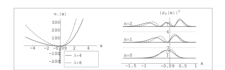
Figure 3: Non-singular and singular (attractive) potential (47) along with probability-density functions (in a.u.) associated with ground and first two excited states corresponding to $\lambda=4$ and $\lambda=6$ for $l_{1}=5,K_{3}=4,\alpha=2,\beta=\gamma=1$.

5.3 Algebraic mass and potential

As our second example, let us take the following mass function studied in Ref. [6]

$$m(x)=\left(\frac{\alpha+x^{2}}{1+x^{2}}\right)^{2}\,,\quad\alpha>0\,,\ \neq 1.$$ (48)

This mass function remains strictly positive definite everywhere and approach a constant value 1 at both infinity. The SI potential is

$$v_{+}(x;\lambda)=\frac{g^{2}}{4}-\frac{\lambda^{2}-K_{3}^{2}}{4g^{2}}-\left(\lambda+\frac{l_{1}}{2}\right)+(\alpha-1)\frac{3x^{2}-1}{(\alpha+x^{2})^{3}}-5(\alpha-1)^{2}\frac{x^{2}}{(\alpha+x^{2})^{4}}\,,$$ (49)

where

$$g(x;\lambda)=\gamma+\lambda[x+(\alpha-1)\textrm{tan}^{-1}x]\,.$$ (50)

Figure 4: Non-singular potential (49) and mass function (48), depicted in a.u., for $l_{1}=5,\gamma=1,\lambda=K_{3}=4$ corresponding to (i) $\alpha=0.3,0.6$ (first row) and (ii) $\alpha=1,10$ (second row).

The non-singular potential is given by (49) for $\lambda=K_{3}$. For $0<\alpha<1$, it is a bistable potential and for $\alpha>1$ it is a single potential well, while $\alpha=1$ recovers the constant-mass system giving harmonic oscillator well. Fig. 4 describes non-singular potential (49) and mass function (48) corresponding to (i) $\alpha=0.3,0.6$ (first row) and (ii) $\alpha=1,10$ (second row). From this Fig. it is clear that for small values of $\alpha$, the height of separator between two wells grows producing a thin barrier. On the other hand for very large values of $\alpha$, the single well becomes sharper compare to that of standard harmonic oscillator well.

The potential acquires an inverse-square singularity for $\lambda\neq K_{3}$, which is repulsive (attractive) for $0<\lambda<K_{3}$ ($\lambda>K_{3}$). For weakly repulsive singularity ($0<C<3/4$) the regular (non-singular) wave functions are given by the sequence $\{\left(\mathcal{A}^{\dagger}\right)^{n}\psi_{0,1}^{+}(x)\}$. According to the boundary conditions required to have self-adjoint extensions of the Hamiltonian, these wave functions tend to vanish at $x\rightarrow x_{0}$, $x_{0}$ being node of the function $g(x)$ given by (50). This behaviour is depicted in Fig. 5, wherein we have plotted singular potential along with probability density functions associated with first three excited levels of the sequence $\{\psi_{n}(x;\lambda)\}$ given by (42) for $\lambda=2$, other parameters being taken as $l_{1}=5,K_{3}=4,\alpha=2,\gamma=1$. These choice of parameters yields the strength $C$ and center $x_{0}$ of the singularity as $C=0.25,x_{0}=-0.26$.

Figure 5: Singular (repulsive) potential (49) and the probability-density functions (in a.u.) corresponding to non-singular wave functions associated with first three excited levels for $l_{1}=5,\alpha=2,\gamma=1,\lambda=2,K_{3}=4$.

Physically the well confining the particle is divided into two zones by a high thin barrier at $x_{0}=-0.26$. But note that for weakly repulsive case this barrier is penetrable by a quantum-mechanical particle.

5.4 SI condition in reduced first order SUSY

In subsection 5.1 we have proposed a second order SI condition (34) and consequently have obtained a new system of ES Hamiltonians $h_{+}(x;\lambda)$ where the potential $v_{+}(x;\lambda)$ and the mass $m(x)$ are related according to (36). Here we wish to show that the same system (36) (up to a constant shift) could be studied through first order SI formalism provided the Hamiltonians are factorizable according to (29) or (31). To see this, consider the 1-SUSY pair $(v_{+}\equiv v_{+}^{(2)},v_{-}^{(2)})$ given by (20) and (32) corresponding to Type II reduction (31). Here the SI parameter will be $K_{3}$ instead of $\lambda$, while the other parameters have to be considered fixed. For convenience, in the following we will use the symbol $a_{0}$ for $K_{3}$. The relation between first order superpotential $\mbox{W}_{2}(x;a_{0})$ and the mass function $m(x)$ reads from (31) and (35)

$$\mbox{W}_{2}(x;a_{0})=\frac{g(x)}{2}-\frac{m^{\prime}(x)}{4m^{3/2}(x)}+\frac{a_{0}-\lambda}{2g(x)}\,.$$ (51)

To have zero energy ground state, consider the Hamiltonian $\tilde{h}_{+}^{(2)}(x;a_{0})=h_{+}^{(2)}(x;a_{0})-K_{2}(a_{0})=\mbox{A}_{2}^{\dagger}(x;a_{0})\mbox{A}_{2}(x;a_{0})$, where the operator $\mbox{A}_{2}$ is given by (28) and $K_{2}(a_{0})=-(a_{0}+l_{1})/2$ for Type II reduction. Let us use the following abbreviations for the shifted potentials

$$\tilde{v}_{+}^{(2)}(x;a_{0})=v_{+}^{(2)}(x;a_{0})-K_{2}(a_{0})\,,\qquad\tilde{v}_{-}^{(2)}(x;a_{0})=v_{-}^{(2)}(x;a_{0})-K_{2}(a_{0})\,,$$

where $\phi_{n}^{+(2)}(x;a_{0}),\epsilon_{n}^{+(2)}$ correspond wave functions and eigenvalues. Note that the wave functions and energy eigenvalues of $h_{+}(x;\lambda)$, given by (18) and (36) are related with $\{\phi_{n}^{+(2)}(x;a_{0}),\epsilon_{n}^{+(2)}\}$ by

$$\psi_{n}^{+}(x;\lambda)\propto\phi_{n}^{+(2)}(x;a_{0})\,,\qquad E_{n}^{+}=\epsilon_{n}^{+(2)}+K_{2}\,,\quad n=0,1,\ldots$$

where $a_{0}\equiv K_{3}$. One then find from (51) following SI condition in the reduced first order SUSY

$$\tilde{v}_{-}^{(2)}(x;a_{0})=\tilde{v}_{+}^{(2)}(x;a_{1})+R(a_{1})\,,\qquad a_{1}=f(a_{0})=2\lambda-a_{0}\,,\>R(a_{1})=2\lambda-a_{1}\,.$$ (52)

Thus full spectra of $\tilde{h}_{+}^{(2)}(x;a_{0})$ can be recovered according to standard prescription

$$\left.\begin{array}[]{l}\epsilon_{0}^{+(2)}=0,\epsilon_{n}^{+(2)}=\sum_{k=1}^{n}R(a_{k})\,,\quad a_{k}=f(a_{k-1})\\[4.30554pt] \phi_{n}^{+(2)}(x;a_{0})\propto\mbox{A}_{2}^{\dagger}(x;a_{0})\mbox{A}_{2}^{\dagger}(x;a_{1})\cdots\mbox{A}_{2}^{\dagger}(x;a_{n-1})\phi_{0}^{+(2)}(x;a_{n})\end{array}\right\}\,,\quad n=1,2\ldots$$

where $\phi_{0}^{+(2)}(x;a_{0})$ is zero mode of the operator $\mbox{A}_{2}(x;a_{0})$, given by (33). Two points are to be noted. Firstly imposing the restriction of factorizability on the Hamiltonians one would come out with the SI condition (52) and the relation (51), which have not been reported so far in the literature for EM Hamiltonian. Secondly the proposed SSUSY scheme definitely leads to a generalized SI criteria (34), because in this case no such restrictions need to be imposed on the Hamiltonians.

Our final remark is that in the CM limit $m\rightarrow 1$ , both potentials $v_{+}(x;\lambda)$, given by (47) and (49) reduce to known SI potential $v_{+}^{\textrm{\tiny{CM}}}(x;\lambda)$ :

$$v_{+}^{\textrm{\tiny{CM}}}(x;\lambda)=\frac{(\gamma+\lambda x)^{2}}{4}-\frac{\lambda^{2}-K_{3}^{2}}{4(\gamma+\lambda x)^{2}}-\left(\lambda+\frac{l_{1}}{2}\right)\,,$$ (53)

and the wave functions and energy eigenvalues exactly coincide with those [46, 47] for (53).

6 Conclusion

In this article we have used SSUSY scheme for describing dynamics of a quantum particle with a position-dependent mass. We have derived a compact expression of 2-SUSY pairs $(v_{+},v_{-})$ in terms of second order superpotential $\mathcal{W}\,_{m}(x)$ and the mass function $m(x)$. A detailed analysis has been given about zero mode equations of second order supercharges and possible reduction of SSUSY scheme to first order SUSY. Based on the existence of intertwining relation between 2-SUSY partner Hamiltonians $h_{\pm}$, we have obtained a new relation between potential $v_{+}(x)$ and mass $m(x)$ leading to a simple SI condition. As a result full spectra is achieved by successive application of second order raising operator $\mathcal{A}^{\dagger}$ upon the zero modes of the lowering operator $\mathcal{A}$. It is shown that in the reduced first order SUSY approach, one may obtain a new relation between first order superpotential $\mbox{W}_{2}(x)$ and mass $m(x)$ and the same system (up to a constant shift) could possess a first order SI property provided the Hamiltonians are factorizable. The advantage of using SSUSY scheme is that it deals with a generalized but simpler SI requirement, namely partner Hamiltonians differ by a constant $\lambda$.

We have constructed explicit examples for two types of position-dependence of mass function, one is hyperbolic and the other is algebraic. The corresponding potentials have very different aspects based on the values of the SI parameter $\lambda$. Both are non-singular for $\lambda=K_{3}$, where the constant $K_{3}$ appears in the process of relating Schrödinger Hamiltonian with super Hamiltonian. The parameters $\beta$ and $\alpha$ characterizes position-dependence of mass (45) and (48) respectively. The non-singular algebraic potential (49) shares same qualitative features as those discovered in Ref. [6]. For $\lambda\neq K_{3}$, the potentials acquire an inverse square singularity, which is attractive (repulsive) for $\lambda>K_{3}$ ($\lambda<K_{3}$). The week strength of singularity ($-1/4<C<3/4$) is particularly of physical interest. Because for weakly attractive singularity ($-1/4<C<0$) the ground state energy remains finite. On the other hand, for weakly repulsive singularity ($0<C<3/4$) the barrier is penetrable by quantum-mechanical particle. In both instances, regular (non-singular) wave functions vanish at the center of the singularity.

It is important to clarify that the novelty of our work lies in the fact that we have generalized for the first time the concept of SI to the second order SUSY approach for EM Hamiltonians. In this context one should look into the explicit classification done in Ref. [16] via $\mathcal{N}$-fold SUSY approach to EM quantum systems. The systems investigated in this article belong to a special subclass of the systems studied there, which possess second order shape-invariance. Hence one has a significant advantage of obtaining wave functions and energy eigenvalues for such Hamiltonians over the existing general method for arbitrary potential and mass functions.

We would like to mention that in many practical applications, where continuous spectra is of interest [1], SSUSY scheme used here may be utilized to relate transmission and reflection amplitudes of partner Hamiltonians. The idea of SI condition for SSUSY scheme can be straightforwardly extended to general $\mathcal{N}$-th order representation ($\mathcal{N}>2$) of ladder operators. However obtaining a physical model will be much more difficult, because one has to make an appropriate choice of the mass function as well as of the coefficient functions in the ladder operators. We hope to address some of these issues elsewhere.

References

References

- [1] Bastard G 1988 Wave Mechanics Appied to Semiconductor Heterostructures (Les Editions de Physique, Les Ulis, France)
- [2] Serra L and Lipparini E 1997 Europhys. Lett. 40 667
- [3] Barranco M, Pi M, Gatica S M, Hernandez E S and Navarro J 1997 Phys. Rev. B 56 8997
- [4] Dekar L, Chetouani L and Hammann T F 1999 Phys. Rev. A 59 107
- [5] Milanović V and Ikonié Z 1999 J. Phys. A 32 7001
- [6] Plastino A R, Rigo A, Casas M, Garcias F and Plastino A 1999 Phys. Rev. A 60 4318
- [7] Dutra A de S and Almeida C A S 2000 Phys. Lett. A 275 25
- [8] Roy B and Roy P 2002 J. Phys. A 35 3961
- [9] Gönül B, Gönül B, Tutcu D and Özer O 2002 Mod. Phys. Lett. A 17 2057
- [10] Koç R, Koca M and Körcük E 2002 J. Phys. A 35 L527
- [11] Alhaidari A D 2002 Phys. Rev. A 66 042116
- [12] Dutra A de S, Hott M and Almeida C A S 2003 Europhys. Lett. 62 8
- [13] Bagchi B, Banerjee A, Quesne C and Tkachuk V M 2005 J. Phys. A 38 2929
- [14] Quesne C 2006 Ann. Phys. 321 1221
- [15] Ganguly A, Kuru Ş, Negro J and Nieto L M 2006 Phys. Lett. A 360 228
- [16] Tanaka T 2006 J. Phys. A 39 219
- [17] Ganguly A, Ioffe M V and Nieto L M 2006 J. Phys. A 39 14659
- [18] Bachelet G B, Ceperley D M and Chiocchetti M G B 1989 Phys. Rev. Lett. 62 2088
-
[19]
Junker G 1996 Supersymmetric Methods in Quantum and
Statistical Physics (Springer: Berlin)
Bagchi B K 2000 Supersymmetry in Quantum and Classical Mechanics (Chapman & Hall/CRC: Boca Ratton, Florida)
Cooper F, Khare A and Sukhatme U P 2001 Supersymmetry in Quantum Mechanics (World Scientific: Singapore) - [20] Bagchi B and Ganguly A 1998 Int. J. Mod. Phys. A 13 3711
- [21] Andrianov A A, Ioffe M V and Spiridinov V P 1993 Phys. Lett. A 174 273
- [22] Andrianov A A, Ioffe M V, Cannata F and Dedonder J P 1995 Int. J. Mod. Phys. A 10 2683
- [23] Samsonov B F 1996 Mod. Phys. Lett. A 11 1563
- [24] Fernández C D J 1997 Int. J. Mod. Phys. A 12 171
- [25] Bagchi B, Ganguly A, Bhaumik D and Mita A 1999 Mod. Phys. Lett A 14 27
- [26] Andrianov A A, Cannata F, Ioffe M V and Nishnianidze D 2000 Phys. Lett. A 266 341
- [27] Plyushchay M 2000 Int. J. Mod. Phys. A 15 3679
- [28] Aoyama H, Sato M and Tanaka T 2001 Phys. Lett. B 503 423, Nucl. Phys. B 619 105
- [29] Andrianov A A and Sokolov A V 2003 Nucl. Phys. B 660 25
- [30] González-López A and Tanaka T 2005 J. Phys. A 38 5133, 2006 ibid 39 3715
- [31] Samsonov B F 2006 Phys. Lett. A 358 105
- [32] Gendenshtein L E 1983 JETP Lett. 38 356
- [33] Frank W M, Land D J and Spector R M 1971 Rev. Mod. Phys. 43 36, pp. 92–95
- [34] Dunne G and Feinberg J 1998 Phys. Rev. D 57 1271
- [35] Ganguly A 2000 Mod. Phys. Lett. A 15 1923
- [36] Ganguly A 2002 J. Math. Phys. 43 1980, ibid 43 5310
- [37] Fernández C D J and Ganguly A 2005 Phys. Lett. A 338 203, 2007 Ann. Phys. 322 1143
- [38] BenDaniel D J and Duke C B 1966 Phys. Rev. 152 683
- [39] von Roos O 1983 Phys. Rev. B 27 7547
- [40] Morrow R A and Brownstein K R 1984 Phys. Rev. B 30 678
- [41] Einevoll G T and Hemmer P C 1988 J. Phys. C: Solid State 21 L1193
- [42] Lévy-Leblond J-M 1992 Eur. J. Phys. 13 215, 1995 Phys. Rev. A 52 1845
- [43] Yung K C and Yee J H 1994 Phys. Rev. A 50 104
- [44] Sukumar C V 1986 J. Phys. A: Math. Gen. 19 2229
- [45] Ganguly A in preparation
- [46] Lévai G 1989 J. Phys. A 22 689
- [47] Bagchi B and Ganguly A 2003 J. Phys. A 36 L161