Baryon resonances and polarization transfer in hyperon photoproduction

Abstract

A partial wave analysis of data on photoproduction of hyperons including single and double polarization observables is presented. The large spin transfer probability reported by the CLAS collaboration can be successfully described within an isobar partial wave analysis.

1 Introduction

The new CLAS data on hyperon photoproduction Bradford:2006ba show a remarkably large spin transfer probability. In the reactions $\gamma p\to\Lambda K^{+}$ and $\gamma p\to\Sigma K^{+}$ using a circularly polarized photon beam, the polarizations of the $\Lambda$ and $\Sigma$ hyperons were monitored by measurements of their decay angular distributions. For photons with helicity $h_{\gamma}=1$, the magnitude of the $\Lambda$ polarization vector was found to be close to unity, $1.01\pm 0.02$ when integrated over all production angles and all center-of-mass energies $W$. For $\Sigma$ photoproduction, the polarization was determined to be $0.82\pm 0.03$ (again integrated over all energies and angles), still a remarkably large value. The polarization was determined from the expression $\sqrt{C_{x}^{2}+C_{z}^{2}+P^{2}}$, where $C_{z}$ is the projection of the hyperon spin onto the photon beam axis, $P$ the spin projection on the normal-to-the-reaction plane, and $C_{x}$ the spin projection in the center-of-mass frame onto the third axis. The measurement of polarization effects for both $\Lambda$ and $\Sigma$ hyperons is particularly useful. The $ud$ pair in the $\Lambda$ is antisymmetric in both spin and flavour; the $ud$ quark carries no spin, and the $\Lambda$ polarization vector is given by the direction of the spin of the strange quark. In the $\Sigma$ hyperon, the $ud$ quark is in a spin-1 state and points into the direction of the $\Sigma$ spin while the spin of the strange quark is opposite to it.

Schumacher Schumacher:2006 interpreted the $\gamma p\to\Lambda K^{+}$ process on the quark level. He assumed that the circularly polarized photon with $h_{\gamma}=1$ converts into a $\phi$-meson due to vector-meson dominance; the $s\bar{s}$ pair would have helicity 1 and the spins of the $s$-quarks would then be transferred to the hyperon spin. Since the $s\bar{s}$ pair is created in the initial state, $s$-channel $N^{*}$ baryons cannot play a large role in the reaction, and the data should be explained with dominantly non-resonant contributions to the reaction amplitude. However, it is well known that resonances do play a significant role, especially in the $K^{+}\rm\Lambda$ channel. Furthermore, if the strange-quark helicity were responsible for the $\Lambda$ polarization, we should expect opposite polarizations for $\Lambda$ and $\Sigma$. This is however forbidden by selection rules: for forward and backward angles, $C_{x}$ is constrained to zero and $C_{z}$ to unity ($+1$). The model Schumacher:2006 fails to reproduce the qualitative features of $\gamma p\to\Sigma K^{+}$.

Kochelev Kochelev:2006fn argues that instantons provide a natural explanation of the strong polarization transfer. Instanton induced interactions transform initial-state quarks with left-handed (right-handed) chiralities into final-state quarks having opposite chiralities. For massless quarks, chirality coincides with helicity, so the helicities of the initial and final state should be fully correlated. It is again difficult to understand why the $\Lambda$ and the $\Sigma$ spin are both aligned with the photon polarization

The recoil (or induced) polarization $P$ can be oriented parallel or anti-parallel to the scattering-plane normal. Thus, the recoil polarizations $P_{\Lambda}$ and $P_{\Sigma}$ can have opposite signs. An opposite sign for $\Lambda$ and $\Sigma$ polarizations has been observed in a number of reactions; induced polarization is well established and not restricted to photoproduction reactions Wilkinson:1981jy . When the $\Lambda$ and $\Sigma$ polarizations in a given process point into the opposite directions and have the same magnitude, this may serve as evidence that the hadronic polarization originates from the underlying orientation of the strange quark spin. DeGrand and Miettinen DeGrand:1981pe have argued that in the presence of a strong gradient of the interaction potential, there is an effective $L\cdot S$ interaction which increases (or decreases) the scattering angle for $L\cdot S>0$ (or $L\cdot S<0$) and, thus, an effective

Figure 1: The recoil polarizations $P_{\Lambda}$ for $\gamma p\rightarrow K^{+}\rm\Lambda$ (black circles), and $P_{\Sigma}$ for $\gamma p\rightarrow K^{+}\rm\Sigma^{0}$ (open circles) Bradford:2005pt . The latter is plotted with a negative sign.

polarization asymmetry is induced. The $L\cdot S$ interaction can be experienced by the $s$ quark at the moment of $s\bar{s}$ pair creation, or at the hadron level.

Fig. 1 shows the CLAS data Bradford:2005pt on the induced polarization $P_{\Lambda}$ and, overlaid, $-P_{\Sigma}$. The induced polarizations $P_{\Lambda}$ and $P_{\Sigma}$ evidently have opposite signs and have similar magnitudes.

Independently of the question if the polarization phenomena require an interpretation on the quark or on the hadron level, the large polarization seems to contradict an isobar picture of the process in which intermediate $N^{*}$’s and $\Delta^{*}$’s play a dominant role. It is therefore important to see if the data are compatible with such an isobar interpretation or not.

2 Double polarization observables in hyperon photoproduction

Let us briefly summarize the definition and properties of the beam-recoil observables $C_{x}$ and $C_{z}$. The coordinate system $(x,y,z)$ is defined by the normal to the reaction plane $y$ and the direction of the incoming photon $z$. Following the notation given in Fasano:1992es , the polarization cross section can be written as

$$\sigma^{(B,T,R)}\equiv\frac{d\sigma^{(B,T,R)}}{d\Omega}$$ (1)

where the subscript $(B,T,R)$ denotes the polarization states of the beam, target and recoil baryon, respectively. To express the beam-recoil observables $C_{i}$, we use a rotated coordinate system with $y^{\prime}=y$ and $z^{\prime}$ defined by the direction of the outgoing kaon. The photon beam with helicity $h_{\gamma}=+1$ is marked by the subscript $r$. The beam-recoil observables $C_{x^{\prime}}$ and $C_{z^{\prime}}$ are then defined as

$$C_{x^{\prime}}=\frac{\sigma^{(r,0,+x^{\prime})}-\sigma^{(r,0,-x^{\prime})}}{\sigma^{(r,0,+x^{\prime})}+\sigma^{(r,0,-x^{\prime})}}$$

$$C_{z^{\prime}}=\frac{\sigma^{(r,0,+z^{\prime})}-\sigma^{(r,0,-z^{\prime})}}{\sigma^{(r,0,+z^{\prime})}+\sigma^{(r,0,-z^{\prime})}}$$ (2)

The properties of $C_{x^{\prime}}$ and $C_{z^{\prime}}$ are well known, its expressions in terms of CGLN (Chew-Goldberger-Low-Nambu) Chew:1957tf , helicity and multipole amplitudes can be found for example in Fasano:1992es . The CLAS collaboration measured this beam-recoil observables in the system where the z axis of the reaction plane is along the direction of the photon beam. Since the polarization is transformed like a three-vector, the transition from $C_{x^{\prime}}$,$C_{z^{\prime}}$ to $C_{x}$,$C_{z}$ follows the standard rotation matrix,

$$C_{x} = C_{x^{\prime}}\cos\theta+C_{z^{\prime}}\sin\theta$$

$$C_{z} =- C_{x^{\prime}}\sin\theta+C_{z^{\prime}}\cos\theta$$ (3)

where $\theta$ is the scattering angle of the kaon. The $C_{x^{\prime}}$,$C_{z^{\prime}}$ or $C_{x}$,$C_{z}$ observables have defined values at forward and backward scattering angles. Helicity conservation requires $C_{x}=0$ and $C_{z}=1$ at $\theta=0,180$. This feature is model independent and, of course, compatible with the CGLN amplitudes. Hence, $C_{z}=1$ holds for both, for the photoproduction of $K^{+}\rm\Lambda$ and of $K^{+}\rm\Sigma^{0}$.

The double polarization observables $C_{x}$ and $C_{z}$ have an important constraint given by Barker:1975bp

$$C_{x}^{2}+C_{z}^{2}\leq\;Min((1-\Sigma^{2}),(1-P^{2}))$$ (4)

where $\Sigma$ is the beam asymmetry and $P$ the recoil polarization. Evidently, there is a strong connection between $C_{i}$ and single polarization observables.

3 The partial wave formalism

The partial wave analysis presented here is based on relativistically invariant amplitudes constructed from the four-momenta of particles involved in the process Anisovich:2004zz . High-spin resonances are described by relativistic multi-channel Breit-Wigner amplitudes, important partial waves with low total spin ($J<5/2$) are described in the framework of the K-matrix/P-vector approach which automatically satisfies the unitarity condition. The amplitude for elastic scattering is given by

$$\hat{A}(s)\;=\;\hat{K}\;(\hat{I}\;-\;i\hat{\rho}\hat{K})^{-1}\,.$$ (5)

The phase space matrix $\hat{\rho}$ is a diagonal matrix. The two particle phase space was used in the form calculated in Anisovich:2006bc :

$$\rho(s)=\frac{\alpha_{L}}{2L+1}\frac{2|\vec{k}|^{2L+1}}{\sqrt{s}}\frac{k_{10}+m_{N}}{2m_{N}}\frac{F(\vec{k}^{2})}{B(L,r,\vec{k}^{2})}$$ (6)

where $s$ is the total energy squared, $k$ is the relative momentum between baryon and meson, $k_{10}$ is the energy of the baryon (with mass $m_{N}$) calculated in the c.m.s. of the reaction and the coefficient $\alpha_{L}$ is equal to:

$$\alpha_{L}=\prod\limits_{n=1}^{L}\frac{2n-1}{n}\,.$$ (7)

For regularization of the phase volume at large energies we used a standard Blatt-Weisskopf form factor with $r=0.8$ fm and a form factor $F(k^{2})$ using two different forms:

$$F(k^{2})=\frac{\Lambda+0.5}{\Lambda+\vec{k}^{2}}\,,\qquad F(k^{2})=\frac{\Lambda+2.5}{\Lambda+s}\,,$$ (8)

Fits with both parameterizations produced a very similar result. The parameter $\Lambda$ was fixed from our previous analysis Anisovich:2005tf ; Sarantsev:2005tg and was not varied in the present fit. For the first parameterization it was taken to be equal to 1.5 and for the second one 3.0. Below threshold the two body phase volumes were continued with the subtracted dispersion integral:

$$i\rho(s)\;\to\int\limits_{(m_{N}\!+\!m_{\mu})^{2}}^{\infty}\!\!\!\!\frac{\rho(s^{\prime})(s-(m_{N}\!+\!m_{\mu})^{2})}{(s^{\prime}-s)(s^{\prime}-(m_{N}\!+\!m_{\mu})^{2})}\frac{ds^{\prime}}{\pi}\ ,$$ (9)

where $m_{\mu}$ is the meson mass in the decay channel. The exact formulas for the three body phase volumes are given in Anisovich:2006bc .

The photoproduction amplitude can be written in the P-vector approach. The P-vector amplitude is then given by

$$A_{a}\;=\;\hat{P}_{b}\;(\hat{I}\;-\;i\hat{\rho}\hat{K})^{-1}_{ba}\,.$$ (10)

The production vector $\hat{P}$ and the K-matrix $\hat{K}$ have the following parameterizations:

$$K_{ab}\;=\;\sum_{\alpha}\frac{g_{a}^{(\alpha)}g_{b}^{(\alpha)}}{M^{2}_{\alpha}-s}\;+\;f_{ab},\;\;\;P_{b}\;=\;\sum_{\alpha}\frac{g_{\gamma\rm N}^{(\alpha)}g_{b}^{(\alpha)}}{M^{2}_{\alpha}-s}\;+\;\tilde{f}_{b}$$

(11)

where $M_{\alpha}$, $g_{a}^{(\alpha)}$ and $g_{\gamma\rm N}^{(\alpha)}$ are the mass, coupling constant and photo-coupling of the resonance $\alpha$; $f_{ab}$ describes direct non-resonant transition processes from an initial state $a$ to a final state $b$, e.g. from $N\pi\to\Lambda K$ The production process may have a non-resonant contribution due to $\tilde{f}_{b}$. In general, these non-resonant contributions are functions of $s$.

For all partial waves except $S_{11}$, it is sufficient to assume $f_{ab}$ and $\tilde{f}_{b}$ to be constants. Only the $S_{11}$ wave requires a slightly more complicated structure. For the scattering amplitudes $\pi N\to N\pi$, $\pi N\to N\eta$, and $\eta N\to N\eta$ we choose

$$f_{ab}=\frac{f_{ab}^{(1)}+f_{ab}^{(2)}\sqrt{s}}{s-s_{0}^{ab}}\,.$$ (12)

This form is similar to the one used by SAID Arndt:2006bf . The $f_{ab}^{(i)}$ and $s_{0}^{ab}$ are constants which are determined in the fits.

The P-vector approach is based on the idea that a channel with a weak coupling can be omitted from the K-matrix. Indeed, adding to the K-matrix the $\gamma N$ channel would not change the properties of the amplitude. Due to its weak coupling, the $\gamma N$ interaction can be taken into account only once; this is done in the form of a P-vector. Loops due to virtual decays of a resonance into $N\gamma$ and back into the resonance can be neglected safely. A similar approach can be used to describe also decay modes with a weak coupling. The amplitude for the transition into such a channel can be written as D-vector amplitude,

$$A_{a}\;=\;\hat{D}_{a}+[\hat{K}(\hat{I}\;-\;i\hat{\rho}\hat{K})^{-1}\,\hat{\rho}]_{ab}\hat{D}_{b}\;,$$ (13)

Table 1: Properties of the $P_{11}$ $K$-matrix poles for one of the solutions. The masses, widths, and $g$ are given in GeV, the helicities $A$ in GeV${}^{-\frac{1}{2}}$, $s$ in GeV²; the $f$ are dimensionless.

		Pole 1	Pole 2	Pole 3
	$M$	1516$\pm$30	1722$\pm$35	2233$\pm$50
	$A_{1/2}$	-0.031	0.022	-0.067
$a$		$g^{(1)}_{a}$	$g^{(2)}_{a}$	$g^{(3)}_{a}$	$f_{1a}$
1	$N(940)\pi$	1.052	-0.156	1.226	-1.736
2	$\Lambda K^{+}$	0	-0.003	-0.556	0
3	$\Sigma K^{+}$	0	0.709	0.063	0

Table 2: Properties of the $P_{13}$ $K$-matrix poles for one of the solutions.

		Pole 1	Pole 2	Pole 3
	$M$	1770$\pm$50	1880$\pm$50	2195$\pm$50
	$A_{1/2}$	0.022	0.010	0.202
	$A_{3/2}$	0.051	0.039	-0.069
$a$		$g^{(1)}_{a}$	$g^{(2)}_{a}$	$g^{(3)}_{a}$	$f_{1a}$
1	$N(940)\pi$	0.650	0.206	-1.200	-1.237
2	$N(940)\eta$	0.900	0.811	-0.440	-0.962
3	$\Lambda K^{+}$	0.900	0.560	-0.849	-0.016
4	$\Sigma K^{+}$	-0.319	0.727	-0.202	1.050

Table 3: Properties of the $S_{11}$ $K$-matrix poles for one of the solutions.

		Pole 1	Pole 2
	$M$	1420$\pm$80	1710$\pm$30
	$A_{1/2}$	0.125	0.093
$a$		$g^{(1)}_{a}$	$g^{(2)}_{a}$	$f_{1a}^{(1)}$	$f_{2a}^{(1)}$
1	$N(940)\pi$	0.074	0.844	1.651	-1.970
2	$N(940)\eta$	-1.908	-0.434	-1.970	2.010
3	$\Lambda K^{+}$	-0.300	-0.346	-0.016	-0.432
4	$\Sigma K^{+}$	-1.232	-0.804	-0.497	3.663
		$f_{1\alpha}^{(2)}$	$s_{0}^{1a}$	$f_{2a}^{(2)}$	$s_{0}^{2a}$
1	$N(940)\pi$	-1.285	0.430	0.625	-0.620
2	$N(940)\eta$	0.625	-0.620	1.990	0.600

where the parameterization of the D-vector is similar to the parameterization of the P-vector in (11). As in the case of the P-vector approach, channels with weak couplings can be taken into account only in their real decay, not as virtual loops.

In case where both initial and final coupling constants are weak, we used the so-called PD-vector approximation. In this case the amplitude is given by

$$A_{ab}\;=\;\hat{G}_{ab}+\hat{P}_{a}(\hat{I}\;-\;i\hat{\rho}\hat{K})^{-1}\,\hat{\rho}\hat{D}_{b}\;,$$ (14)

where $\hat{G}$ corresponds to direct production from state ${}^{\prime}a^{\prime}$ decaying into state ${}^{\prime}b^{\prime}$. The P-vector and D-vectors are defined above.

To facilitate the interpretation of the formalism we give in Tables 3–3 the full parametrization of the K-matrices for the $P_{11}$, $P_{13}$, and $S_{11}$ waves for one of the two solutions discussed below.

4 Data and fits

The data used in this analysis comprise differential cross section for $\gamma p\to K^{+}\rm\Lambda$, $\gamma p\to K^{+}\rm\Sigma^{0}$, and $\gamma p\to\Sigma^{+}K^{0}_{s}$ including their recoil polarization and the photon beam asymmetry, and the recent spin transfer measurements Bradford:2006ba ; Bradford:2005pt ; Glander:2003jw ; McNabb:2003nf ; Lleres:2007tx ; Zegers:2003ux ; Lawall:2005np ; Castelijns:2007qt . Furthermore, data are included from the SAID data base Bartholomy:04 ; Bartalini:2005wx ; SAID1 ; SAID ; SAID2 ; Crede:04 ; Krusche:nv ; GRAAL2 ; Bartalini:2007fg on photoproduction of $\pi^{0}$ and $\eta$ with measurements of differential cross sections, beam and target asymmetries and recoil polarization. We did not use the $K^{+}\rm\Sigma^{0}$ recoil polarization data from Lleres:2007tx since they have larger errors and a smaller energy range than the CLAS data.

The fit also used data on photo-induced $2\pi^{0}$ production Thoma:2007 ; Sarantsev:2007 and $\pi^{0}\eta$ Horn:2007 and the recent BNL data on $\pi^{-}p\to n\pi^{0}\pi^{0}$ Prakhov:2004zv in an event-based likelihood fit. $2\cdot\ln\mathcal{L}$ was added to the pseudo-$\chi^{2}$ function. The data essentially determined the contributions of isobars to the $N\pi\pi$ and $N\pi\eta$ final state and are not discussed here further. Details can be found in Thoma:2007 ; Sarantsev:2007 ; Horn:2007 .

Table 4: Single meson photoproduction data used in the partial wave analysis and $\chi^{2}$ for solutions 1 and 2.

Observable	$N_{\rm data}$	$w_{i}$	$\frac{\chi^{2}}{N_{\rm data}}$	$\frac{\chi^{2}}{N_{\rm data}}$	Ref.
			Sol. 1	Sol. 2
$C_{x}(\rm\gamma p\rightarrow\Lambda K^{+})$	160	5	1.71	1.66	Bradford:2006ba
$C_{z}(\rm\gamma p\rightarrow\Lambda K^{+})$	160	7	1.95	2.34	Bradford:2006ba
$\rm\sigma(\gamma p\rightarrow\Lambda K^{+})$	1377	5	2.02	1.99	Bradford:2005pt
$\rm\sigma(\gamma p\rightarrow\Lambda K^{+})$	720	1	1.53	1.55	Glander:2003jw
$\rm P(\gamma p\rightarrow\Lambda K^{+})$	202	6.5	1.65	2.28	McNabb:2003nf
$\rm P(\gamma p\rightarrow\Lambda K^{+})$	66	3	2.89	1.05	Lleres:2007tx
$\Sigma(\rm\gamma p\rightarrow\Lambda K^{+})$	66	5	2.19	2.85	Lleres:2007tx
$\Sigma(\rm\gamma p\rightarrow\Lambda K^{+})$	45	10	1.98	1.82	Zegers:2003ux
$C_{x}(\rm\gamma p\rightarrow\Sigma^{0}K^{+})$	94	5	2.70	3.50	Bradford:2006ba
$C_{z}(\rm\gamma p\rightarrow\Sigma^{0}K^{+})$	94	5	2.77	2.24	Bradford:2006ba
$\rm\sigma(\gamma p\rightarrow\Sigma^{0}K^{+})$	1280	3	2.10	2.19	Bradford:2005pt
$\rm\sigma(\gamma p\rightarrow\Sigma^{0}K^{+})$	660	1	1.33	1.41	Glander:2003jw
$\rm P(\gamma p\rightarrow\Sigma^{0}K^{+})$	95	6	1.58	1.94	McNabb:2003nf
$\Sigma(\rm\gamma p\rightarrow\Sigma^{0}K^{+})$	42	5	1.04	1.34	Lleres:2007tx
$\Sigma(\rm\gamma p\rightarrow\Sigma^{0}K^{+})$	45	10	0.62	0.76	Zegers:2003ux
$\rm\sigma(\gamma p\rightarrow\Sigma^{+}K^{0})$	48	2.3	3.51	3.41	McNabb:2003nf
$\rm\sigma(\gamma p\rightarrow\Sigma^{+}K^{0})$	120	5	0.98	1.09	Lawall:2005np
$\rm\sigma(\gamma p\rightarrow\Sigma^{+}K^{0})$	72	5	1.17	0.77	Castelijns:2007qt
$\rm\sigma(\gamma p\rightarrow p\pi^{0})$	1106	7	0.99	1.03	Bartholomy:04
$\rm\sigma(\gamma p\rightarrow p\pi^{0})$	861	3	3.22	2.44	Bartalini:2005wx
$\Sigma(\rm\gamma p\rightarrow p\pi^{0})$	469	2.3	3.75	3.35	Bartalini:2005wx
$\Sigma(\rm\gamma p\rightarrow p\pi^{0})$	593	2.3	2.13	2.20	SAID1
$\rm P(\rm\gamma p\rightarrow p\pi^{0})$	594	3	2.58	2.54	SAID
$\rm T(\rm\gamma p\rightarrow p\pi^{0})$	380	3	3.85	3.90	SAID
$\rm\sigma(\gamma p\rightarrow n\pi^{+})$	1583	2.8	1.07	1.27	SAID2
$\rm\sigma(\gamma p\rightarrow p\eta)$	667	30	0.84	0.77	Crede:04
$\rm\sigma(\gamma p\rightarrow p\eta)$	100	7	1.69	1.97	Krusche:nv
$\Sigma(\rm\gamma p\rightarrow p\eta)$	51	10	1.82	1.91	GRAAL2
$\Sigma(\rm\gamma p\rightarrow p\eta)$	100	10	2.11	2.24	Bartalini:2007fg
$\gamma\to p2\pi^{0}$	160k	3	likelihood fit		Thoma:2007
$\gamma\to p\pi^{0}\eta$	16k	5	likelihood fit		Horn:2007
$\pi^{-}p\to n2\pi^{0}$	180k	2.5-4	likelihood fit		Prakhov:2004zv
$P_{11}(\pi N\to N\pi)$	110	20	1.60	1.74	Arndt:2006bf
$P_{13}(\pi N\to N\pi)$	134	10	3.78	2.83	Arndt:2006bf
$S_{11}(\pi N\to N\pi)$	126	30	1.86	1.84	Arndt:2006bf
$D_{33}(\pi N\to N\pi)$	108	12	1.88	2.69	Arndt:2006bf

Data on $\pi N$ elastic data from the SAID data base Arndt:2006bf were used for those partial waves which are described by a K-matrix.

Fits were performed using a pseudo-$\chi^{2}$ function

$$\chi^{2}_{\rm tot}=\chi^{2}_{\rm 2b}\;-\;2\ln\mathcal{L}\ ,\quad\chi^{2}_{\rm 2b}=\frac{\sum w_{i}\chi^{2}_{i}}{\sum w_{i}\,N_{i}}\,\sum N_{i}\ ,$$ (15)

where the $N_{i}$ are given as $N_{\rm data}$ (per channel) in the second and the weights in the third column of Table 4. The data were fitted with weights $w_{i}$ which ensure that low-statistics data are described reasonably well. Without weights, high-statistics data enforce a very good description, without taking into account any model imperfections, while low-statistics data would be reproduced badly in fits.

Table 5 summarizes the resonances used in our fits. In addition, amplitudes for some further resonances are included which make minor contributions to photoproduction, $N(1700)D_{13}$, $N(1710)P_{11}$, $N(1875)D_{13}$, $N(2000)F_{15}$, $N(2170)D_{13}$, $N(2200)P_{13}$,  $\Delta(1600)P_{33}$,  $\Delta(1905)F_{35}$,
$\Delta(1920)P_{33}$, $\Delta(1950)F_{37}$, and amplitudes representing $t$- and $u$-channel exchanges. The $S_{11}$-wave was fitted as 2-pole 5-channel K-matrix ($\pi N$, $\eta N$, $K\Lambda$, $K\Sigma$, $\Delta(1232)\pi$); the $P_{11}$-wave as 3-pole 4-channel K-matrix ($\pi N$, $\Delta(1232)\pi$, $K\Sigma$ and $N\sigma$) and $D_{33}$-wave as 2-pole 3-channel K-matrix ($\pi N$, $\Delta(1232)\pi$ ($S$ and $D$-waves)). The $P_{13}$ K-matrix was approximated as 3-pole 8-channel K-matrix with $\pi N$, $\eta N$, $\Delta(1232)\pi$ (P- and F-waves), $N\sigma$, $D_{13}(1520)\pi$, $K\Lambda$ and $K\Sigma$ channels.

Table 5: Baryon resonances used in the fits. All resonances listed contribute more than 4% of the intensity to at least one of the photo-production reactions listed in Table 4. The underlined resonances provide a significant fraction to hyperon photoproduction. Further resonances are needed to achieve a good fit.

$N(1440)P_{11}$	$N(1520)D_{13}$	$N(1535)S_{11}$	$N(1650)S_{11}$
$N(1675)D_{15}$	$N(1680)F_{15}$	$N(1720)P_{13}$	$N(1840)P_{11}$
$N(1900)P_{13}$	$N(2070)D_{15}$		$\Delta(1232)P_{33}$
$\Delta(1620)S_{31}$	$\Delta(1700)D_{33}$	$\Delta(1940)D_{33}$	$\Delta(1950)F_{37}$

A $\chi^{2}_{\rm 2b}$ of better than 20.000 was reached for 16.000 data points. In spite of the use of differential cross sections, of single and double polarization observables, the results of the fits depended on the starting values. Two separate classes of solutions were found, giving rather different isobar contributions. These will be compared in the discussion of the data. The two classes of solutions will be called solution 1 and 2, respectively.

One new resonance is added to describe the new CLAS data, the $N(1900)P_{13}$, for which so far, evidence had been weak only. It is surprising that the new very significant data on $C_{x}$ and $C_{z}$ are well described by introducing just one single resonance to the model. Compared to our previous analysis Anisovich:2005tf ; Sarantsev:2005tg , the $\Delta(1600)P_{33}$ and $N(1710)P_{11}$ have been introduced when the data on two-pion production and the elastic $\pi N$ scattering amplitude were included in the fit Thoma:2007 ; Sarantsev:2007 . Here, just $N(1900)P_{13}$ was added. We also tried to introduce additional resonances, one by one, in the $1/2^{\pm}$, 3$/2^{\pm}$, $5/2^{\pm}$, $7/2^{\pm}$, $9/2^{\pm}$ partial waves, without finding a significant improvement.

    

Figure 2: The total cross section for $\gamma p\rightarrow K^{+}\rm\Lambda$ Bradford:2005pt for solution 1 (a) and solution 2 (b). The solid curves are the results of our fits, dashed lines are the $P_{13}$ contribution, dotted lines are the $S_{11}$ contribution and dash-dotted lines are the contribution from $K^{*}$ exchange.

    

Figure 3: The total cross section for $\gamma p\rightarrow K^{+}\rm\Sigma^{0}$ Bradford:2005pt for solution 1 (a) and solution 2 (b). The solid curves are the results of our fits, dashed lines are the $P_{13}$ contribution, dash-dotted lines are the $P_{31}$ contribution and dotted lines are the contribution from $K$ exchange.

Figure 4: Differential cross sections for $\gamma p\rightarrow K^{+}\rm\Lambda$ (left) and $\gamma p\to K^{+}\rm\Sigma^{0}$ (right) Bradford:2005pt . Only energy bins where $C_{x}$ and $C_{z}$ were measured are shown. The solution 1 is shown as solid line and solution 2 (hardly visible since overlapping) as a dashed line. The total energy is given in MeV.

Figure 5: The beam asymmetries as a function of $W$ for $\rm\gamma p\to K^{+}\Lambda$ (left) and $\rm\gamma p\to K^{+}\Sigma$ (right) Lleres:2007tx . The solid and dashed curves are the result of our fit obtained with solution 1 and 2, respectively.

Figure 6: Double polarization observables $C_{x}$ (black circle) and $C_{z}$ (open circle) for $\rm\gamma p\to K^{+}\rm\Lambda$ (top panel) and $\rm\gamma p\to K^{+}\rm\Sigma^{0}$ (bottom panel) Bradford:2006ba . The solid and dashed curves are results of our fit obtained with solution 1 (left) and solution 2 (right) for $C_{x}$ and $C_{z}$, respectively.

Figure 7: The recoil polarization asymmetries as a function of $W$ for $\rm\gamma p\to K^{+}\Lambda$ (left) and $\rm\gamma p\to K^{+}\Sigma^{0}$ (right) from CLAS McNabb:2003nf (open circle) and GRAAL (black circle) Lleres:2007tx . The solid and dashed curves are the result of our fit obtained with solution 1 and 2 respectively.

The $\gamma p\to K^{+}\rm\Lambda$ differential cross section was measured recently by CLAS with large statistics Bradford:2005pt . The total cross section in Fig. 3 does not show a narrow peak in the $\gamma p\rightarrow K^{+}\rm\Lambda$ cross section at 1700 MeV as suggested by older data Glander:2003jw ; McNabb:2003nf but for which we did not find a physical interpretation in our previous fits Anisovich:2005tf ; Sarantsev:2005tg . The SAPHIR data are still included using a relative normalisation function as described in Sarantsev:2005tg . The total cross section seems to be better described by solution 1. However, the quality of the description of the angular distributions is very similar for both solutions (see Fig. 5); discrepancies in the total cross sections are due to the extrapolation into regions where no data exist. Hence, the total cross section cannot be used to favor solution 1 over solution 2. Note, that the total cross section is calculated as sum of the measured differential cross sections and the integrated fit result for the angular region where data are not available.

The total and differential cross sections for $\gamma p\!\to\!K^{+}\rm\Sigma^{0}$ are presented in Fig. 3 and in the right panel of Fig. 5. The quality of the description is as good as that obtained without double polarization data taken into account.

The GRAAL collaboration Lleres:2007tx measured the $K^{+}\rm\Lambda$ and $K^{+}\rm\Sigma^{0}$ beam asymmetries in the region from threshold to $W=1906$ MeV. These data are an important addition to the LEPS data of the beam asymmetry Zegers:2003ux which cover the energy region from $W=1950$ MeV to $2300$ MeV. Data and fits are shown in Fig. 5.

Fig. 6 shows the data on $C_{x}$ and $C_{z}$ and the fit obtained with solution 1 and 2. This is the data which gave the surprising large value for the spin transfer probability from the circularly polarized photon in the initial state to the final state hyperon. For both observables a very satisfactory agreement between data and fit is achieved. Small deviations show up in two mass slices in the 2.1 GeV mass region. These should however not be over-interpreted. $C_{x}^{2}+C_{z}^{2}+P^{2}$ is constrained by unity; in the corresponding mass- and $\cos\Theta_{K}$ bins, $C_{z}^{2}$ and the recoil polarization are sizable pointing at a statistical fluctuation beyond the physical limits. Of course, a fit must not follow data into not allowed regions.

Finally, the GRAAL collaboration measured also the recoil polarization Lleres:2007tx for which data from CLAS McNabb:2003nf had been measured in the region from threshold up to 2300 MeV. These data are reproduced in Fig. 7.

The fits return parameters for each partial waves. From one of the Tables 3-3 (and similar tables for other resonances), the complex amplitude (13) can be calculated using the equations (6) and (9) to calculated the phase space integral. These complex amplitudes have poles in the complex $\sqrt{s}$ plane. Setting the real or imaginary part of the amplitude to zero defines lines in the $\sqrt{s}$ plane which cross at the positions of a pole. This procedure is done for the different Rieman sheets; the pole closest to the real axis defines mass and width of the resonance. This plane and the contour lines defining the pole positions are shown in Fig. 8 for the $P_{11}$ partial wave.

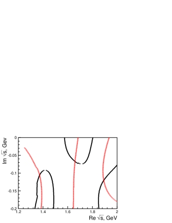
Figure 8: Contour lines defined by setting real or imaginary part of the $P_{11}$ amplitude to zero. The crossing points define the pole positions.

The coupling constants $g_{a}^{(\alpha)}$ defined in (11) give the strength of the coupling of a K-matrix pole $\alpha$ to channel $a$. We are, of course, interested in the couplings of the resonance $\alpha$ which is defined by its poles of the full amplitude or T-matrix poles. These couplings, called $\tilde{g}_{a}^{(\alpha)}$ here, are calculated as residues of the T-matrix amplitudes at the pole positions. For narrow resonances, the residues are real and can be compared to PDG values. For wide resonances, the partial widths are functions of $s$, and the residues acquire phases. To get partial decay widths which can be compared to other results, we determined the non-relativistic Breit-Wigner amplitude which reproduced the exact pole position of the full amplitude; the branching ratios given in the Table 6 were calculated at the position of the Breit-Wigner mass. When this procedure was applied to an amplitude initially parameterized as Breit-Wigner amplitude, then the original parameters were reproduced within 1-2 MeV even in the case of very large couplings and rapidly increasing phase volumes. The method works very reliably, too, for the K-matrix parameterization, even with interfering poles. However, the approach is less stable when a pole is situated close to a threshold and when the pole structure becomes complicated. In this case, we calculated the residues for both poles and increased the errors to take into account both results. In the first solution, the strong interference between the two lowest $P_{13}$ poles required such an increased systematic error.

The partial widths of a resonance are related to the coupling $g_{a}$ by

$$m_{0}\Gamma_{a}=g^{2}_{a}\rho(m_{0})$$ (16)

where $\rho(m_{0})$ is the phase space defined in (6), calculated at the real part of the pole position. To minimize the errors, we determine the decay mode fractions which do not contain the error of the total width.

5 Evidence for the $N(1900)P_{13}$

The fits described in this paper used a number of new reactions, and a variety of different results were obtained which are submitted in parallel as letter communications. These publications report results from the same fits to all reactions listed in Table 4. The reaction $\gamma p\to p\pi^{0}\pi^{0}$ was studied by the CBELSA collaboration Thoma:2007 . The analysis returned decays of baryon resonances in the third resonance region into $p\pi^{0}\pi^{0}$ via different isobars like $\Delta(1232)\pi$,
$N(\pi\pi)_{\rm S-wave}$, $N(1440)\pi$, and others. In connection with precise low-energy data on $\gamma p\to p\pi^{0}\pi^{0}$ of the A2/TAPS collaboration at MAMI, properties of the Roper resonance were derived Sarantsev:2007 . The reaction $\gamma p\to p\pi^{0}\eta$ Horn:2007 required introduction of a $\Delta(1940)D_{33}$ which is suggested to form, jointly with $\Delta(1900)S_{31}$ and $\Delta(1930)D_{35}$, a triplet of resonances at a rather low mass, incompatible with quark model calculations. The new CLAS data on $C_{x}$ and $C_{z}$ require introduction of a $N(1900)P_{13}$ resonance; without it no good description of the data was reached Nikonov:2007 . Since this paper is mainly concerned with hyperon photoproduction, we report here the main reasons why this resonance is required by the data.

The effect of removing the $N(1900)P_{13}$ resonance from the fit can be seen in figure 1 of Nikonov:2007 . The fit quality changes by $\chi^{2}_{\rm tot}=1540$ units. The $N(1900)P_{13}$ was replaced by resonances with other quantum numbers. Replacing it by an $S_{11}$ {or $D_{15}$} state, $\chi^{2}_{\rm 2b}$ changed by 950

Figure 9: Real (a) and imaginary (b) part of the $P_{13}$ elastic scattering amplitude Arndt:2006bf in comparison to the fit, solution 1 (solid curve) and solution 2 (dashed curve).

{970} only. Using $P_{11}$ quantum numbers (instead of $P_{13}$) gave $\Delta\chi^{2}_{\rm 2b}=205$ only. An $F_{15}$ state improved $\chi^{2}_{\rm 2b}$ marginally; introducing $F_{17}$ and $G_{17}$ did not improve the fit. A resonance with $P_{33}$ quantum numbers provided a change in $\chi^{2}_{\rm 2b}$ which was smaller by a factor 2 than the one found for a $P_{13}$ state.

In a final step, the $P_{13}$ was parameterized as 3-pole 8-channel K-matrix with $\pi N$, $\eta N$, $\Delta(1232)\pi$ ($P$ and $F$-waves), $N\sigma$, $D_{13}(1520)\pi$ ($S$-wave), $K\Lambda$ and $K\Sigma$ channels. This resulted in the fit solutions 1 and 2 which both are compatible with a large body of data. Both solutions are compatible with elastic $\pi N$ scattering. Real and imaginary part of the $P_{13}$ partial wave Arndt:2006bf are satisfactorily described for invariant masses up to 2.4 GeV, see Fig. 9. From the fit, properties of resonances in the $P_{13}$-wave were derived. The lowest-mass pole is identified with the established $N(1720)P_{13}$, the second pole with the badly known $N(1900)P_{13}$. A third pole is introduced at about 2200 MeV. It improves the quality of the fit in the high-mass region but its quantum numbers cannot be deduced safely from the present data base.

The parameters of the two lowest $P_{13}$ poles are collected in Table 6. The first $P_{13}$ state was found to be much broader than suggested by most other analyses Yao:2006px . However, the only analysis taking $N\pi\pi$ data into account gives a width of $(380\pm 180)$ MeV Manley:1992yb . The most recent analysis of elastic scattering data Arndt:2006bf gave a 355 MeV width. The elastic width of the $N(1720)P_{13}$ ($\approx 45$ MeV) is even narrower than the $N(1680)F_{15}$ elastic width $\approx 85$ MeV). Given the large spread of pole positions reported in Yao:2006px , we do not think that our result is in conflict with previous work.

In the first solution, the double structure in the $P_{13}$ partial wave (see Fig. 3a) is due to a strong interference between the first and the second pole. If the structure is fitted with one pole, the pole must have a rather narrow width. The $N(1720)P_{13}$ couples strongly to $\Delta(1232)\pi$ and, in the second solution, also to the $D_{13}(1520)\pi$ channel. The $D_{13}(1520)\pi$ threshold is close to its mass and creates a double pole structure which makes difficult the definition of helicity amplitudes and of decay partial widths. The method used here is described in Nikonov:2007 .

Table 6: Properties of the two lowest $P_{13}$ resonances for both solutions. The masses, widths are given in MeV, the branching ratios in % and helicity couplings in 10^-3 GeV^-1/2. The helicity couplings and phases were calculated as residues in the pole position.

	Solution 1		Solution 2
$M_{pole}$	$1640\pm 80$	$1870\pm 15$	$1630\pm 60$	$1960\pm 15$
$\Gamma_{tot}^{pole}$	$480\pm 80$	$170\pm 30$	$440\pm 60$	$195\pm 25$
$A_{1/2}$	$140\pm 80$	$-(10\pm 15)$	$160\pm 40$	$-(18\pm 8)$
$\varphi_{1/2}$	$-(10\pm 15)^{\circ}$	–	$(10\pm 15)^{\circ}$	$-(40\pm 15)^{\circ}$
$A_{3/2}$	$150\pm 80$	$-(40\pm 15)$	$70\pm 30$	$-(35\pm 12)$
$\varphi_{3/2}$	$-(40\pm 30)^{\circ}$	$(30\pm 25)^{\circ}$	$(0\pm 20)^{\circ}$	$-(40\pm 15)^{\circ}$
${\rm Br}_{N\pi}$	$8\pm 4$	$5\pm 3$	$18\pm 5$	$6\pm 3$
${\rm Br}_{N\eta}$	$14\pm 4$	$20\pm 8$	$10\pm 2$	$15\pm 3$
${\rm Br}_{K\Lambda}$	$16\pm 6$	$15\pm 5$	$7\pm 2$	$12\pm 3$
${\rm Br}_{K\Sigma}$	$<2$	$22\pm 8$	$<1$	$8\pm 2$
${\rm Br}_{\Delta\pi(P)}$	$54\pm 10$		$36\pm 6$
${\rm Br}_{\Delta\pi(F)}$	$2\pm 2$		$18\pm 5$
${\rm Br}_{D_{13}\pi}$	$2\pm 2$		$5\pm 3$
${\rm Br}_{N\sigma}$	$4\pm 2$		$4\pm 2$
${\rm Br}_{Add}$	$<2$	$38\pm 12$	$2\pm 2$	$60\pm 6$

The $N(1900)P_{13}$ is of special interest for baryon spectroscopy. It belongs to the two-star positive-parity $N^{*}$ resonances in the 1900 - 2000 MeV mass interval – $N(1900)P_{13}$, $N(2000)F_{15}$, $N(1990)F_{17}$ – which cannot be assigned to quark-diquark oscillations Santopinto:2004hw when the diquark is treated as point-like object with zero spin and isospin. At the present status of our knowledge on baryon excitations, most four-star and three-star baryon resonances can be interpreted in a simplified model describing baryons as being made up from a diquark and a quark. Evidence for the $N(1900)P_{13}$ has been communicated already in a letter publication Nikonov:2007 . The $N(2000)F_{15}$ is included in the analysis as well; it is a further two-star $N^{*}$ resonances which cannot be assigned to quark-diquark oscillations. The evidence for this state from this analysis is, however, weaker. The $N(1840)P_{11}$ state (which we now find at 1880 MeV) could be the missing partner of a super-multiplet of nucleon resonances having – as leading configuration – intrinsic orbital angular momentum $\ell=2$ and a total quark spin $s=3/2$. These angular momenta couple to a series $J=\frac{1}{2},\frac{3}{2},\frac{5}{2},\frac{7}{2}$. Yet in this analysis, there was no need to introduce $N(1990)F_{17}$.

6 Discussion

Triggered by the measurement of the spin transfer coefficients $C_{x}$ and $C_{z}$ we have refitted data on single $\pi$, $\eta$, $K^{0}$ and $K^{+}$ photoproduction. Besides $C_{x}$ and $C_{z}$ the new data on unpolarised differential cross section for $\gamma N\to K^{+}\rm\Lambda$, $\gamma N\to K^{+}\rm\Sigma^{0}$, and $K^{0}\Sigma^{+}$ photoproduction, and double pion production data were added to the combined analysis. The refit was motivated by the bad prediction of the spin transfer coefficients with our previous partial wave analysis. All data sets can be described well after introducing a $N(1900)P_{13}$ resonance. Its mass and width are estimated to $1915\pm 50$ MeV and $180\pm 50$ MeV, respectively. This result covers the two K-matrix solutions found here: in the first one, the pole position of the second $P_{13}$ state is located at $1870-i\,85$ MeV and in the second solution at $1960-i88$ MeV. The reason for the ambiguity is likely connected with the existence of a $P_{11}$ state with similar mass and width.

Even though the description of all distributions is very reasonable, the two solutions have remarkably different isobar contributions. In solution 1, the $P_{13}$ partial wave shows a significant double structure (not present in solution 2). The $S_{11}$ wave is much stronger in solution 2.

The new $P_{13}$ state Nikonov:2007 also improves the description of the $\gamma p\to K^{+}\rm\Sigma^{0}$ reaction. However the effect from introducing this state is much smaller here. Actually, in our previous analysis, the double polarization data of this channel were already described much better than those for $\gamma p\to K\Lambda$ (see figures in Bradford:2006ba ); a fully satisfactory description was already achieved after a slight readjustment of the fit parameters. Nevertheless, the $P_{13}$ state definitely improved the description and provided a noticeable signal in the $\gamma p\to K^{+}\rm\Sigma^{0}$ total cross section (see Fig. 3). Differential and total cross sections had already been described successfully when a $P_{11}$ state was introduced at 1840 MeV Sarantsev:2005tg . When both states, $P_{11}$ and $P_{13}$, were introduced, they share about equal contributions to this cross section. The statistical significance for two states was however not convincing. So, at the end, only one resonance was introduced in Sarantsev:2005tg ; the likelihood favoured $P_{11}$ quantum numbers.

The main contribution to $\gamma p\to K^{+}\Sigma^{0}$ now originates from $K$-exchange while we had found a larger $K^{*}$-exchange contribution in Sarantsev:2005tg . The preference for Kaon exchange gives a natural explanation for the small $\gamma p\to K^{0}\Sigma^{+}$ cross section where Kaon exchange is forbidden. The $P_{13}$ partial wave provides a moderate contribution but helps to describe data in the 1870 MeV mass region.

Although a qualitatively good description of all fitted observables was obtained, both solutions have some local problems. Due to the larger statistics, problematic deviations are more easily seen in the $K^{+}\rm\Lambda$ distributions.

The first solution does not describe the $K^{+}\rm\Lambda$ recoil polarization at backward angles at the energy around 1700 MeV. The second solution describes this region better. The second solution, in turn, has some problem in the $C_{x}$ and recoil polarization at higher energies, in the 2100 MeV region. The description can be improved in two ways; for the first solution, introduction of an additional state in the 1800 MeV region solves the problem. This could be either a $S_{11}$, a $D_{15}$ or $P_{33}$ resonance. Yet, we are not sure that these additional states can be identified well with the present quality of the data. Hence we postpone the identification of the weaker signals until new data are available. The main result of the present analysis is that a qualitatively and quantitatively satisfactory description of the fitted data can be obtained by introduction of a new $P_{13}$ relatively narrow state in the region 1885 MeV (solution 1) or in the region 1970 MeV (solution 2).

The partial wave analysis presented here demonstrates that the CLAS findings, that the $\Lambda$ (and $\Sigma$) hyperons are produced 100% (or 80%) polarized, can be described quantitatively in the conventional picture where intermediate resonances strongly contribute to the dynamics of the reactions. Even in the case of large non-resonant contribution baryon resonances still play an important role in the dynamics of the process. On the other hand, the analysis also shows that even data sets comprising various high-statistics differential cross sections, beam, target and recoil asymmetries, double polarization observables, and data which resolve the two isospin contributions (by a simultaneous analysis of the $p\pi^{0}$ and $n\pi^{+}$, the $K^{+}\Sigma^{0}$ and the $K^{0}\Sigma^{+}$ as well as the isospin selective $p\eta$ and $K^{+}\Lambda$ channels) are still not yet sufficient to converge into a unique solution. Systematic measurements with further double polarization observables – as being planned and carried out at several laboratories – are urgently needed.

References

- (1) R. Bradford et al., Phys. Rev. C 75 (2007) 035205.
- (2) R. Schumacher, “Polarization of Hyperons in Elementary Photoproduction”, [arXiv:nucl-ex/0611035].
- (3) N. Kochelev, Phys. Rev. D 75 (2007) 077503.
- (4) C. Wilkinson et al., Phys. Rev. Lett. 46 (1981) 803.
- (5) T. A. DeGrand and H. I. Miettinen, Phys. Rev. D 24 (1981) 2419 [Erratum-ibid. D 31 (1985) 661].
- (6) R. Bradford et al., Phys. Rev. C 73 (2006) 035202.
- (7) C. G. Fasano, F. Tabakin and B. Saghai, Phys. Rev. C 46, 2430 (1992).
- (8) G. F. Chew, M. L. Goldberger, F. E. Low and Y. Nambu, Phys. Rev. 106 (1957) 1345.
- (9) I. S. Barker, A. Donnachie and J. K. Storrow, Nucl. Phys. B 95, 347 (1975).
- (10) A.V. Anisovich et al., Eur. Phys. J. A 24 (2005) 111.
- (11) A.V. Anisovich and A.V. Sarantsev, Eur. Phys. J. A 30 (2006) 427.
- (12) A.V. Anisovich et al., Eur. Phys. J. A 25 (2005) 427.
- (13) A. V. Sarantsev, V. A. Nikonov, A. V. Anisovich, E. Klempt and U. Thoma, Eur. Phys. J. A 25 (2005) 441.
- (14) R. A. Arndt, W. J. Briscoe, I. I. Strakovsky and R. L. Workman, Phys. Rev. C 74, 045205 (2006)
- (15) K. H. Glander et al., Eur. Phys. J. A 19 (2004) 251.
- (16) J. W. C. McNabb et al., Phys. Rev. C 69 (2004) 042201.
- (17) A. Lleres et al., Eur. Phys. J. A 31 (2007) 79.
- (18) R. G. T. Zegers et al., Phys. Rev. Lett. 91 (2003) 092001.
- (19) R. Lawall et al., Eur. Phys. J. A 24 (2005) 275.
- (20) R. Castelijns et al., “Nucleon resonance decay by the channel,” arXiv:nucl-ex/0702033.
- (21) O. Bartholomy et al., Phys. Rev. Lett. 94 (2005) 012003.
- (22) O. Bartalini et al., Eur. Phys. J. A 26 (2005) 399.
- (23) A. A. Belyaev et al., Nucl. Phys. B 213 (1983) 201.
-
(24)
R.A. Arndt et al.,
http://gwdac.phys.gwu.edu.
R. Beck et al., Phys. Rev. Lett. 78 (1997) 606.
D. Rebreyend et al.,Nucl. Phys. A 663 (2000) 436. -
(25)
K. H. Althoff et al.,
Z. Phys. C 18 (1983) 199.
E. J. Durwen, BONN-IR-80-7 (1980).
K. Buechler et al., Nucl. Phys. A 570 (1994) 580. - (26) V. Crede et al., Phys. Rev. Lett. 94 (2005) 012004.
- (27) B. Krusche et al., Phys. Rev. Lett. 74 (1995) 3736.
- (28) J. Ajaka et al., Phys. Rev. Lett. 81 (1998) 1797.
- (29) O. Bartalini et al., “Measurement of photoproduction on the proton from threshold to 1500 MeV,” arXiv:0707.1385 [nucl-ex].
- (30) U. Thoma et al., ” and decays into ”, arXiv:0707.3592.
- (31) A.V. Sarantsev et al., ”New results on the Roper resonance and of the partial wave”, arXiv:0707.3591.
- (32) I. Horn et al., ”Evidence for the resonance from photoproduction”,
- (33) S. Prakhov et al., Phys. Rev. C 69 (2004) 045202.
- (34) V.A. Nikonov et al., ”Further evidence for from photoproduction of hyperons”, arXiv:0707.3600.
- (35) W. M. Yao et al. [Particle Data Group], J. Phys. G 33 (2006) 1.
- (36) D. M. Manley and E. M. Saleski, Phys. Rev. D 45 (1992) 4002.
- (37) E. Santopinto, Phys. Rev. C 72 (2005) 022201.