Branching ratios of radiative transitions in O VI
Abstract
We study the branching ratios of the allowed and forbidden radiative transitions among the first few (9) fine structure levels of O VI using relativistic coupled cluster theory. We find irregular patterns for a number of transitions with in -complexes with . We have used the exisiting values of the allowed electric dipole () transition as a benchmark of our theory. Good agreement with the existing values establish accuracies of not only the theoretical method but the basis function as well. In general the electric quadrupole () transition probabilities are greater in magnitude than magnetic dipole () transition probabilities, whereas for medium atomic transition frequencies they are of the same order of magnitude. On the other hand if the transitions involved are between two fine structure components of the same term, then the transition probability is more probable than that of . We have analyzed these trends with physical arguments and order of magnitude estimations. The results presented here in tabular and graphical forms are compared with the available theoretical and observed data. Graphical analysis helps to understand the trends of electric and magnetic transitions for the decay channels presented here. Our calculated values of the lifetimes of the excited states are in very good agreement with the available results.
PACS numbers : 31.15.Dv, 31.10.+z, 32.70.Cs
1 Introduction
Comprehensive and accurate transition probability data sets are needed to determine the abundances of neutral oxygen and all of its ions in different astrophysical spectra. Determination of radiative lifetimes can provide the absolute scale for converting the branching fractions into atomic transition probabilities and vice-versa. The emission line diagnostics of allowed and forbidden transitions for O VI have been used for a wide range of spectral modeling of planetary nebulae and H II regions [1, 2] and in NGC 2867 [3]. The range of these spectral studies lies between ultraviolet (UV) and optical region. The most prominent emission line doublets of O VI are ( 1032, 1038) and ( 3811, 3834). They lie in the far-UV and optical regions of the spectra respectively in many central stars. Moreover O VI is one of the highest observed states of ionization in stellar spectra and is thus considered a rich source of data for high temperature plasma diagnostics. Tayal [4] and Aggarwal et al [5] provide more references. Tayal [4] has studied the allowed transitions and electron impact collision strengths in the Breit-Pauli R-matrix framework whereas Aggarwal et al. [5] have employed the fully relativistic GRASP [6] and DARC [7] codes for the same study. Froese Fischer et al. have employed multi-configuration Hartree-Fock (MCHF) method to calculate the allowed () transition probabilities and the lifetime of the excited states [8].
The calculation of radiative transitions for many-electron atoms requires a good description of the electron correlation which determines the movement of the radiating electrons. In this article we have used relativistic open-shell coupled cluster method (RCCM), one of the most accurate theories to describe the electron correlation effects in many-electron atoms, to calculate allowed and forbidden radiative transition probabilities.
This article deals with the study of allowed and forbidden transitions in O VI ion using relativistic coupled cluster (RCC) theory. The present study of the allowed and forbidden transitions is used to identify the dependencies of the line strengths, transition probabilities and oscillator strengths on the transition energies. From the definition, the dependencies of transition probabilities and oscillator strengths on the transition energies is quite clear but we have observed that the line strengths also follow a trend which can be understood by studying the physics involved in the problem. Graphical analysis of the results presented in this article can be used to understand the strengths of different electromagnetic transitions for a particular emission.
2 Theoretical methods
In this work we have employed RCCM to study the branching ratios of O VI. The virtue of RCCM is that it is an all-order non-perturbative theory and size extensive in nature [9]. Higher order electron correlation effects can be incorporated more efficiently than by using order-by-order diagrammatic many-body perturbation theory (MBPT). Extensive literature is available on RCC theory and application to calculate atomic properties [10, 11], so it will not be provided here. Our method of calculation is described in details in a recent review article [12].
2.1 Radiative transitions
The interaction of electromagnetic radiation with atoms in most plasma applications is generally treated in what is known as first quantization, i.e. the quantized energy levels of the atom interact with a continuous radiation field. For spontaneous decay, transition probabilities () of different electromagnetic multipoles are well known. Oscillator strengths () and hence the weighted oscillator strengths (), which are the products of the degeneracies of the initial states of the transition and are very important in astrophysics and can be used to obtain information about the spectral formation and other quantities of astrophysical interests. The knowledge of transition probabilities is often used to determine the line ratios of the density diagnostics of the plasmas.
In this article () stands for electric (magnetic) type transitions
and correspond to dipole, quadrupole transition respectively.
Here are the line strengths; is the
wavelength in Å and is the statistical
weight for the upper level for a transition .
and are the transition probabilities
and oscillator strengths respectively. The and
values for different types of transitions with the line strength ()
are related by the following standard equations :
for the electric dipole () transitions :
| (1) |
for the electric quadrupole () transitions :
| (2) |
for the magnetic dipole () transitions :
| (3) |
and for the magnetic quadrupole () transitions :
| (4) |
The single particle reduced matrix elements for the , , and transitions are given by,
| (5) |
| (6) |
| (7) |
and
| (8) |
respectively. Here ’s and ’s are the total orbital angular momentum and the relativistic angular momentum quantum numbers respectively; is defined as where is the single particle difference energy and is the fine structure constant. The single particle orbitals are expressed in terms of the Dirac spinors with and as the large and small components for the th spinor, respectively. The angular coefficients are the reduced matrix elements of the spherical tensor of rank and are expressed as
| (9) |
with
| (10) |
and being the orbital angular momentum quantum number. When is sufficiently small the spherical Bessel function is approximated as
| (11) |
3 Results and discussions
In this manuscript we have studied different electromagnetic transitions in O VI. We have applied RCCM to calculate the energy levels, line strengths, transition probabilities and oscillator strengths for the first nine levels. The calculation of radiative transitions in many-electron atoms requires a good numerical description of the electronic states and the wave functions. From the excitation energies presented in table 1 it is evident that determinations of the energy levels are very accurate with an average error of less than 0.2% which is presented graphically in figure 2. The comparison with the presently available theoretical and observed data establishes the accuracy of RCCM to determine the state energies which are used to calculate the transition properties related to astrophysical interests.
In the actual computation, the Dirac-Fock (DF) ground state and excited state properties of O VI are computed using the finite basis set expansion method (FBSE) [13] of a large basis set of Gaussian functions with the assumption that the nucleus has a Fermi type finite structure. Excitations from all core orbitals have been considered within the active space consisting of orbitals. Table 2 contains the comparative data for the allowed electric dipole () transitions for all the nine levels. We have emphasized the two most important fine structure (FS) doublets ((1032, 1038) and ( 3811, 3834)). The (1032, 1038) FS doublet is the strongest emission feature in the far-UV spectra of RR Tel [14] and from the Berkeley spectrograph on ORFEUS [15]. They are also observed in many other symbiotic stars [4]. On the other hand the ( 3811, 3834) FS doublet lies in the optical region of many central stars and the presence of this feature is often referred to as “O VI sequence”. A close comparison of the allowed transition () properties with the GRASP and CIV3 calculations shows that this is the most accurate determination of the allowed transition probabilities in O VI to date.
| Index | States | RCCM | NIST | GRASP | CIV3 |
|---|---|---|---|---|---|
| 1 | 0.0000 | 0.0000 | 0.0000 | 0.0000 | |
| 2 | 0.8790 | 0.8782 | 0.8863 | 0.8876 | |
| 3 | 0.8845 | 0.8831 | 0.8910 | 0.8944 | |
| 4 | 5.8337 | 5.8325 | 5.8251 | 5.8292 | |
| 5 | 6.0735 | 6.0701 | 6.0646 | 6.0676 | |
| 6 | 6.0751 | 6.0715 | 6.0660 | 6.0696 | |
| 7 | 6.1502 | 6.1476 | 6.1391 | 6.1421 | |
| 8 | 6.1506 | 6.1481 | 6.1395 | 6.1427 | |
| 9 | 7.7732 | 7.7703 | 7.7615 | 7.7663 |
| RCCM | RCCM | NIST | GRASP | CIV3 | RCCM | NIST | GRASP | CIV3 | |||
| 2 | 1 | 1037.63 | 0.4502 | 4.0824(8) | 4.09(8) | 4.2487(8) | 4.33(8) | 6.5896(-2) | 6.60(-2) | 6.7338(-2) | 6.77(-2) |
| 3 | 1 | 1031.92 | 0.9014 | 4.1549(8) | 4.16(8) | 4.3212(8) | 4.39(8) | 1.3265(-1) | 1.33(-1) | 1.3552(-1) | 1.36(-1) |
| 4 | 2 | 183.94 | 0.0348 | 5.6640(9) | 5.70(9) | 5.6283(9) | 5.65(9) | 2.8729(-2) | 2.89(-2) | 2.8726(-2) | 2.89(-2) |
| 4 | 3 | 184.12 | 0.0700 | 1.1361(10) | 1.14(10) | 1.1280(10) | 1.13(10) | 2.8870(-2) | 2.89(-2) | 2.8841(-2) | 2.90(-2) |
| 5 | 1 | 150.12 | 0.0861 | 2.5796(10) | 2.62(10) | 2.5791(10) | 2.60(10) | 8.7158(-2) | 8.74(-2) | 8.7299(-2) | 8.79(-2) |
| 5 | 4 | 3835.30 | 2.8158 | 5.0564(7) | 5.05(7) | 5.1726(7) | 5.14(7) | 1.1150(-1) | 1.11(-1) | 1.1224(-1) | 1.12(-1) |
| 6 | 1 | 150.09 | 0.1717 | 2.5717(10) | 2.62(10) | 2.5716(10) | 2.60(10) | 1.7370(-1) | 1.77(-1) | 1.7401(-1) | 1.75(-1) |
| 6 | 4 | 3812.52 | 5.6347 | 5.1503(7) | 5.14(7) | 5.2664(7) | 5.23(7) | 2.2446(-1) | 2.24(-1) | 2.2590(-1) | 2.25(-1) |
| 7 | 2 | 172.93 | 0.7451 | 7.2975(10) | 7.33(10) | 7.3084(10) | 7.29(10) | 6.5437(-1) | 6.58(-1) | 6.5950(-1) | 6.58(-1) |
| 7 | 3 | 173.09 | 0.1493 | 1.4582(10) | 1.46(10) | 1.4604(10) | 1.46(10) | 6.5501(-2) | 6.57(-2) | 6.6009(-2) | 6.59(-2) |
| 7 | 5 | 11746.17 | 3.8098 | 1.1907(6) | 1.19(6) | 1.0478(6) | 1.01(6) | 4.9259(-2) | 4.90(-2) | 4.7036(-2) | 4.64(-2) |
| 7 | 6 | 11965.18 | 0.7618 | 2.2252(5) | 2.24(5) | 1.9794(5) | 1.91(5) | 4.8347(-3) | 4.81(-3) | 4.6144(-3) | 4.55(-3) |
| 8 | 3 | 172.99 | 1.3439 | 8.7667(10) | 8.78(10) | 8.7623(10) | 8.74(10) | 5.8994(-1) | 5.91(-1) | 5.9400(-1) | 5.93(-1) |
| 8 | 6 | 11894.88 | 6.8581 | 1.5331(6) | 1.37(6) | 1.2087(6) | 1.17(6) | 4.5388(-2) | 4.36(-2) | 4.1782(-2) | 4.12(-2) |
| 9 | 2 | 132.22 | 0.0051 | 2.2174(9) | 2.18(9) | 2.1448(9) | 2.18(9) | 5.8116(-3) | 5.70(-3) | 5.6488(-3) | 5.75(-3) |
| 9 | 3 | 132.31 | 0.0102 | 4.4464(9) | 4.34(9) | 4.2946(9) | 4.40(9) | 5.8349(-3) | 5.70(-3) | 5.6633(-3) | 5.80(-3) |
| 9 | 5 | 535.96 | 0.2289 | 1.5059(9) | 1.48(9) | 1.4819(9) | 1.51(9) | 6.4851(-2) | 6.39(-2) | 6.4073(-2) | 6.50(-2) |
| 9 | 6 | 536.41 | 0.4725 | 3.1011(9) | 2.96(9) | 2.9700(9) | 3.02(9) | 6.6885(-2) | 6.39(-2) | 6.4312(-2) | 6.53(-2) |
Tables 3-5 contain the details of the forbidden transitions in O VI. This is the first theoretical determination of forbidden transition probabilities and oscillator strengths for O VI. They are related to the corresponding line strengths by Eqs. (2-4). From the data presented in tables (2-5) we have determined the radiative lifetimes of the excited states which decay via allowed and forbidden transitions to lower levels. We have observed that among the forbidden transitions between the three fine structure doublets, the line-strengths () are greater than line-strengths () except for transition for which the wavelength lies in the near infrared (IR) region, whereas the other two are in the IR ( ) and far from the IR region (). These values are given in tables 3 and 4.
We have shown how the electric quadrupole () and magnetic dipole () transition probabilities depend on the transition wavelengths in figure 3 and 4. The abscissas in those two figures represent the different transitions involved. For example means transition from level () to level (). The corresponding wavelengths are given in table 3 and 4. On the other hand the ordinates in figure 3 and 4 correspond to the logarithms of and values respectively. From these two figures we have observed that for transitions between two fine structure levels, the transition probabilities and hence the oscillator strengths are greater than those of the corresponding transitions. Whereas in the other cases the trend is the opposite. This feature can be analyzed by an order of magnitude estimation following Landau and Lifshitz [17]. as given in the next subsection (3.1).
| 3 | 2 | 187503.70 | 0.4838 | 5.8446(-10) | 6.1609(-15) |
| 5 | 3 | 175.68 | 0.3540 | 1.1845(6) | 2.7404(-6) |
| 6 | 2 | 175.47 | 0.3519 | 5.9233(5) | 5.4683(-6) |
| 6 | 3 | 175.63 | 0.3615 | 6.0557(5) | 2.8005(-6) |
| 6 | 5 | 641738.03 | 18.6557 | 4.7989(-11) | 5.9256(-15) |
| 7 | 1 | 148.23 | 1.0537 | 4.1222(6) | 2.7157(-5) |
| 7 | 4 | 2891.26 | 12.0391 | 1.6683(1) | 4.1814(-8) |
| 8 | 1 | 148.15 | 1.5807 | 4.1336(6) | 4.0805(-5) |
| 8 | 4 | 2861.66 | 18.0659 | 1.7571(1) | 6.4714(-8) |
| 8 | 7 | 279530.06 | 4.2353 | 4.6320(-10) | 8.1388(-15) |
| 9 | 7 | 561.58 | 2.2936 | 2.3996(4) | 5.6725(-7) |
| 9 | 8 | 562.71 | 3.5945 | 3.5674(4) | 5.6449(-7) |
| 3 | 2 | 187503.70 | 1.3333 | 1.3639(-3) | 1.4378(-8) |
| 4 | 1 | 156.24 | 5.808(-6) | 2.0538(1) | 7.5166(-11) |
| 5 | 2 | 175.52 | 2.1609(-6) | 5.3898 | 2.4894(-11) |
| 5 | 3 | 175.68 | 6.2410(-7) | 1.5523 | 3.5915(-12) |
| 6 | 2 | 175.47 | 2.9160(-7) | 3.6396(-1) | 3.3602(-12) |
| 6 | 3 | 175.63 | 7.6038(-5) | 9.4641(1) | 4.3769(-10) |
| 6 | 5 | 641738.03 | 1.3377 | 3.4133(-5) | 4.2148(-9) |
| 7 | 1 | 148.23 | 1.9600(-8) | 4.0581(-2) | 2.6736(-13) |
| 7 | 4 | 2891.26 | 4.0000(-10) | 1.1160(-7) | 2.7974(-16) |
| 8 | 7 | 279530.06 | 2.3997 | 4.9393(-4) | 8.6792(-9) |
| 9 | 1 | 117.27 | 1.4400(-6) | 1.2041(1) | 2.4828(-11) |
| 9 | 4 | 470.24 | 5.5225(-6) | 7.1627(-1) | 2.3746(-11) |
| 9 | 7 | 561.58 | 1.0000(-10) | 7.6151(-6) | 1.8003(-16) |
| 3 | 1 | 1031.92 | 6.8956(-3) | 2.1966(-5) | 7.0158(-15) |
| 4 | 3 | 184.12 | 2.687(-2) | 9.4686(-1) | 2.4068(-12) |
| 6 | 1 | 150.01 | 1.9721(1) | 9.6513(2) | 6.5210(-9) |
| 6 | 4 | 3812.52 | 2.0035(1) | 9.2715(-5) | 4.0420(-13) |
| 7 | 2 | 172.93 | 2.7019(-3) | 6.5114(-2) | 5.8407(-13) |
| 7 | 3 | 173.09 | 8.3694(-4) | 2.0077(-2) | 9.0210(-14) |
| 7 | 5 | 11746.17 | 3.2436(-4) | 5.4071(-12) | 2.2376(-19) |
| 7 | 6 | 11965.18 | 1.7108(-4) | 2.6004(-12) | 5.5830(-20) |
| 8 | 2 | 172.83 | 2.4806(-4) | 3.9977(-3) | 5.3723(-14) |
| 8 | 3 | 172.99 | 5.4612(-5) | 8.7607(-4) | 5.8973(-15) |
| 8 | 6 | 11474.04 | 3.8025(-6) | 4.7513(-14) | 1.4071(-21) |
| 9 | 3 | 132.31 | 8.4971(-3) | 1.5621(0) | 2.0506(-12) |
| 9 | 6 | 536.41 | 2.0101(1) | 3.3745(0) | 7.2804(-11) |
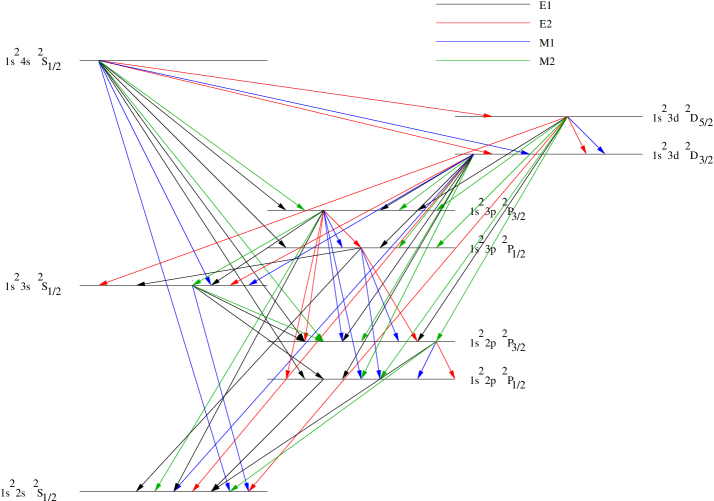
Table 6 presents the comprehensive values of the lifetimes which are compared with the available theoretical data determined by using the non-relativistic multi-configuration Hartree-Fock (MCHF) calculations by Charlotte F. Fischer’s group [8]. We have calculated all possible decay rates of the excited states presented in figure 1. Our calculated lifetimes are in good agreement with Froese Fischer’s data except for the state which is dominated by the electric dipole allowed () decay to the state (given by decay in table 5). In the present calculation we have considered all possible excitations of the core electrons to the virtual apace. This leads to a complete treatment of correlation effects in a more elegant and compact way. Higher order excitations are also taken into account through perturbative triple excitations which we have applied earlier and can be found in Refs. [16, 10]. Inclusion of higher order multipoles leads to the most accurate transition probability data sets of O VI to our knowledge.
| States | Lifetimes (in ) | |
|---|---|---|
| RCCM | MCHF | |
| 2.44 95(-9) | 2.44 60(-9) | |
| 2.40 68(-9) | 2.40 43(-9) | |
| 5.87 37(-11) | 5.85 46(-11) | |
| 3.86 88(-11) | 3.78 54(-11) | |
| 3.88 05(-11) | 3.81 14(-11) | |
| 1.14 20(-11) | 1.14 09(-11) | |
| 1.14 06(-11) | 1.14 23(-11) | |
| 11.04 55(-11) | 9.06 23(-11) | |
Branching ratio of any decay of a particular state depends on the decay probability of that state to all the lower states and is defined as
| (12) |
We have analyzed the branching ratio of the state to different lower states which decay dominantly via electric dipole () transition. The transition rates are given in table 2. Table 7 contains our calculated value of and the comparison with other available data. In the present calculation, the denominator in Eq. (12) consists of the decay rates of the upper state () to the lower states via all possible allowed and forbidden channels, whereas in the other theoretical calculations only allowed transitions have been considered. To show the accuracy of our calculation we have presented the results upto sixth decimal places. Our calculated values of the branching ratios are off by 0.3% - 1.9% as compared to the observed value [18]. Among these transitions, the particular decay () is the dominant one which is within an error of 0.3%. Similarly the branching ratios of decay of the other states can be easily obtained from this work and will be very useful for astrophysical and related studies.
| Methods | ||||
|---|---|---|---|---|
| RCCM | 0.394 548 | 0.196 737 | 0.275 143 | 0.133 610 |
| MCHF | 0.398 581 | 0.199 117 | 0.267 757 | 0.134 543 |
| GRASP | 0.394 314 | 0.196 928 | 0.272 695 | 0.136 063 |
| CIV3 | 0.396 040 | 0.196 220 | 0.271 827 | 0.135 914 |
| NIST | 0.395 985 | 0.198 905 | 0.270 073 | 0.135 036 |
3.1 Order of magnitude estimation
Following Landau and Lifshitz [17] the magnetic moment of an atom is equal in order of magnitude to the Bohr magneton with all the variables with their usual meaning. This differs by a factor of , the fine structure constant, from the order of magnitude of the electric dipole moment . Since , we have approximated . Hence it follows that the probability of radiation from the atom is about times less than the electric dipole () radiation at the same frequency. Magnetic radiation is therefore important in practice only for forbidden transitions governed by the selection rules for the electric case. The ratio of to that of radiation in order of magnitude for a given transition frequency is
| (13) |
where is the change in energy in the transition involved and the order of magnitude of the quadrupole moment and the energy of the atom () are and respectively. For medium atomic transition frequencies () the probabilities of and are of the same order of magnitude. If, however, , i.e. for transitions between two fine structure components of the same term the transition probability is more probable than that of . The results presented in table 3 and 4 and in the figures 3 and 4 follow the pattern.


4 Conclusion
In this paper we have performed relativistic coupled-cluster calculations of all possible allowed and forbidden radiative transition probabilities of the first eight excited states of O VI to the ground state. The lifetimes of those excited states have been determined considering all possible decay channels. This paper reports the first and most comprehensive calculation of the forbidden transition probabilities to our knowledge. Comparison with other available data are made for allowed transitions and radiative lifetimes. Accuracy of the computed transition data depends on both the accuracy of the state energies (transition energies) and the line strengths. Hence the determination of the state energies with an error of (and less than) 2% are used to benchmark the RCCM theory. We also made graphical analysis of the energy dependencies of the and transition probabilities and discussed the trends of different transitions with order of magnitude estimates. We believe that the present data sets will be useful for astrophysical studies of stellar spectra.
Acknowledgment : These computations are carried out in the Intel Xeon cluster at the Department of Astronomy, OSU under the Cluster-Ohio initiative. This work was partially supported by the National Science Foundation and the Ohio State University (CS). RKC acknowledges the Department of Science and Technology, India (grant SR/S1/PC-32/2005). We gratefully acknowledge Prof. Russell Pitzer and Prof. Anil Pradhan for their comments and criticism on the manuscript.
References
- [1] W. A. Feibelman, Astrophys. J. Suppl., 109, 481 (1997).
- [2] W. A. Feibelman, Astrophys. J. Suppl., 114, 263 (1998).
- [3] W. A. Feibelman, Astrophys. J. Suppl., 119, 197 (1998).
- [4] S. S. Tayal, Astrophys. Journal (ApJ), 582, 550 (2003).
- [5] K. M. Aggarwal and F. P. Keenan, Physica Scripta, 70, 222 (2004).
- [6] K. G. Dyall et al, Compt. Phys. Commn., 55, 424 (1989).
-
[7]
S. Ait-Tahar, I. P. Grant, and P. H. Norrington, Phys.
Rev. A, 54, 3984 (1996),
DARC webpage : http://web.am.qub.ac.uk/DARC/ - [8] C. Froese Fischer, M. Sarapov and G. Gaigalas, At. Data and Nuc. Data Tables., 70, 119 (1998).
- [9] R. J. Bartlett, Ann. Rev. Phys. Chem., 32, 359 (1981).
- [10] U. Kaldor, Recent Advances in Coupled-Cluster Methods, p.125, Ed. Rodney J. Bartlett, World Scientific, Singapore (1997) and references therein.
- [11] I. Lindgren and J. Morrison, Atomic Many-Body Theory, Springer Verlag, Berlin (1985).
- [12] B. P. Das et al, Jour. of Theor. Comp. Chem., 4, 1 (2005) and references therein.
- [13] R. K. Chaudhuri, P. K. Panda and B. P. Das, Phys. Rev. A, 59, 1187 (1999).
- [14] B. R. Espey et al, ApJ, 454, L61 (1995).
- [15] M. Hurwitz et al, ApJ, 500, L61 (1998).
- [16] K. Raghavachari, G. W. Trucks, J. A. Pople, M. Head-Gordon, Chem. Phys. Lett., 157, 479 (1989); M. Urban, J. Noga, S. J. Cole and R. J. Bartlett, 83, 4041 (1985).
- [17] L. D. Landau and E. M. Lifshitz, Relativistic Quantum Theory , vol 4, part 1, Pergamon Press, London, (1971).
- [18] National Institute for Science and Technology (NIST) : http://www.nist/gov