Transport through a double barrier in Large Radius Carbon Nanotubes in the presence of a transverse magnetic field

Abstract

We discuss the Luttinger Liquid behaviour of Large Radius Carbon Nanotube e.g. the Multi Wall ones (MWNT), under the action of a transverse magnetic field $B$. Our results imply a reduction with $B$ in the value of the $bulk$ critical exponent, $\alpha_{bulk}$, for the tunneling density of states, which is in agreement with that observed in transport experiments.

Then, the problem of the transport through a Quantum Dot formed by two intramolecular tunneling barriers along the MWNT, weakly coupled to Tomonaga-Luttinger liquids is studied, including the action of a strong transverse magnetic field $B$. We predict the presence of some peaks in the conductance G versus $B$, related to the magnetic flux quantization in the ballistic regime (at a very low temperature, $T$) and also at higher $T$, where the Luttinger behaviour dominates. The temperature dependence of the maximum $G_{max}$ of the conductance peak according to the Sequential Tunneling follows a power law, $G\propto T^{\gamma_{e}-1}$ with $\gamma_{e}$ linearly dependent on the critical exponent, $\alpha_{end}$, strongly reduced by $B$.

I Introduction

In a recent papernoiqw we discussed the transport through a double barrier for interacting quasi one-dimensional electrons in a Quantum Wire (QW), in the presence of a transverse magnetic field. Here we want to extend the results obtained there to an analogous device based on Large Radius Carbon Nanotubes (LRCN), such as the Multi Wall ones (MWNT). This aim is not trivial to pursue, because of the geometry-dependent electronic properties of Carbon Nanotubes (CNs) and the effects of many subbands crossing the Fermi level in LRCNs.

Transport in 1 Dimension - Electronic correlations have been predicted to dominate the characteristic features in quasi one dimensional (1D) interacting electron systems. This property, commonly referred to as Tomonaga-Luttinger liquid (TLL) behaviourTL , has recently moved into the focus of attention by physicists, also because in recent years several electrical transport experiments for a variety of 1D devices, such as semiconductor quantum wireswires (QWs) and carbon nanotubes (CNs)cnts have shown this behaviour.

In a 1D electron liquid Landau quasiparticles are unstable and the low-energy excitations take the form of plasmons (collective electron-hole pair modes): this is known as the breakdown of the Fermi liquid picture in 1D. The LL state has two main features: i) the power-law dependence of physical quantities, such as the tunneling density of states (TDOS), as a function of energy or temperature; ii) the spin-charge separation: an additional electron in the LL decays into decoupled spin and charge wave packets, with different velocities for charge and spin. It follows that 1D electron liquids are characterized by the power-law dependence of some physical quantities as a function of the energy or the temperature. Thus the tunneling conductance $G$ reflects the power law dependence of the DOS in a small bias experimentkf

$$G=dI/dV\propto T^{\alpha_{bulk}}$$ (1)

for $eV_{b}\ll k_{B}T$, where $V_{b}$ is the bias voltage, $T$ is the temperature and $k_{B}$ is Boltzmann’s constant.

The power-law behaviour characterizes also the thermal dependence of $G$ when an impurity is present along the 1D devices. The theoretical approach to the presence of obstacles mixes two theories corresponding to the single particle scattering (by a potential barrier $V_{B}({\bf r})$) and the TLL theory of interacting electrons. The single particle scattering gives the transmission, probability, $|t|^{2}$, depending in general on the single particle energy $\varepsilon$. Hence, following ref.sh , the conductance, $G$, as a function of the temperature and $|t|$ can be obtained

$$G\propto|t(\varepsilon,T)|^{2}\equiv|t(\varepsilon)|^{2}T^{2\alpha_{end},}$$ (2)

where we introduced a second critical exponent, $\alpha_{end}$.

Intrinsic Quantum Dot - ExperimentsPostma01 ; Bozovic01 show transport through an intrinsic quantum dot (QD) formed by a double barrier within a 1D electron system, allowing for the study of the resonant or sequential tunneling. The linear conductance typically displays a sequence of peaks, when the gate voltage, $V_{g}$, increases. Thus also the double-barrier problem has attracted a significant amount of attention among theoristsSassetti95 ; Furusaki98 ; Braggio00 ; Thorwart02 ; Nazarov03 ; Polyakov03 ; Komnik03 ; Hugle04 , in particular for the case of two identical, weakly scattering barriers at a distance $d$. In general, the transmission is non-zero for particular values of the parameters corresponding to a momentum $k_{F}$, such that $\cos(k_{F}d/2)=0$. It follows that, although in a 1D electron system for repulsive interaction the conductance is suppressed at zero temperature by the presence of one impurity (1D metal becomes a perfect insulator), the presence of an intrinsic QD gives rise to some peaks in the conductance at $T=0$ corresponding to the perfect transmission. This resonant scattering condition corresponds to an average particle number between the two barriers of the form $\nu+1/2$, with integer $\nu$, i.e. the “island” between the two barriers is in a degenerate state. If interactions between the electrons in the island are included, one can recover the physics of the Coulomb blockadekf ; furusaki_double_barriere .

The power-law behaviour characterizes also the thermal dependence of $G$ in the presence of an IQD. A first theory about the transport through an IQD is known as Uncorrelated Sequential Tunneling (UST), where an incoherent sequential tunneling is predicted. It follows the dependence of the peaks of the conductance according to the power law

$$G_{max}\propto T^{\alpha_{end}-1}.$$

Some experimentsPostma01 ; Bozovic01 showed transport through an intrinsic quantum dot (QD) formed by a double barrier within a Single Wall CN (SWNT), allowing one to study the resonant or sequential tunneling. In order to explain the unconventional power-law dependencies in the measured transport properties of a CN, a mechanism was proposedPostma01 ; Thorwart02 , namely, correlated sequential tunneling (CST) through the island. The temperature dependence of the maximum $G_{max}$ of the conductance peak, according to the CST theory, yields the power law behaviour

$$G_{max}\propto T^{\alpha_{end-end}-1}=T^{2\alpha_{end}-1}.$$ (3)

Recently a lot of theoretical work has been carried out on the double impurity problem in TLL systems. In an intermediate temperature range $\varepsilon_{c}\ll k_{B}T\ll\Delta_{dot}$, where $\varepsilon_{c}$ is the Infra Red cut-off energy and $\Delta_{dot}$ is the level spacing of the dot, some authorsNazarov03 ; Polyakov03 predict a behaviour according to the UST, while othersHugle04 find results in agreement with the CST theory. In a recent papermeden the authors discussed how the critical exponent can depend on the size of the dot and on the temperature, by identifying three different regimes, i.e. the UST at low $T$, a Kirchoff regime at intermediate $T$ ($G_{max}\propto T^{2\alpha_{end}}$) and a third regime for $T\gg\Delta_{dot}$, with $G_{max}\propto T^{-1}$. Thus, in their calculations, obtained starting from spinless fermions on the lattice model, no evidence of CST is present.

Multi Wall Carbon Nanotubes - An ideal Single Wall CN (SWCN) is an hexagonal network of carbon atoms (graphene sheet) that has been rolled up, in order to make a cylinder with a radius about $1nm$ and a length about $1\mu m$. The unique electronic properties of CNs are due to their diameter and chiral angle (helicity)3n . MWCNs, instead, are made by several (typically 10) concentrically arranged graphene sheets with a radius above $5nm$ and a length which ranges from $1$ to some hundreds of $\mu m$s. The transport measurements carried out in the MWNTs reflect usually the electronic properties of the outer layer, to which the electrodes are attached. Thus, in what follows we mainly discuss the LRCNs as a general class of CNs including also MWNTs. In general the LRCNs are affected by the presence of doping, impurities, or disorder, what leads to the presence of a large number of subbands, $N$, at the Fermi level[21] . It follows that the critical exponent has a different form with respect to that calculated in ref.noiqw .

The bulk critical exponent can be calculated in several different ways, e.g. see ref.npb where we obtained

$$\alpha_{bulk}\approx\frac{1}{4N}\left(K_{N}+\frac{1}{K_{N}}-2\right),$$ (4)

where

$$\frac{1}{K_{N}}\approx\sqrt{1+\frac{NU_{0}(q_{c},B)}{(2\pi{v}_{F})}}.$$

Here $v_{F}$ is the Fermi velocity, $U_{0}(p)$ corresponds to the Fourier transform of the 1D e-e interaction potential and $q_{c}=2\pi/L$ is the infra-red natural cut-off due to the length of the CN, $L$. For a strictly 1D system, such as a CN in absence of magnetic field, $U_{0}(p)$ does not depend on the momenta of the interacting electrons. In generalnoiqw0 we need to introduce two different couplings for two different forward scattering processes (with a small transferred momentum). The first term, $g_{2}$, is obtained by considering $2$ scattered electrons with opposite momenta ($\pm k_{F}$). The second term, $g_{4}$, is obtained by considering $2$ scattered electrons with (almost) equal momenta ($k_{1}\sim k_{2}\sim k_{F}$). It follows that

$${K_{N}}\approx\sqrt{\frac{2\pi{v}_{F}+N\left(g_{4}-g_{2}\right)/2}{2\pi{v}_{F}+N\left(g_{4}+g_{2}\right)/2}},$$

which corresponds to the previous formula when $g_{2}=g_{4}=U_{0}(q_{c})$. As in ref.noiqw0 the presence of a magnetic field gives $g_{2}\neq g_{4}$, because of the edge localization of the currents with opposite chiralities, and we need the $B$ dependent values of $g_{2}$ and $g_{4}$.

The value of $\alpha_{bulk}$ obtained in refnpb is in agreement with the one obtained in ref.egmw where also the end critical exponent was obtained as

$$\alpha_{end}\approx\frac{1}{2N}\left(\frac{1}{K_{N}}-1\right).$$ (5)

Power law in MWNTs -One of the most significant observations made in the MWNTs has been the power-law behavior of the tunneling conductance as a function of the temperature or the bias voltage. The measurements carried out in the MWNTs have displayed a power-law behavior of the tunneling conductance, that gives a measure of the low-energy density of states. Although the power law behaviour in the temperature dependence of $G$ usually characterizes a small range of temperature (from some $-K$ up to some tens, rarely up to the room $T$), this behaviour allows for the measurement of the critical exponent $\alpha_{Bulk}$ ranging, in MWNTs, from $0.24$ to $0.37$B . These values are, on the average, below those measured in single-walled nanotubes, which are typically about $0.35$ y . A similar behaviour was satisfactory explainednpb in terms of the number of subbands by applying eq.(4).

CNs under a transverse magnetic field - The effects of a transverse magnetic field $B$, acting on CNs were also investigated in the last years. Theoretically, it is predicted that a perpendicular $B$ field modifies the DOS of a CN [33] , leading to the Landau level formation. This effect was observed in a MWNT single-electron transistor [34] . In a recent letter Kanda et al.kanda examined the dependence of $G$ on perpendicular $B$ fields in MWNTs. They found that, in most cases, $G$ is smaller for higher magnetic fields, while $\alpha_{Bulk}$ is reduced by a factor $1/3$ to $1/10$, for $B$ ranging from $0$ to $4$ T. Recently we discussed the effects of a transverse magnetic field in QWsnoiqw and large radius CNsnoimf . The presence of $B\neq 0$ produces the rescaling of all repulsive terms of the interaction between electrons, with a strong reduction of the backward scattering, due to the edge localization of the electrons. Our results imply a variation with $B$ in the value of $\alpha_{Bulk}$, which is in fair agreement with the value observed in transport experimentskanda .

Impurities, buckles and Intrinsic QD - The magnetic induced localization of the electrons should have some interesting effects also on the backward scattering, due to the presence of one or more obstacles along the LRCN, and hence on the corresponding conductance, $G$noiqw . Thus, the main focus of our paper is to analyze the presence of two barriers along a LRCN at a fixed distance $d$. A similar device was made by the manipulation of individual nanotubes with an atomic force microscope which permitted the creation of intratube buckles acting as tunneling barriersPostma01 . The SWNTs with two intramolecular buckles have been reported to behave as a room-temperature single electron transistor. The linear conductance typically displays a sequence of peaks when the gate voltage, $V_{g}$, increases. The one-dimensional nature of the correlated electrons is responsible for the differences to the usual quantum Coulomb blockade theory.

We predict that, in the presence of a transverse magnetic field, a LRCN should show some oscillations in the conductance as a function of the magnetic field, like those discussed in ref.noiqw .

Summary - In this paper we want to discuss the issues mentioned above. In order to do that we follow the same structure of our previous papernoiqw .

In section II we introduce a theoretical model which can describe the CN under the effect of a transverse magnetic field, and we discuss the properties of the interaction starting from the unscreened long range Coulomb interaction in two dimensions.

In section III we evaluate the $bulk$ and $end$ critical exponents. Then we discuss the effects on them due to an increasing transverse magnetic field. We remark that $\alpha_{bulk}$ characterizes the discussed power-law behavior of the TDOS, while ($\alpha_{end}$) characterizes the temperature dependence of $G_{max}$, in both the UST and the CST regime. Finally, we discuss the presence of an intrinsic QD and the magnetic field dependent oscillations in the conductance.

II Model and Interaction

Single particle - Starting from the known bandstructure of graphite, after the definition of the boundary condition (i.e. the wrapping vector $\overrightarrow{w}=(m_{w},n_{w})$), it is easy to calculate the bandstructure of a CN. For an armchair CN ($m_{w}=n_{w}$) we obtain that the energy vanishes for two different values of the longitudinal momentum $\varepsilon_{0}(\pm K_{s})=0$. After fixing the angular momentum along the $y$ direction to be $m\hbar$, the dispersion law $\varepsilon_{0}({m},k)$ is usually taken to behave linearly, so that we can approximate it as $\varepsilon_{0}({m},k)\approx\varepsilon_{0}({m},K_{s})+v_{F}|k-K_{s}|$, where we introduce a Fermi velocity $v_{F}$ (about $10^{6}\,m/s$ for CNs). In general, we can define an approximate one-dimensional bandstructure for momenta near $\pm K_{s}=\pm(2\pi)/(3a_{0})$

$$\varepsilon_{0}({m},\overrightarrow{w},k)\approx\pm\frac{v_{F}\hbar}{R}\sqrt{\left(\frac{m_{w}-n_{w}+3m}{3}\right)^{2}+R^{2}\left(k\pm K_{s}\right)^{2}}$$ (6)

where $R\approx N_{b}\sqrt{3}a/(2\pi)$ is the tube radius (about $5\,nm$ for MWNTs) and $a$ denotes the honeycomb lattice constant ($a/\sqrt{3}=a_{0}=1.42\AA$).

For a metallic CN (e.g. the armchair one with $m_{w}=n_{w}$) we obtain that the energy vanishes for two different values of the longitudinal momentum $\varepsilon_{0}(\pm K_{s})=0$. The dispersion law $\varepsilon_{0}({m},k)$ in the case of undoped metallic nanotubes is quite linear near the crossing values $\pm K_{s}$. The fact of having four low-energy linear branches at the Fermi level introduces a number of different scattering channels, depending on the location of the electron modes near the Fermi points.

Starting from eq.(6) we can develop a Dirac-like theory for CNs corresponding to the hamiltonian

$$H_{D}=v_{F}\left[\widehat{\alpha}(\hat{L}_{z})+\widehat{\beta}\hat{\pi}_{y}\right],$$ (7)

with a solution in the spinorial form $\widehat{\psi}$ where

$$\widehat{\alpha}=\alpha\left(\begin{array}[]{cc}0&i\\ -i&0\end{array}\right)\;\;\;\widehat{\beta}=\left(\begin{array}[]{cc}0&1\\ 1&0\end{array}\right)\;\;\;\widehat{\Psi}=\left(\begin{array}[]{c}\psi_{\uparrow}\\ \psi_{\downarrow}\end{array}\right).$$ (14)

Here $\hat{\pi}_{y}=\hat{p}_{y}\pm\hbar K_{s}$, and $\alpha=\frac{1}{R^{2}}$, and eq.(7) can be compared with the one obtained in refsusy .

For the metallic CN, such as the armchair one, the problem in eq.(7) has periodic boundary conditions i.e. $\Psi(\varphi+2\pi,y)=\Psi(\varphi)$, it follows that a factor $e^{im\varphi}$ appears in the wavefunction. For semiconducting CNs ($m_{w}\neq n_{w}$) we have to define quasiperiodic boundary conditions i.e. $\Psi(\varphi+2\pi,y)=\omega\Psi(\varphi)$susy corresponding to a factor $e^{i(m+\frac{m_{w}-n_{w}}{3}\varphi)}$ in the wavefunction ($m_{0}=m_{w}-n_{w}$).

A cylindrical carbon nanotube with the axis along the $y$ direction and $B$ along $z$ corresponds to

$$H_{D}=v_{F}\left[\widehat{\alpha}(\hat{L}_{z})+\widehat{\beta}\left(\hat{\pi}_{y}-\frac{e}{c}{\bf A}\right)\right],$$ (15)

where we choose the gauge so that the system has a symmetry along the $\hat{y}$ direction,

$${\bf A}=(0,Bx,0)=(0,BR\cos(\varphi),0)$$

and we introduce the cyclotron frequency $\omega_{c}=\frac{eB}{m_{e}c}$ and the magnetic length $\ell_{\omega}=\sqrt{\hbar/(m\omega_{c})}$.

It is usual to discuss the results in terms of two parameters, one for the scale of the energy following from eq.(6)

$$\Delta_{0}={\hbar v_{F}\over R}\ ,$$ (16)

the second one being the scale of the magnetic field

$$\nu\equiv{\pi R^{2}\over 2\pi\ell_{\omega}^{2}}={\pi R^{2}B\over\Phi_{0}}\quad where\quad\Phi_{0}={hc\over e}.$$ (17)

Here we can calculate the effects of the magnetic field by diagonalizing eq.(15), after introducing the trial functions

$$\widetilde{\psi}_{s,m,k}(\varphi,y)=Ne^{i\left(ky+(m+m_{0})\varphi\right)}\left(\alpha_{s}+\beta_{s}\sin(\varphi)+\gamma_{s}\cos(\varphi))\right).$$ (18)

Results are reported in Fig.(1) for different CNs and values of the magnetic field.

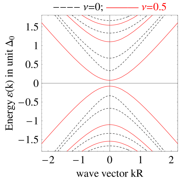
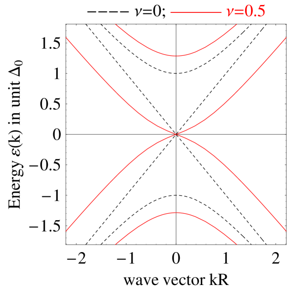
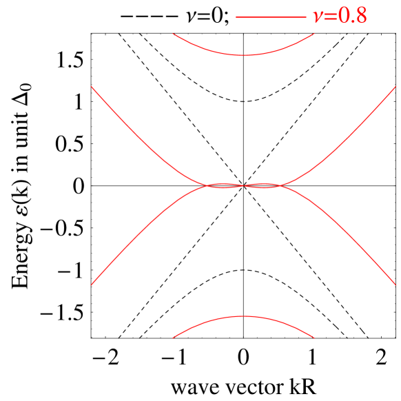
Figure 1: In the x-axis the wavevector in unit $(k_{y}-K_{s})R$ ($\pi_{y}R/\hbar$). (Top) Bandstructure of a non-metallic CN with (red lines) and without (black dashed lines) the transverse magnetic field ($\nu=0.5$). The main consequence of $B$ is the reduction of the semiconducting gap. (Middle and bottom) Bandstructure of a metallic CN with (red lines) and without (black dashed lines) the transverse magnetic field. The main consequence of $B$ at intermediate fields is the rescaling of the Fermi velocity, while for quite strong fields a flat zone appears near $\pi_{y}=0$. We know that the magnetic parameter $\nu\approx 0.2$ for $B\sim 5\,T$ and $R\approx 50nm$andos .

From the expression of $|{\Psi}_{m,\pm k}(\varphi,y)|^{2}$ we deduce a kind of ”edge localization” of the opposite current, analogous to the one obtained for the QWnoiqw also for CNs.

Following the calculations reported in ref.(susy ) for a metallic CN we can easily calculate the linear dispersion relation changes near the band center $\epsilon=0$. Thus, the magnetic dependent energy can be written, near the Fermi points $k\sim K_{s}$, in terms of $\nu$ as

$$\epsilon(|k-K_{s}|)=\pm\hbar|k-K_{s}|\left({v_{F}\over I_{0}(4\nu)}\right)\ .$$ (19)

This describes a reduction of the Fermi velocity $\hbar^{-1}d\epsilon/dk$ near $\epsilon=0$ by a factor $I_{0}(4\nu)$.

Hence, the magnetic dependent Fermi wavevector follows

$$k_{F}(\varepsilon_{F},\nu,0)\approx K_{s}+\left(\frac{\varepsilon_{F}}{\hbar v_{F}}\right)I_{0}(4\nu),$$

where the second term in the r.h.s. depends on $B$ as

$$k_{F}=K_{s}\pm k_{0}+k(B)\approx K_{s}\pm k_{0}(1+4\nu^{2}+...)\rightarrow k(B)\sim 4k_{0}\nu^{2},$$

where $k_{0}=\left(\frac{\varepsilon_{F}}{\hbar v_{F}}\right)$.

Electron-electron interaction -

In order to analyze in detail the role of the e-e interaction, we have to point out that quasi 1D devices have low-energy branches, at the Fermi level, that introduce a number of different scattering channels, depending on the location of the electron modes near the Fermi points. It has been often discussed that processes which change the chirality of the modes, as well as processes with large momentum-transfer (known as backscattering and Umklapp processes), are largely subdominant, with respect to those between currents of like chirality (known as forward scattering processes)8n ; 9n ; egepj . This hierarchy of the couplings characterizes the Luttinger regime. However in some special cases the processes neglected here can be quite relevant, giving rise even to a breakdown of the Luttinger Liquid behaviournoisc .

Now, following Egger and Gogolinegepj , we introduce the unscreened Coulomb interaction in two dimensions

$$U({\bf r}-{\bf r^{\prime}})=\frac{c_{0}}{\sqrt{(y-y^{\prime})^{2}+4R^{2}\sin^{2}(\frac{\varphi-\varphi^{\prime}}{2})}}.$$ (20)

Then, we can calculate $U_{0}(q,\omega_{c})$ starting from the eigenfunctions $\widetilde{\Psi}_{0,k_{F}}(\varphi,y)$ and the potential in eq.(20). We focus our attention on the forward scattering (FS) terms. We can obtain $g_{2}$, FS between opposite branches, corresponding to the interaction between electrons with opposite momenta, $\pm k_{F}$, with a small momentum transfer $\sim q_{c}$. The strength of this term reads

$$g_{2} = U_{0}(q_{c},B,k_{F},-k_{F})$$

$$= \frac{c_{0}}{N_{2}(\nu)}\left[K_{0}(\frac{q_{c}R}{2})I_{0}(\frac{q_{c}R}{2})+u_{2}(\nu)K_{1}(\frac{q_{c}R}{2})I_{1}(\frac{q_{c}R}{2})\right],$$

where $K_{n}(q)$ denotes the modified Bessel function of the second kind, $I_{n}(q)$ is the modified Bessel function of the first kind, while $N_{2}$ and $u_{2}$ are functions of the transverse magnetic field, as we discuss in appendix. Analogously

$$g_{4} = U_{0}(q_{c},B,k_{F},k_{F})$$

$$= \frac{c_{0}}{N_{4}(\nu)}\left[K_{0}(\frac{q_{c}R}{2})I_{0}(\frac{q_{c}R}{2})+u_{4}(\nu)K_{1}(\frac{q_{c}R}{2})I_{1}(\frac{q_{c}R}{2})\right].$$

III Results

The bulk and the end critical exponents - The first result of this paper concerns the dependence of the critical exponents on the magnetic field, in large radius CNs. By introducing into eq.(4) the calculated values of $g_{2}$ and $g_{4}$, it follows that the bulk critical exponent is reduced by the presence of a magnetic field, as we show in Fig.(2).

Figure 2: Critical exponents versus the magnetic field dependent parameter, $\nu$, for a large radius CN: $\alpha_{bulk}$ is calculated following eq.(4), $\alpha_{end}$ is calculated following eq.(5).The magnetic field rescales the values of the Fermi velocity and the strength of e-e interaction. It follows that the effects of a transverse magnetic field also involve the value of $K$. Thus, we predict a reduction of the critical exponents $\alpha_{bulk}$ and $\alpha_{end}$, by giving magnetic field dependent exponents for the power law behaviour of the conductance.

This prediction can be extended to $\alpha_{end}$, calculated following eq.(5), as we show in Fig.(2). Hence, it follows that the exponent $\gamma_{e}-1$ can cross from positive to negative values, when the magnetic field increases.

The experimental data about SWNTPostma01 gives, for vanishing magnetic field, $K_{1}\approx 0.26$, $\alpha_{Bulk}\approx 0.27$ and $\alpha_{end}\approx 0.72$.

For a MWNT we consider $N_{s}\sim 5$kanda ; noiprl so that $K_{5}\approx 0.1$, $\alpha_{Bulk}\approx 0.2$ and $\alpha_{end}\approx 0.4-0.5$.

The intrinsic Quantum Dot - When there are some obstacles to the free path of the electrons along a 1D device, a scattering potential has to be introduced in the theoretical model. The presence of two barriers along a CNPostma01 at a distance $d$ can be represented by a potential

$$V_{B}(y)=U_{B}\left(f(y+\frac{d}{2})+f(y-\frac{d}{2})\right),$$

where $f(y)$ is a square barrier function, a Dirac Delta function or any other function localized near $y=0$. In general we can analyze the single particle transmission in the presence of a magnetic field, $t(\varepsilon_{F},B)$, by identifying the off-resonance condition ($|t|=0$), where electrons are strongly backscattered by the barriers, and the on-resonance condition ($|t|=1$), where the scattering at low temperatures is negligible.

Hence, as shown in Fig.(3), where we report the transmission $T=|t|^{2}$ versus $\nu$ for the lowest subband, a magnetic field dependent transmission follows, thus a magnetic dependence of the peaks in the transmission is shown which exhibits a magnetically tuned transport through the CN. In particular, assuming that there are two identical, weakly scattering barrier at a distance $d$, the transmission is non-zero for particular values of $k_{F}$, so that $\cos(k_{F}d)\approx 0$.

Figure 3: Transmission ($T$) of the lowest subband ($m=0$) as a function of the magnetic field. We use a double square barrier model, for the IQD. We observe the appearing of resonance peaks, as a function of the magnetic field. The ballistic conductance (at very low temperatures) is proportional to $|t|^{2}$ according to the Landauer formula.

We consider an intrinsic QD with $d\approx 250nm$ in a CN of $R\approx 5nm$. Thus, starting from the electrons in the middle of the bandgap, i.e. $\varepsilon_{F}\sim v_{F}\hbar/(2R)$, $k(B)\approx\nu^{2}/(2R)$, we have to observe about $4$ peaks (i.e. the number of resonances with $\nu\leq 1$ is $n_{p}=d/(4\pi R)$) in the transmission, when growing the magnetic field from $\nu=0$ to $\nu=1$.

The presence of these oscillations has to be seen in MWNTs or SWNTs of large radius, while in the case of a SWNTs with radius $R\approx 1nm$ the values of the magnetic field are unrealistic.

Analogously to our previous papernoiqw we can discuss the different explanations of the resonance conditions. From a theoretical point of view the on resonance condition can be seen in two different ways: in some papersvw , where the ballistic transport in QWs was analyzed, it was discussed the presence of these peaks as providing evidence of an Aharonov Bohm effect, while in the TLL theory the resonance peaks are put in correspondence to the presence of an average particle number between the two barriers of the form $\nu+1/2$, with integer $\nu$: thus we suppose that each electron in the QD carries a quantum of magnetic flux.

Temperature behaviour - As it is known the presence of the peaks in the transmission has to be observable not only at very low temperatures. The temperature does not affect the values of $B$ corresponding to the conductance peaks, while their largest value, $G_{max}$, follows a power law according to the Sequential Tunneling theory. Thus, $G_{max}\propto T^{\gamma_{e}-1}$ with $\gamma_{e}$ depending on the tunneling mechanism. This point deserves a brief discussion.

In this paper we take into account a short nanotube section that is created by inducing (e.g. with an atomic force microscope) local barriers into a large radius CN. In this case the condition, $\Delta_{dot}\gg K_{B}T$ discussed in ref.Postma01 is confirmed in a large range of temperatures around $T_{R}$ ($\Delta_{dot}/K_{B}\sim 10^{4}\;{}^{o}K$, while $\varepsilon_{c}/K_{B}\sim 1\;^{o}K$).

Now we could discuss the two cases, by assuming the validity of either the UST or the CST. In any case, we want to point out that in both theories, it appears the critical exponent $\alpha_{end}$, which has to be rescaled with the growing of the magnetic field. The discussed reduction of $\alpha_{end}$, due to the increasing magnetic field, also affects the shape of the peaks.

The intersubbands processes - The role of the many subbands ($N_{s}$) which cross the Fermi level should be taken into account by introducing the matrix $t_{n,m}$ including all the intersubband scattering processes. However we can suppose $|t_{n,m}|\ll|t_{n,n}|$, corresponding to the adiabatic regime, because the intersubbands processes, i.e. the processes that involves two different subbands, are largely subdominants with respect to the processes involving the same subband. It follows that the conductance $G$ results proportional to the sum of the $|t_{n,n}|$. Thus, the peaks corresponding to the on resonance condition, due to the $N_{s}$ subbands have to be superposed in order to calculate the zero temperature conductance. However, the contribution to the oscillations due to the subbands different from the lowest one can be negligible, because the shift in $k(B)$ is quite smaller for the higher subbands, as we show in Fig(1).

IV Conclusions

In this paper we extended to large radius CNs the formalism introduced for a QW in a previous paper. We showed how the presence of a magnetic field modifies the role played by both the e-e interaction and the presence of obstacles in CNs of large radius.

The first prediction that comes from our study is that there should be a significant reduction of the critical exponents, as the magnetic field is increased, in agreement with the results found for QWs.

Our second prediction concerns the presence of some peaks in the small bias conductance versus the magnetic field.

It would be of considerable importance to test this behaviour in experiments carried out using different samples, in various temperature regimes. This experimental test can be also useful, in order to solve the controversial question about the exponent that characterizes the power law dependence of $G(T)$.

We want to remark that our approach is based on the idea that electrons tunnel coherently through an obstacle, represented by a double barrier, that can be assumed only as a strong barrier.

Our results could be surely affected by the use of a model, where the electrons weakly interact with the lattice, while the buckles are represented by strong potential barriers. This approximation holds in the opposite regime, with respect to the model of spinless fermions on the lattice used in ref.meden . However, we believe that our model can well reproduce some experimental results while, for what concerns the different regimes, we want also to suggest that, when the temperature decreases, different approaches could be needed, as we discussed in some of our previous papersnoicb ; noiprl .

Appendix A From the 2D Coulomb potential to a 1D Model

Firstly, we introduce the wavefunctions $\Psi$ for a metallic CN, as spinors constructed starting from the functions

$$\widetilde{\psi}_{s,m,k}(\varphi,y)=\frac{e^{i\left(ky+im\varphi\right)}}{N}\left(\alpha_{s}+\beta_{s}\sin(\varphi)+\gamma_{s}\cos(\varphi))\right),$$

it follows

$$\Psi^{\dagger}\Psi=\frac{\sum_{s=\uparrow,\downarrow}\left((\alpha_{s}^{2}+\beta_{s}^{2})+2(\alpha_{s}\gamma_{s})\cos(\varphi)+(\gamma_{s}^{2}-\beta_{s}^{2})\cos(\varphi)^{2}+\left[2(\alpha_{s}\beta_{s})\sin(\varphi)+(\beta_{s}\gamma_{s})\sin(2\varphi)\right])\right)}{{2\pi^{2}L\sum_{s=\uparrow,\downarrow}(2\alpha_{s}^{2}+\beta_{s}^{2}+\gamma_{s}^{2})}},$$

and we define $\eta_{\pm}=\sum_{s=\uparrow,\downarrow}(\alpha_{s}^{2}+\beta_{s}^{2})$, $\theta_{\pm}=\sum_{s=\uparrow,\downarrow}2(\alpha_{s}\gamma_{s})$, $\xi_{\pm}=\sum_{s=\uparrow,\downarrow}(\gamma_{s}^{2}-\beta_{s}^{2})$ and $N_{\pm}=\sum_{s=\uparrow,\downarrow}(2\alpha_{s}^{2}+\beta_{s}^{2}+\gamma_{s}^{2})$, where $\pm$ corresponds to the values of $k=\pm k_{F}$.

Now we introduce the Coulomb interaction and expand this function in terms of $R/|y-y^{\prime}|$ as

$$U({\bf r}-{\bf r^{\prime}})=\frac{c_{0}}{|y-y^{\prime}|}\left(\sum_{k}^{\infty}\frac{{\left(-1\right)}^{k}\,\,\Gamma(\frac{1}{2}+k)}{{\sqrt{\pi}}\,\Gamma(1+k)}\left(\frac{2R}{y-y^{\prime}}\right)^{2\,k}\sin^{2\,k}(\frac{\varphi-\varphi^{\prime}}{2})\right).$$

The Forward scattering between opposite branches ($\pm$) is obtained as

$$U(y - y^{\prime})\approx c_{0}\int_{-\pi}^{\pi}d\varphi\int_{-\pi}^{\pi}d\varphi^{\prime}\sqrt{\frac{1}{(y-y^{\prime})^{2}+4R^{2}\sin^{2}(\frac{\varphi-\varphi^{\prime}}{2})}}{\Psi^{\dagger}}_{m,k_{F}}(\varphi,y){\Psi}_{m,k_{F}}(\varphi,y){\Psi}_{n,-k_{F}}(\varphi^{\prime},y^{\prime}){\Psi^{\dagger}}_{n,-k_{F}}(\varphi^{\prime},y^{\prime})$$ (21)

$$= \frac{c_{0}}{4\pi^{2}}\int_{-\pi}^{\pi}d\varphi\int_{-\pi}^{\pi}d\varphi^{\prime}\sqrt{\frac{1}{(y-y^{\prime})^{2}+4R^{2}\sin^{2}(\frac{\varphi-\varphi^{\prime}}{2})}}\left(\frac{\eta_{+}+\theta_{+}\cos(\varphi^{\prime})+\xi_{+}\cos^{2}(\varphi^{\prime})}{{N_{+}}}\right)\left(\frac{\eta_{-}+\theta_{-}\cos(\varphi)+\xi_{-}\cos^{2}(\varphi)}{{N_{-}}}\right)$$

$$\approx \frac{c_{0}}{4\pi^{2}}\sqrt{\frac{1}{(y-y^{\prime})^{2}}}\int_{-\pi}^{\pi}d\varphi\int_{-\pi}^{\pi}d\varphi^{\prime}\left(\sum_{k}^{\infty}\frac{{\left(-1\right)}^{k}\,\,\Gamma(\frac{1}{2}+k)}{{\sqrt{\pi}}\,\Gamma(1+k)}\left(\frac{2R}{y-y^{\prime}}\right)^{2\,k}\sin^{2\,k}(\frac{\varphi-\varphi^{\prime}}{2})\right)$$

$$\times \left(\frac{(\eta_{+}\eta_{-}+(\eta_{+}\theta_{-}+\eta_{-}\theta_{+})\,\cos(\varphi)\,\cos(\varphi^{\prime})+(\xi_{+}\cos^{2}(\varphi)+\xi_{-}\cos^{2}(\varphi^{\prime})))}{{\left(N_{+}N_{-}\right)}}\right)$$

$$= \frac{2c_{0}}{N_{+}N_{-}}\sqrt{\frac{1}{(y-y^{\prime})^{2}}}\sum_{n}^{\infty}\frac{{\left(-1\right)}^{n}\,\,\Gamma(\frac{1}{2}+n)}{{\sqrt{\pi}}\,\Gamma(1+n)}\left(\frac{2R}{y-y^{\prime}}\right)^{2\,n}$$

$$\times \left(\left(\eta_{+}\eta_{+}+\frac{\xi_{+}+\xi_{-}}{2}\right)\frac{4\pi^{3/2}\Gamma(n+1/2)}{\Gamma(n+1)}+(\eta_{+}\theta_{-}+\eta_{-}\theta_{+})\frac{2\pi^{3/2}n\Gamma(n+1/2)}{\Gamma(n+2)}\right).$$

Thus, we introduce $u_{0}=\eta_{+}\eta_{-}$,$u_{1}=(\eta_{+}\theta_{-}+\eta_{-}\theta_{+})$and $u_{2}=(\xi_{+}+\xi_{-})$ so that we obtain

$$U(y-y^{\prime}) = 2\frac{c_{0}}{\left(N_{+}N_{-}\right)}\sqrt{\frac{1}{(y-y^{\prime})^{2}}}$$ (22)

$$\times \left\{(u_{0}+\frac{u_{1}}{2})K(-(\frac{2R}{y-y^{\prime}})^{2})+u_{2}\left(\frac{\pi}{8}\,_{2}F_{1}(\frac{3}{2},\frac{3}{2};2,-(\frac{2R}{y-y^{\prime}})^{2})\left[\frac{2R}{y-y^{\prime}}\right]^{2}\right)\right\}$$

Where $K_{E}(x)$ gives the complete elliptic integral of the first kind while ${}_{2}F_{1}(a,b,c,z)$ is the hypergeometric function.

The Fourier Transform gives the $U_{0}(q)$ as

$$U_{0}(q)=\frac{c_{0}}{\sqrt{2}\left(N_{+}N_{-}\right)^{2}}\left[(u_{0}+\frac{u_{1}}{2})K_{0}(\frac{qR}{2})I_{0}(\frac{qR}{2})+\frac{u_{2}}{2}K_{1}(\frac{qR}{2})I_{1}(\frac{qR}{2})\right]$$ (23)

with $K_{n}(q)$ which gives the modified Bessel function of the second kind and $I_{n}(q)$ gives the modified Bessel function of the first kind.

In order to calculate $g_{4}$ we have to define $u_{0}=\eta_{+}^{2}$,$u_{1}=2\eta_{+}\theta+$ and $u_{2}=2\xi_{+}$, and then plug these expressions in the equations above.

References

- (1) S. Bellucci and P. Onorato, Eur. Phys. J. B 47, 385-390 (2005).
- (2) S. Tomonaga, Prog. Theor. Phys. 5, 544 (1950); J. M. Luttinger, J. Math. Phys. 4, 1154 (1963); D. C. Mattis and E. H. Lieb, J. Math. Phys. 6, 304 (1965).
- (3) A. Yacoby, H. L. Stormer, N. S. Wingreen, L. N. Pfeiffer, K. W. Baldwin and K. W. West, Phys. Rev. Lett. 77, 4612 (1996); O. M. Auslaender, A. Yacoby, R. de Picciotto, K. W. Baldwin, L. N. Pfeiffer and K. W. West, Phys. Rev. Lett. 84, 1764 (2000),
- (4) S. J. Tans, M. H. Devoret, H. Dai, A. Thess, R. E. Smalley, L. J. Geerligs and C. Dekker, Nature 386, 474 (1997);Z. Yao, H. W. J. Postma, L. Balents, and C. Dekker, Nature 402, 273 (1999).
- (5) C. L. Kane and M. P. A. Fisher, Phys. Rev. Lett. 68, 1220 (1992); C. L. Kane and M. P. A. Fisher, Phys. Rev. B 46, R7268 (1992)
- (6) H. J. Schulz, cond-mat/9503150.
- (7) H.W.Ch. Postma, T. Teepen, Z. Yao, M. Grifoni, and C. Dekker, Science 293, 76 (2001).
- (8) D. Bozovic, M. Bockrath, J.H. Hafner, C. M. Lieber, H. Park, and M. Tinkham, Appl. Phys. Lett. 78, 3693 (2001).
- (9) M. Sassetti, F. Napoli, and U. Weiss, Phys. Rev. B 52, 11213 (1995).
- (10) A. Furusaki, Phys. Rev. B 57, 7141 (1998).
- (11) A. Braggio, M. Grifoni, M. Sassetti, and F. Napoli, Europhys. Lett. 50, 236 (2000).
- (12) M. Thorwart, M. Grifoni, G. Cuniberti, H.W.Ch. Postma, and C. Dekker, Phys. Rev. Lett. 89, 196402 (2002).
- (13) Yu.V. Nazarov and L.I. Glazman, Phys. Rev. Lett. 91, 126804 (2003).
- (14) D.G. Polyakov and I.V. Gornyi, Phys. Rev. B 68, 035421 (2003).
- (15) A. Komnik and A.O. Gogolin, Phys. Rev. Lett. 90, 246403 (2003).
- (16) S. Hügle and R. Egger, Europhys. Lett. 66, 565 (2004).
- (17) A. Furusaki and N. Nagaosa, Phys. Rev. B 47, 3827 (1993).
- (18) V. Meden,T. Enss, S. Andergassen, W. Metzner, and K. Schönhammer, Phys. Rev. B 71, 041302(R) (2005),
- (19) J.W. Mintmire, B.I. Dunlap, C.T. White, Phys. Rev. Lett. 68 (1992) 631; N. Hamada, S. Sawada, A. Oshiyama, Phys. Rev. Lett. 68 (1992) 1579; R. Saito, M. Fujita, G. Dresselhaus, M.S. Dresselhaus, Appl. Phys. Lett. 60 (1992) 2204.
- (20) M. Krüger, M. R. Buitelaar, T. Nussbaumer, C. Schönenberger, and L. Forró, Appl. Phys. Lett. 78, 1291 (2001).
- (21) S. Bellucci, J. González, P. Onorato, Nucl. Phys. B 663 [FS] (2003) 605; S. Bellucci, J. González, P. Onorato, Phys. Rev. B 69 (2004) 085404.
- (22) S. Bellucci and P. Onorato, Eur. Phys. J. B 45, 87-96 (2005).
- (23) R. Egger, Phys. Rev. Lett. 83, 5547 (1999).
-
(24)
A. Bachtold, M. de Jonge, K. Grove-Rasmussen, P. L. McEuen, M.
Buitelaar and C. Sch nenberger, Phys. Rev. Lett. 87,
166801 (2001);
A. Bachtold, M. de Jonge, K. Grove-Rasmussen, P.L. McEuen, M. Buitelaar and C. Schonenberger, report cond-mat/0012262. - (25) Z. Yao, H. W. Ch. Postma, L. Balents and C. Dekker, Nature 402, 273 (1999).
- (26) H. Ajiki and T. Ando, J. Phys. Soc. Jpn. 62, 1255 (1993).
- (27) A. Kanda et al., Physica B, 323, 107-114 (2002).
- (28) A. Kanda, K. Tsukagoshi, Y. Aoyagi and Y. Ootuka, Phys. Rev. Lett. 92, 36801 (2004).
- (29) S. Bellucci and P. Onorato, Annals of Physics 321, 934-949 (2006).
- (30) H.-W. Lee, D. S. Novikov, Phys. Rev. B 68 155402 (2003).
- (31) T. Ando, T. Seri, J. Phys. Soc. Jpn. 66, 3558 (1997).
- (32) L. Balents, M.P.A. Fisher, Phys. Rev. B 55 (1997) R11973.
- (33) R. Egger, A. O. Gogolin, Phys. Rev. Lett. 79 (1997) 5082
- (34) R. Egger, A. O. Gogolin,, Eur. Phys. J. B 3 (1998) 281.
- (35) S. Bellucci, M. Cini ,P. Onorato and E. Perfetto (2006) accepted for publication in Journal of Physics: Condensed Matter cond-mat/0603853.
- (36) B. J. van Wees, H. van Houten, C. W. J. Beenakker, J. G. Williamson, L. P. Kouwenhoven, D. van der Marel and C. T. Foxon,, Phys. Rev. Lett. 60, 848 (1988).
- (37) S. Bellucci and P. Onorato, Phys. Rev. B 71, 075418 (2005).
- (38) S. Bellucci, J. González, P. Onorato, Phys. Rev. Lett. 95, 186403 (2005).