Dynamics of wave packets in two-dimensional crystals under external magnetic and electric fields: Vortices formation

Abstract

In the present work we deal with the dynamics of wave packets in a two-dimensional crystal under the action of magnetic and electric fields. The magnetic field is perpendicular to the plane and the electric field is on the plane. In the simulations we considered a symmetric gauge for the vector potential while the initial wave packet was assumed to have a gaussian structure with given velocities. The parameters that control the kind of time evolution of the packets are: the width of the gaussian, its velocity, and, the intensity and direction of the electric field as well as the magnitude of the magnetic field. In order to characterize the kind of propagation we evaluated the mean-square displacement (MSD), the participation function and which is more important we were able to follow the wave at different times, which allowed us to see the time evolution of the centroid of the wave packets. A novel effect was observed, namely, the dynamics is such that the wave function splits into two or more components and reconstructs successively as time goes, vortices are forming. To our understanding this is the first time such an effect is reported. As for the inclusion of the electric field, we observe a complex behavior of the wave packet as well as note that the vortices propagate in direction perpendicular to the applied electric field. A similar behavior presented by the classical treatment, In our case we give a quantum mechanics explanation for that.

I Introduction

In the present work we deal with the problem of the behavior of wave packets in a two dimensional square lattice under the action of magnetic and electric fields. The magnetic field is perpendicular to the lattice, while the electric field is in the plane.

We can mention the (pioneering) works done on the subject of wave propagation in low dimensional systems that have attracted the interest, since the early days of quantum mechanics. bl ; re ; lo ; gh ; za

The subject of carriers in a two dimensional structure under the action of external magnetic and electric fields, has aroused intense interest since it has become recently experimentally accessible. al ; ke ; kr ; ku

We have found very interesting properties of the time evolution of initial wave packets that were assumed of a gaussian structure with a given velocity. We analyzed gaussians with different dispersions which in turn determine the type of propagation a wave packet will present. Another parameter which has a direct influence on the wave packet behavior is the assumed initial velocity. Obviously, the magnitude as well as the direction of the electric field has also a direct influence on propagation. Clearly, one notices the wavy nature of the solution of the time dependent Schrödinger equation but, a novel effect is observed, namely, the successive splitting and reconstruction of the wave function in two or more components as time goes. We observe the formation of vortices due to the joint effect of the crystal potential and the external fields. To our understanding this novel effect has not been reported until now. In order to comprehend the characteristic of propagation we resort to the study of the trajectories in reciprocal space since they are connected with the ones in direct (coordinate) space by a rotation of $\pi/2$.

A pioneering work dealing with the motion of an electron in a 2D lattice potential superimposed to a magnetic field is due to Peierls re , that considered an effective single band Hamiltonian arising from a tight-binding dispersion relation. As a result of this model the single Bloch band is split into magnetic subbands according to the number of flux quanta that pierces the unit cell of the 2D lattice. At the same time, the parameter $\alpha=\Phi/\Phi_{0}$ being the ratio between the magnetic flux through the unit cell to the quantum of flux, controls the kind of propagation of wave packets in a lattice under a uniform magnetic field. For a rational value we recover translational symmetry, with an enlarged unit cell which in turn makes possible for a packet to propagate in the sample. On the contrary for an irrational value of $\alpha$ we face the problem of incommensurability of the potential which in turn produces a localization of a wave packet in a definite region of the lattice hp . Recently, the electronic spectrum of a two-dimensional quantum dots array under magnetic and electric fields was presented em .

II The Model

The action of a magnetic field is analyzed along the Peierls model re , which consists in taking a dispersion relation for a square lattice

$$E(\textbf{k})=2W\left(\,\cos k_{x}a+\cos k_{y}a\,\right)$$ (1)

and replacing in it the quasimomentum k by

$$\hbar\textbf{k}\Rightarrow-i\hbar\nabla-e\textbf{A}/c$$ (2)

to obtain a model Hamiltonian. In the present work we used the symmetric gauge for the vector potential:

$${\bf A}=\frac{B}{2}\left(-y\,\hat{\textbf{\i}}+x\,\hat{\textbf{\j}}+0\,\hat{\textbf{k}}\right)$$ (3)

The classical paper of Hofstadter ho showed that such an approach leads to a spectrum as function of the magnetic field that presents a fractal structure, the so called Hofstadter butterfly. On the other hand, Hall measurements on GaAs/AlGaAs superlattice provided evidence of the existence of the structure of Hofstadter’s butterflyca . Since this model is of a single band, is limited to analyze systems of large gaps and/or magnetic intensities such that no interband transitions occur. Since we want to study the kind of propagation of a particle in such a system, we expand the wave function in the Wannier representation:

$$\left|\,\Psi(t)\,\right>=\sum_{mn}\,\,g_{mn}\,(t)\,\,\left|\,mn\,\right>$$ (4)

where the ket $\left|\,mn\,\right>$ is the ket associated with the corresponding site lo ; gh . Next, we assume a discrete set of coordinates such that $x=ma$, and $y=na$. The time dependent Schrödinger equation in the Wannier representation becomes the set of equations:

$$i\hbar\,\,\frac{dg_{mn}}{dt} = W\left(\,g_{m+1,n}\,\,e^{i\pi\alpha n}+g_{m-1,n}\,\,e^{-i\pi\alpha n}+g_{m,n+1}\,\,e^{-i\pi\alpha m}+g_{m,n-1}\,\,e^{i\pi\alpha m}\,\right)$$ (5)

$$+\,\,g_{mn}\left(\,\epsilon_{mn}\,+\,e\,E_{x}\,am\,+\,e\,E_{y}\,an\right)$$

where $\alpha=\Phi/\Phi_{0}$ is the ratio between the flux through the unit cell in the $(x,y)$ plane to the quantum of flux hp $\Phi_{0}\,=\,hc/e$, $\epsilon_{mn}\,$ are the on-site energies and $W$ is the hopping term.

We have used the Runge Kutta method of fourth order to integrate the equations of motion. In order to solve the time dependent Schrödinger equation we chose as initial condition a gaussian wave packet with a certain width and a given velocity:

$$\left\langle\,\,x,y\,\right|\Psi(t=0)\,\,\rangle\,\,=\,\,\exp i\left(\mathbf{k}\cdot\mathbf{r}\right)\,\,\frac{1}{\sigma\sqrt{\pi}}\,\,\exp\left[\,\,-\frac{(x-x_{0})^{2}+(y-y_{0})^{2}}{2\sigma^{2}}\,\,\right]$$ (6)

We decided for this since it is more realistic to assume that the injected electron is not extremely localized. One difficulty faced during the calculations was to decide the right size of the lattice in order to avoid boundary effects. To be specific, we have taken: a lattice of $400\times 400$ sites, $\alpha=0.0242$ which corresponds to a magnetic field of intensity $B=1T$, the dimensionless units of time $\tau=Wt/\hbar$, corresponds to $0.026ps$, the dimensionless units of electric field are $W/ea$, such a unit is equivalent to $12.5\,kV/cm$, and all lengths are in units of the lattice parameter $a$. After solving the set of equations we constructed the following:

i) the mean square displacement $(MSD)$

$$<{\textbf{r}^{2}>(t)\,\,=\,\,\sum_{mn}\,\,|\,g_{mn}(t)\,|^{2}\,\,\left(\,n^{2}a^{2}\,+\,m^{2}a^{2}\,\right)}$$ (7)

ii) we follow the centroid of the wave packet by evaluating the following quantity, which give us the amount of the displacement form the initial position of the particle:

$$<\Delta x>(t)\,=\,\,\sum_{n}\,(n-n_{0})\,\,\sum_{m}|\,\,g_{mn}(t)\,\,|^{2}\,\,$$ (8)

$$<\Delta y>(t)\,=\,\,\sum_{m}\,(m-m_{0})\,\,\sum_{n}|\,\,g_{mn}(t)\,\,|^{2}\,\,$$ (9)

iii) the participation function we

$$P(t)\,=\,\left[\,\sum_{mn}\,\,|\,g_{mn}(t)\,|^{4}\,\,\right]^{-1}$$ (10)

An interesting feature of this function is that it indicates the sites that participate in the wave packet. At the same time it presents an abrupt decline once the packet reaches the boundary of the lattice, in this way we can note the presence of size effects. We followed the Anderson an criterium for analyzing diffusion, namely, we can conclude that diffusion has occurred if at $t\rightarrow\infty$ the Wannier amplitudes at the starting sites go to zero. If, these amplitudes remain finite decreasing rapidly with distance, we say we have a localized state. We also plot the wave packet as it evolves in time which tells us the kind of propagation for the different cases in study. More than that, by looking at the displacements of the maxima of the packet we can infer the kind of trajectory a particle would describe. Besides that, we follow the time evolution of the centroid of the wave packet which gives complementary information.

III The splitting of the wave packet: Vortices formation

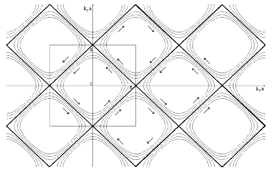
Figure 1: We show the lines of constant energy for the square lattice. The solid lines are the ones corresponding to zero energy. The arrows indicate the orbits in reciprocal space.

We would like at this point to describe a surprising behavior observed during the time evolution of wave packets. First, we note that their gaussian structure means that in reciprocal space we have a certain dispersion in k, which implies that several wave vectors will participate in the evolution of the wave function. This plays an important role as long as we are considering the wave vector associated with the velocity of the initial wave packet, lying along and around the lines of zero energy in the Brillouin zone of the square lattice. In Fig. 1 we show the lines of constant energy where the arrows signal the orbit in reciprocal space described by the wave vector.

As it is well described in the books of Solid Stateki , the quasimomentum satisfies an equation of motion analogous to the classical one; where one takes the group velocity $\textbf{v}=\frac{1}{\hbar}\frac{\partial\varepsilon}{\partial\textbf{k}}$ in the expression of the Lorentz force, which in turn determines that the wave vector moves along the lines of constant energy. First, consider k inside the region of energy zero, but close to its boundaries, it will describe a clockwise orbit in reciprocal space. As for k outside but close to the line, we get another trajectory described in counterclockwise sense. This will result in the appearance of vortices rotating in opposite directions when describing the evolution of the wave packet in direct space, where the ”orbits” are obtained after rotation by $\pi/2$.

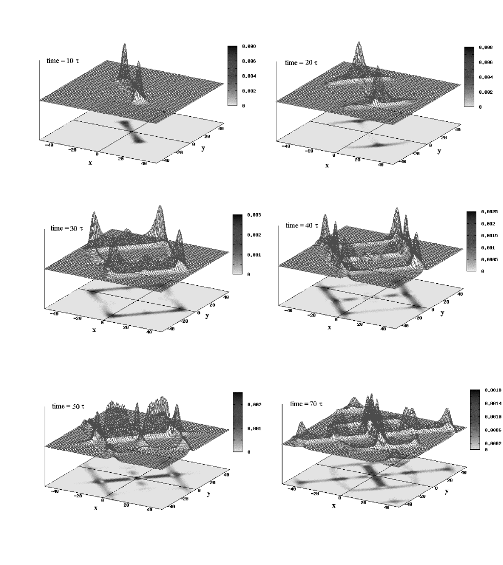
Figure 3: The same as Fig. 2 but for $\textbf{k}a=(\pi,0)$.

What is very interesting is to consider k on one of the lines of zero energy. In such a case due to the dispersion in k because of the gaussian structure of the initial packet, we discussed above, we have to take into account k values inside and outside the line, symmetrically distributed. Consequently, part of the wave (half of it) will describe a trajectory in the clockwise sense and the other half of the wave in the opposite sense, the resulting movements is similar to a swimmer doing breaststroke. As time goes, the wave packet starts moving in the direction of the velocity and then splits into two components that will join in a single component and so on. Consequently, two vortices with opposite angular velocities are formed. The wave remains stationary in a certain region of the lattice. See Fig. 2 where this remarkable effect is shown. Assuming now k with components ($\pi/a,0$), as shown in Fig. 1, four squares in reciprocal space participate in the movement of the packet reinforcing each other such that at a certain time the wave appears like is shown in Fig. 3. To get the evolution of the wave packet one has to follow the arrows in each of the four regions. Again, we observe the splitting and reconstruction of the wave, this time in several components. In this case, several vortices are present.

One encounters a similar effect when considering a 1-D crystal under the action of a dc electric field. When considering as an initial state a well localized state at a site in the system, the evolution of the packet is such that it is split into two symmetric parts, which oscillate with the Bloch frequency in opposite directionshn .

Let us assume k inside the region limited by the lines of zero energy but close to one of them. The wave function will split into two components in such a way that one part of the wave, the major part, will rotate clockwise while the rest will do counterclockwise. As for k outside the region but close to one of the lines, the reciprocal is true, the major part of the wave will perform a rotation counterclockwise. To illustrate this effect, consider now the wave vector of the initial wave packet, inside the region of the lines for $\epsilon=0$ but close to one of it, we took for example $\textbf{k}a=(1.4,1.4)$. As said above, the wave is split in two components, where the bigger part rotates clockwise and the smaller part rotates in the opposite sense. In this case this case it results in the appearance of two asymmetric vortices. See Fig. 4.

IV The effect of a dc electric field

We consider now the inclusion of a dc electric field in the equation of motion for the Wannier amplitudes. As a general trend we observe that the packet will propagate in a more complex way, but always in direction perpendicular to the electric field, as it was shown previouslyhp . This behavior is also present in the classical treatment of the problemla . From the view point of Quantum Mechanics, we understand this behavior since the electric field breaks the degeneracy of the on-site energies along the direction of the applied field, inhibiting hopping between these sites. First we take k on one of the lines of zero energy, for example ($\pi/2a,\pi/2a$) and the electric field along the diagonal, $\textbf{E}=(0.1,0.1)$, while the initial packet has $\sigma=1$. The wave is split while propagating but, due to the presence of the electric field, one part of the wave proceeds with a greater velocity, with a centroid trajectory similar to the one a snake performs when moving around. The other part that moves in opposite direction, remains close to the starting point. See Fig. 5 where we also show the centroid trajectory, and the MSD and participation as functions of time.

For the same configuration but for $\sigma=2$, we observe that the wave is not split and follows a trajectory quite similar to the classical one, i.e., the more so, the more extended is the initial wave packet, i.e., the greater is sigma. This comes about since a greater dispersion in direct space is related to a smaller one in reciprocal space. See Fig. 6. For the case $\sigma=3$ we confirm this behavior of the propagation of the wave. It is interesting to mention that the trajectories for $\sigma=2$ and $3$ are exactly the same. By increasing the intensity of the electric field we obtain a displacement of the centroid along a trajectory similar to the former one, the only difference is that in the case of stronger field the amplitude of the displacement as well as the period of the oscillations are reduced. This field effect is shown at the bottom left of Fig. 6.

A very peculiar effect is obtained by considering the electric field with components $(-0.1,0.1)$ and taken $\textbf{k}=(\pi/2a,\pi/2a)$. In this case we note that the ”swimmer” by doing breaststroke can displace itself along the perpendicular direction to the applied electric field. The vortices displacement is such that the centroid moves along a strait line, as shown in Fig.7. This should be compared with the case without electric field in which the packet remains stationary as shown in Fig. 2.

V Conclusions

We show in this work a novel effect of wave packet propagation in a two dimensional crystalline system under the action of combined magnetic and electric fields. Using the Runge Kutta method of forth order, we integrate the equations of motion in the Wannier representation, assuming as initial condition a gaussian wave packet with given velocity. We found the very interesting behavior of the wave function, namely, that by taking the initial velocity with the associated wave vector close to the lines of zero energy, the wave is split and reconstructed as time goes, with the appearance of a series of vortices. This effect comes about since we used a gaussian as an initial condition. This in turn, implies that one has to take into account a dispersion in the reciprocal space, so there are contributions of the lines of constant energy on both sides of the zero energy line, as explained above. Without the presence of the electric field, the wave remains in a definite region of the lattice. The inclusion of the electric field, produces a displacement of the vortices along the perpendicular direction of the applied field, showing a more complex behavior since now, besides the displacement, the wave is split and reconstructed as time goes. As for the centroid trajectory, for a configuration such that the applied electron field is parallel to the initial velocity, it describes a trajectory similar to the way a snake performs when moving around. In the classical treatment, the trajectory is a trochoid. For other configurations, i.e., for the wave packet with initial velocity perpendicular to the field, the centroid trajectory is a strait line. One last comment deserves to be made, the effects we described are the results of taking into account that the particle, besides being under the action of the fields, is subjected to a 2D crystal potential as well.

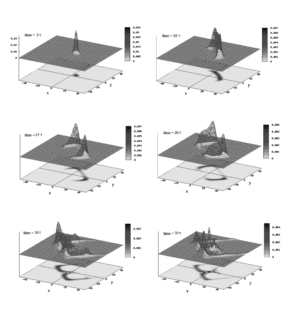
Figure 2: The time evolution of the wave packet for the following parameters: $\alpha=0.0242$, dispersion $\sigma=2$, and $\textbf{k}a=(\pi/2,\pi/2)$.

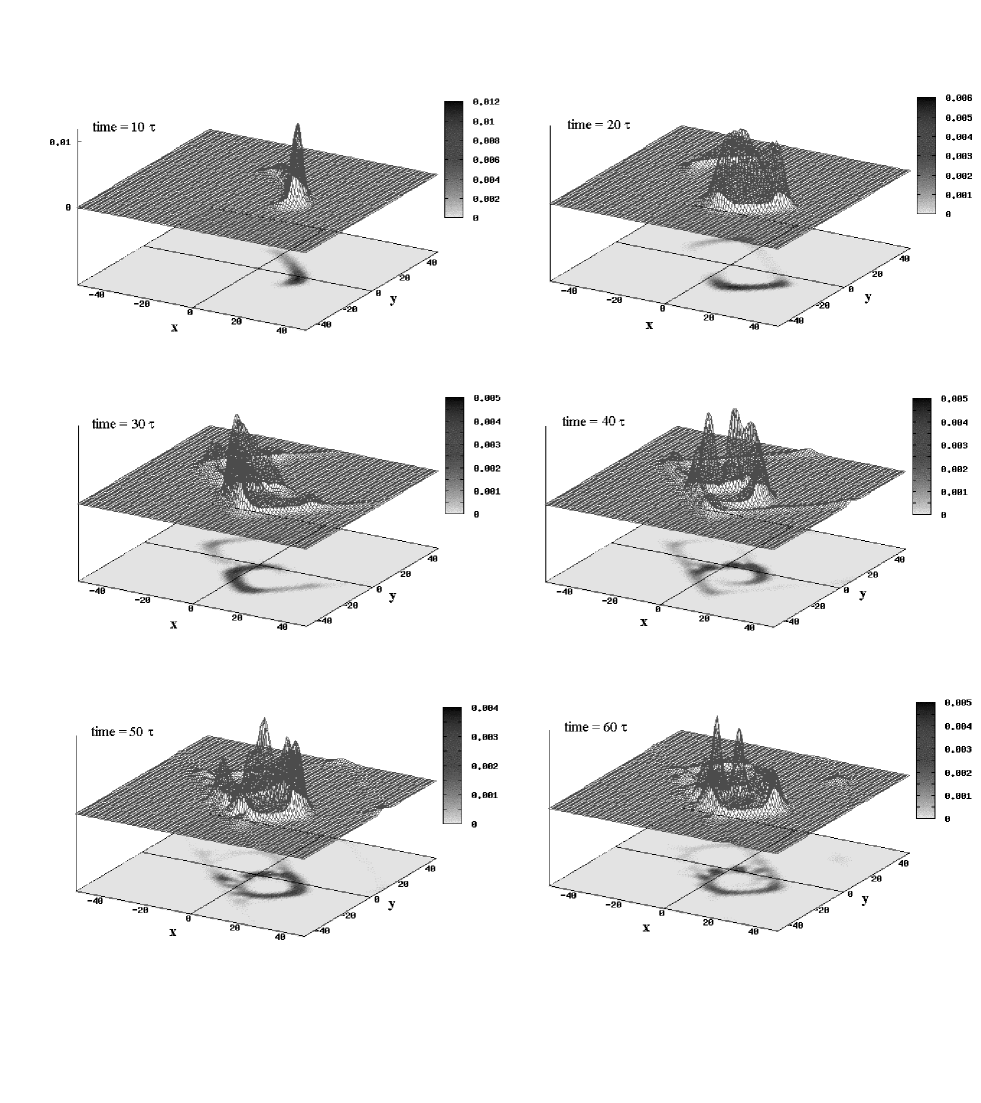
Figure 4: The same as Fig. 3 but for $\textbf{k}a=(1.4,1.4)$.

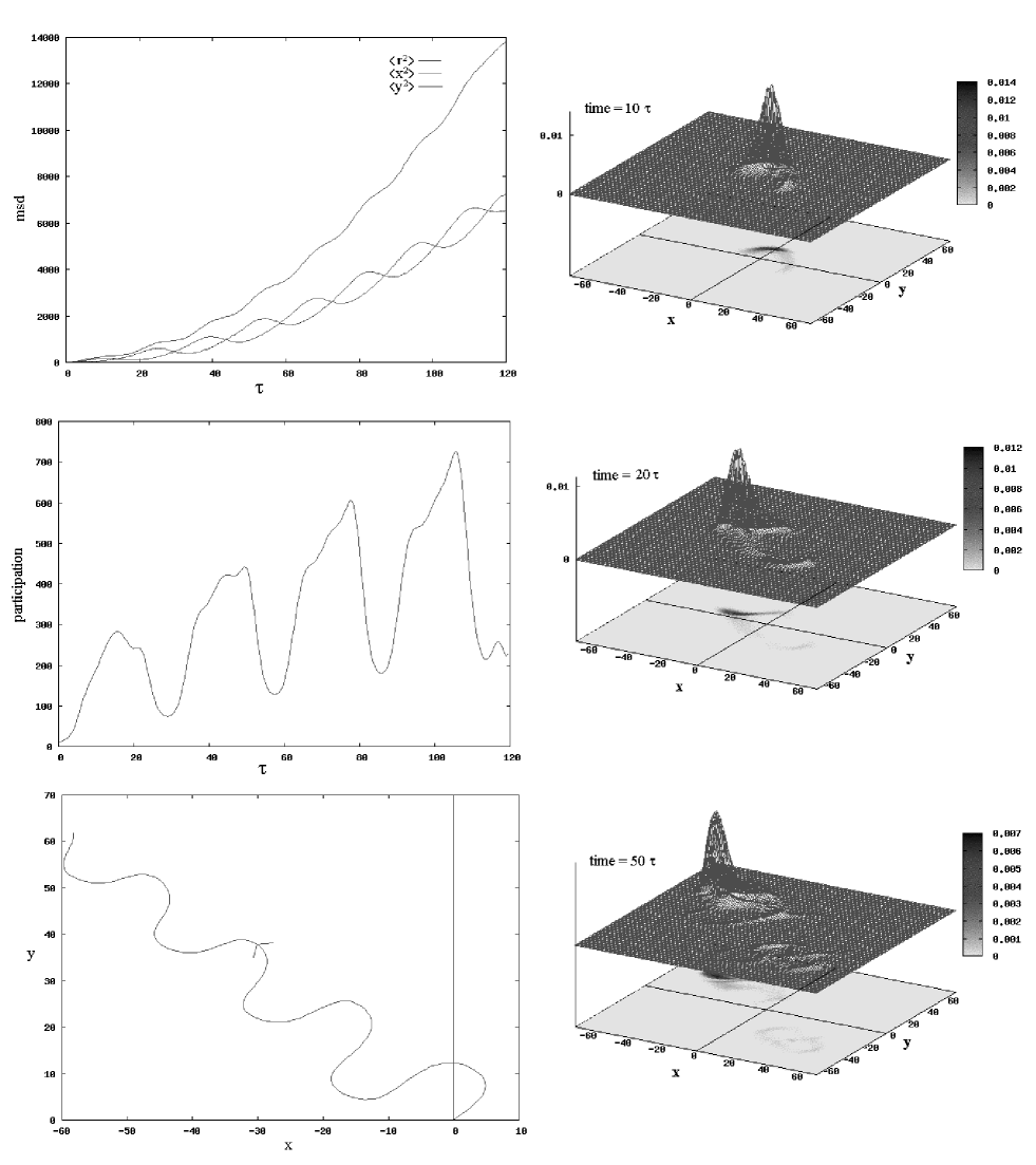
Figure 5: The time evolution of the wave packet for the following parameters: $\textbf{E}=(0.1,0.1)$, $\sigma=1$ and $\textbf{k}a=(\pi/2,\pi/2)$. On the left, MSD and participation as functions of time, and the centroid trajectory which resembles a trochoid.

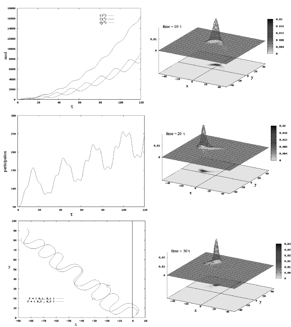
Figure 6: The same as Fig. 5 but for $\sigma=2$. The bottom left shows the trajectories of the centroids for two field intensities: $\textbf{E}=(0.1,0.1)$, and $\textbf{E}=(0.2,0.2)$. Note the different periods when varying the field intensity. See the text.

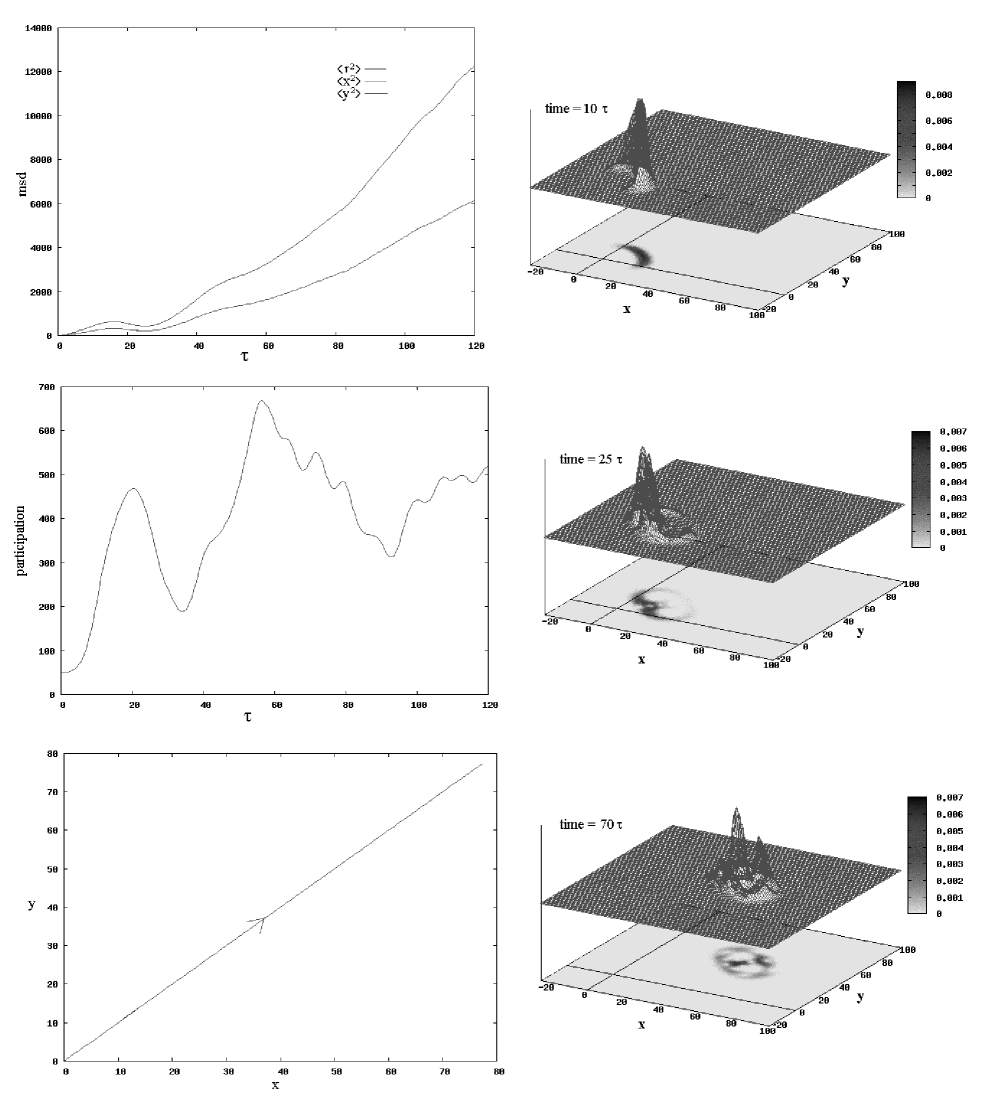
Figure 7: The same as Fig. 6 but for $\textbf{E}=(-0.1,0.1)$. Note the strait line described by the centroid.

References

- (1) F. Bloch, Z. Phys. 52, 555 (1928).
- (2) R. E. Peierls, Z. Phys. 80, 763 (1933).
- (3) L. Onsager, Philos. Mag. 43, 1006 (1952).
- (4) G. H. Wannier, Rev. Mod. Phys. 34, 1006 (1952).
- (5) J. Zak, Solid State Phys. 27, 1 (1972).
- (6) C. Albrecht, J. H. Smet, D. Weiss, K. von Klitzing, R. Hennig, M. Langenbuch, M. Suhrke, U. Rosler, V. Umansky, and H. Schweizer, Phys. Rev. Lett. 83, 2234 (1999).
- (7) R. Ketzmerick, K. Kruse, D. Springsguth, and T. Geisel, Phys. Rev. Lett. 84, 2929 (2000).
- (8) I. V. Krasovsky, Phys. Rev. Lett. 85, 4920 (2000).
- (9) A. Kunold and M. Torres, Phys. Rev. B 61, 9879 (2000).
- (10) H. N. Nazareno and P. E. de Brito, Phys. Rev. B 64, 45112 (2001).
- (11) Enrique Munoz, Zdenka Barticevic and Monica Pacheco, Phys. Rev. B 71, 165301 (2005).
- (12) D. R. Hofstadter, Phys. Rev. 14, 2239 (1976).
- (13) C. Albrecht, J. H. Smet, K. von Klitzing, D. Weiss, V. Umansky and H. Schweizer, Phys. Rev. Lett. 86, 147 (2001).
- (14) F. Wegner, Z. Phys. B: Condens. Matter, 36, 209 (1980).
- (15) P. W. Anderson, Phys. Rev. 109, 1492 (1958).
- (16) C. Kittel, Quantum theory of solids, John Wiley & Sons, 2nd. Ed. (1987).
- (17) H. N. Nazareno and J. C. Gallardo, Phys. Stat. Solid (b) 153, 179 (1989).
- (18) L. Landau and E. Lifchitz, The Classical Theory of Fields, Pergamon Press 4th Ed. (1987).