Mumford dendrograms

Abstract.

An effective $p$-adic encoding of dendrograms is presented through an explicit embedding into the Bruhat-Tits tree for a $p$-adic number field. This field depends on the number of children of a vertex and is a finite extension of the field of $p$-adic numbers. It is shown that fixing $p$-adic representatives of the residue field allows a natural way of encoding strings by identifying a given alphabet with such representatives. A simple $p$-adic hierarchic classification algorithm is derived for $p$-adic numbers, and is applied to strings over finite alphabets. Examples of DNA coding are presented and discussed. Finally, new geometric and combinatorial invariants of time series of $p$-adic dendrograms are developped.

1. Introduction

A dendrogram is often the output of a hierarchical classification algorithm. In the usual agglomerative methods, it is obtained from data by a distance function which is adjusted after each iteration to the clusters obtained in the previous step. Classically, the distance is euclidean, and the hierarchical structure is fitted to the data. The analyst then has to decide by other means whether the resulting dendorgram represents the underlying hierarchical structure of the data, or not. In the $p$-adic world, however, there is no ambiguity concerning the interpretation of dendrograms. The reason is that the $p$-adic distance is ultrametric. This has the effect that a $p$-adic dendrogram correctly represents the hierarchies within a given set of $p$-adic numebrs, of course with respect to the $p$-adic metric. Another effect is, as we will show, that $p$-adic classification is algorithmically much simpler than its classical counterpart. The consequence for data mining lies in the shift from classification to data encoding.

If the dendrogram $X$ is known, then its $p$-adic encoding can be effected by associating paths from the top cluster down to the data with $p$-adic numebrs. This is in fact an embedding of $X$ into the $p$-adic Bruhat-Tits tree which can be seen as a “universal dendorgram”. This embedding will be made precise in this article. Strings over an alphabet are the only instance known to the author, in which $p$-adic data encoding can be realised in a straightforward manner. The encoding depends on the coefficients in $p$-adic expansions associated to the alphabet. Examples of $p$-adic DNA encoding are proposed and discussed.

Time series of $p$-adic dendrograms give rise to new geometric invariants. namely, if translations along geodesic lines in the Bruhat-Tits tree can be identified, a discrete group action can be estimated in important cases. This action then leads to a dynamic system on a so-called Mumford curve, the $p$-adic analogon of a riemann surface. Studying this dynamic system will yield pararmeters whic can be used e.g. for extrapolating hierarchical data in time.

Possible applications of $p$-adic dendrograms are coding theory of graphs and strings. Another area of application can be spatial reasoning and querying, including space-time issues. The time series point of view is naturally applicable to strings. The idea of studying $p$-adic dendrograms is taken from [8]. Linear fractions are considered in [5] in the $p$-adic and real case simultaneously. A description for a general audience of the $p$-adic Bruhat-Tits tree and some of its discrete symmetries can be found in [3].

2. Embedding a dendrogram into the $p$-adic Bruhat-Tits tree

In order to embed a dendrogram $X$ into the $p$-adic Bruhat-Tits tree, we first define $X$ as the dendrogram for its data plus an extra point $\infty$. The reason is that in this way the top cluster becomes the vertex uniquely determined by $\infty$ and two data points at maximal distance. This viewpoint leads to the term projective dendrogram, and we will see that in the $p$-adic case, it is associated to the $p$-adic projective line minus the $p$-adic numbers representing the data and $\infty$.

2.1. Abstract dendrograms

Dendrograms represent hierarchies within data, and are therefore trees, i.e. graphs without loops. Subsets of data points are clusters represented by the vertices, and inclusions of clusters are represented by paths between the corresponding vertices. It is useful to distinguish between clusters and data in the same way as one distinguishes sets from their elements: even if certain clusters are singletons, they are nevertheless not data in the same way as the set ${\left\{x\right\}}$ is in a strict sense not the same thing as the point $x$. Hence, in our viewpoint, the data will not be part of, but at the boundary of a dendrogram. Hence, we will allow graphs to have unbounded edges.

Definition 2.1.

A graph is a quadruple $\Gamma=(\Gamma^{0},\Gamma^{\prime},\partial,\iota)$, where $\Gamma^{0}$ and $\Gamma^{\prime}$ are sets, $\partial\colon\Gamma^{\prime}\to\Gamma^{0}$ is a map, and $\iota\colon\Gamma^{\prime}\to\Gamma^{\prime}$ is an idempotent map (i.e. $\iota\circ\iota={\rm id}$). The elements of $\Gamma^{0}$ are called vertices, and those of $\Gamma^{\prime}$ flags. $\partial$ is called the boundary map, and $\iota$ the inversion. A graph $\Gamma$ is finite if $\Gamma^{0}$ and $\Gamma^{\prime}$ are both finite.

The inversion yields an equivalence relation on the set of flags: $F_{1}\sim F_{2}$ iff $F_{1}=F_{2}$ or $F_{1}=j(F_{2})$. The equivalence classes under $\sim$ are called the edges of $\Gamma$. The set of edges is denoted by $\Gamma^{1}=\Gamma^{\prime}/\sim$. An edge is called unbounded if it consists of a single flag, otherwise it is called internal. We denote the set of internal resp. unbounded edges by $\Gamma^{1}_{0}$ resp. $\Gamma^{1}_{\infty}$.

A graph $\Gamma$ has a topological model $\lvert\Gamma\rvert$, obtained by identifying each flag $F$ with the half-open interval $[0,1)_{F}$ and pasting $\partial F$ to $F$, and then taking the quotient by $\sim$. This model reflects important topological properties of the graph, such as the number of connected components or the number of “holes”, i.e. minimal loops in $\Gamma$. These quantities are known as the Betti numbers $h_{0}(\lvert\Gamma\rvert,\mathbb{R})$ and $h_{1}(\lvert\Gamma\rvert,\mathbb{R})$ from algebraic topology, where they are introduced as the dimension of certain real vector spaces. For finite graphs, there is an important formula which relates the Betti numbers to the combinatorial data:

$$h_{0}(\lvert\Gamma\rvert,\mathbb{R})-h_{1}(\lvert\Gamma\rvert,\mathbb{R})=\#\Gamma^{0}-\#\Gamma^{1}_{0},$$

known as the Euler formula.

A graph $\Gamma$ is a tree if it is connected and without loops, or, equivalently, if the Betti numbers of $\lvert\Gamma\rvert$ satisfy $h_{0}(\lvert\Gamma\rvert,\mathbb{R})=1$ and $h_{1}(\lvert\Gamma\rvert,\mathbb{R})=0$.

A rooted tree is a pair $(T,v)$, where $T$ is a tree and $v\in T^{0}$ is a vertex. The distinguished vertex $v$ is called the root and makes a rooted tree $(T,v)$ into a directed tree by orienting all edges away from $v$, i.e. an internal edge $e$ with boundary ${\left\{w_{1},w_{2}\right\}}$ is oriented from $w_{1}$ to $w_{2}$, if $w_{1}$ is closer to $v$ than $w_{2}$ is, and an unbounded edge $e^{\prime}$ is oriented away from the unique vertex $\partial{e^{\prime}}$.

By an abstract dendrogram we mean a finite rooted tree $\mathcal{T}=(T,v)$, all of whose vertices originate in at least two edges (unbounded or not). It is labelled, if its unbounded edges are labelled by some bijective map $\lambda\colon T^{1}_{\infty}\to L$, where $L$ is a set whose elements are called labels. A projective dendrogram is a labelled abstract dendrogram $\mathcal{T}$ whose root originates in an umbounded edge labelled $\infty$ and at least two more edges. The unbounded edges not labelled $\infty$ are called the datapoints or data underlying $\mathcal{T}$, and will be denoted by $D$. Figure 1 illustrates a projective dendrogram with three data points. The reason for calling it “projective” will become apparent in later subsections.

Figure 1. Projective dendrogram with three datapoints.

Remark 2.2.

To call unbounded edges of a dendrogram $\mathcal{T}$ “data” seems to be in contradiction to the initial purpose of having data not be part of a dendrogram. However, by looking at the topological model, we see first that an unbounded edge is nothing but a half-line in the tree $T$ underlying $\mathcal{T}$. The ends of $T$ are equivalence classes of halflines, where halflines differring only in finitely many internal edges are equivalent. According to graph theory, the ends form the boundary $\partial T$ of $T$. Hence, we have in fact identified $\partial T\cong T^{1}_{\infty}$ with data and $\infty$.

Given some projective dendrogram $\mathcal{T}=(T,v,\lambda,D)$, there is an order relation $<$ on $T^{1}\setminus\lambda^{-1}(\infty)$: $e<e^{\prime}$, if $e$ lies on the path from $\infty$ to $e^{\prime}$. If $e$ and $e^{\prime}$ originate in some vertex $v$, impose any total order $<_{v}$ on the edges originating in $v$ in order to break ties. This extends to a total order on data as follows: the lexicographic order with respect to $<$ and all $<_{v}$ on the reduced words $\infty\cdots e$ associated to minimal paths $w_{e}$ (i.e. paths without backtracking) from $\infty$ to $e$ induces a total order on $D$ via the unique bijection between $D$ and ${\left\{w_{e}\mid e\in T^{1}_{\infty}\right\}}$ induced by $\lambda$. A projective dendrogram together with a total ordering $<$ on its data is called ordered. We call a minimal path in a tree geodesic.

A metric on a projective dendrogram is a function $\mu\colon T^{1}_{0}\to\mathbb{N}\setminus{\left\{0\right\}}$, and defines in an obvious manner a distance $d\colon T^{0}\times T^{0}\to\mathbb{N}$. This induces a level structure $\ell\colon T^{0}\to\mathbb{N},\;w\mapsto\ell(w)=d(v,w)$, where $v$ is the root. Figure 2 displays a projective dendrogram with level structure and $\infty$ on top.

2.2. The binary case

Let $X=(T,v,D,<,\mu)$ be an ordered projective dendrogram with metric. In this subsection, we assume that $T$ is a binary tree, i.e. each vertex $w\in T^{0}$ has precisely two (internal or unbounded) directed outoing edges $e_{0}(w)<e_{1}(w)$. With $e_{0}:=e_{0}(v)$ and $e_{1}:=e_{1}(v)$ we have that $T\setminus{\left\{v\right\}}$ is the disjoint union of the two branches $\Gamma_{0}\ni e_{0}$ and $\Gamma_{1}\ni e_{1}$. $\Gamma_{0}$ and $\Gamma_{1}$ are themselves projective dendrograms, if the $e_{i}$ are labelled $\infty_{i}$. We define functions

$$\chi_{0}\colon\Gamma_{0}^{1}\to{\left\{0,1\right\}},\; e\mapsto\begin{cases}0,&\exists w\in T^{0}\colon e=e_{0}(w)\\ 1,&\text{otherwise}\end{cases}$$

$$\chi_{1}\colon\Gamma_{1}^{1}\to{\left\{0,1\right\}},\; e\mapsto\begin{cases}0,&\exists w\in\Gamma_{1}^{0}\colon e=e_{1}(v)\\ 1,&\text{otherwise}\end{cases}$$

Together, $\chi_{0}$ and $\chi_{1}$ define a function $\chi\colon T^{1}\to{\left\{0,1\right\}}$ such that $\chi(e_{0})=0$ and $\chi(e_{1})=1$. This extends to a function on the set $\mathcal{G}(\infty,D)$ of directed geodesics $\gamma_{x}$ from $\infty$ to any datum $x\in D$

$$\chi\colon\mathcal{G}(\infty,D)\to\mathbb{Q}_{2},\;\gamma_{x}\mapsto\sum\limits_{e\in\gamma_{x}}\chi(e)2^{\ell(o(e))},$$

where $o(e)$ denotes the origin vertex of the edge $e$, and $\ell$ is the level function on $X$. Together with the identification $\mathcal{G}(\infty,D)\cong D$, we obtain the $2$-adic encoding $\chi\colon D\to\mathbb{Q}_{2}$ of binary data.

Remark 2.3.

The coding function $\chi$ is in fact $\mathbb{Z}_{2}$-valued. Even more, its values are natural numbers, because $X$ is finite. By construction, the values $0$ and $1$ are taken by $\chi$ for any projective dendrogram. In fact, $\chi(x_{0})=0$ and $\chi(x_{n})=1$, if $D={\left\{x_{0}<\dots<x_{n}\right\}}$.

Example 2.4.

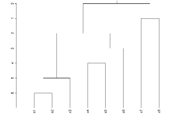
Figure 2. A projective dendrogram with level structure.

The dendrogram in Figure 2 has the $2$-adic encoding $\chi$ given by:

$$\begin{array}[]{llll}x_{1}=0,&x_{2}=2^{6},&x_{3}=2^{5},&x_{4}=2^{2}\\ x_{5}=2^{2}+2^{4},&x_{6}=2^{2}+2^{3},&x_{7}=2^{0}+2^{1},&x_{8}=1.\end{array}$$

This encoding differs slightly from the $2$-adic encoding of the same dendrogram in [9].

2.3. The Bruhat-Tits tree for $p$-adic fields

It was observed that an encoding of dendrograms with $p$-adic numbers from $\mathbb{Q}_{p}$ leads to considering subtrees of the Bruhat-Tits tree $\mathscr{T}_{\mathbb{Q}_{p}}$ [1, 2]. Here, we intend to prepare an effective embedding of dendrograms into the Bruhat-Tits tree, which is going to be made precise in Section 2.4. The preparation consists in reviewing the construction of $\mathscr{T}_{\mathbb{Q}_{p}}$ and the variants for finite extension fields $K$ of $\mathbb{Q}_{p}$, as the latter turns out too small in general for encoding data.

2.3.1. The Bruhat-Tits tree for $\mathbb{Q}_{p}$

The $p$-adic field $\mathbb{Q}_{p}$ can be defined as the field of Laurent series

$$\sum\limits_{\nu=-m}^{\infty}a_{\nu}p^{\nu},\quad a_{\nu}\in{\left\{0,\dots,p-1\right\}}.$$

It is well known that the $p$-adic norm induces a topology on the field $\mathbb{Q}_{p}$ which makes it into a totally disconnected space. This is, however, compensated by the fact that $p$-adic discs never overlap. Hence, the ultrametric inequality provides us with a tree-like topology on the set of discs. It is precisely this hierarchical structure of discs which makes $p$-adic numbers interesting for hierarchical classification. Consider the unit disc

$$\mathbb{D}={\left\{x\in\mathbb{Q}_{p}\colon\lvert x\rvert_{p}\leq 1\right\}}=B_{1}(0).$$

It is a subring of $\mathbb{Q}_{p}$ which coincides with the ring of $p$-adic integers

$$\mathbb{Z}_{p}={\left\{\sum\limits_{\nu=0}^{\infty}a_{\nu}p^{\nu}\colon a_{\nu}\in{\left\{0,\dots,p-1\right\}}\right\}}.$$

It has a unique maximal ideal $p\mathbb{Z}_{p}$, and this ideal coincides with the maximal “open” (non-trivial) subdisc ${\left\{x\in\mathbb{Q}_{p}\mid\lvert x\rvert_{p}<1\right\}}$. It is a standard fact from algebra that the quotient of a unital commutative ring by a maximal ideal is a field. In our case, $\mathbb{Z}_{p}/p\mathbb{Z}_{p}\cong\mathbb{F}_{p}$, the finite field with $p$ elements. This is well known and follows from the fact that the unit disc is covered by the finite number of translates of the subdisc $p\mathbb{Z}_{p}$:

$$\mathbb{Z}_{p}=\bigcup_{x=0}^{p-1}(x+p\mathbb{Z}_{p}),$$

which says in a fancy way that there are precisely $p$ choices for the constant term in the power series expansion of any $p$-adic integer. Hence, we have a hierarchical structure of a disc with $p$ maximally smaller subdiscs. By rescaling and translation, it follows immediately that any $p$-adic disc has precisely $p$ smaller subdiscs which are maximal as subdiscs. Observe that $p\mathbb{Z}$ has precisely one minimal bigger disc containing $p\mathbb{Z}_{p}$, namely $\mathbb{D}$. Again, this holds for all $p$-adic discs. The consequence is that the set of all subdiscs of $\mathbb{Q}_{p}$ form a $p+1$-regular tree $\mathscr{T}_{\mathbb{Q}_{p}}$, called the Bruhat-Tits tree for $\mathbb{Q}_{p}$. Figure 3 shows an illustration of $\mathscr{T}_{\mathbb{Q}_{2}}$ taken from [3, Fig. 5].

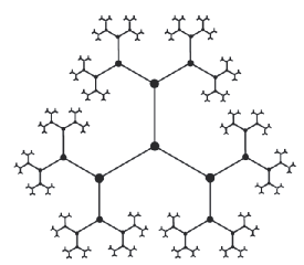
Figure 3. The Bruhat-Tits tree for $\mathbb{Q}_{2}$.

2.3.2. Bruhat-Tits trees for $p$-adic number fields

The field $\mathbb{R}$ of real numbers is complete with respect to the archimedean distance $\lvert\cdot\rvert_{\mathbb{R}}$. In the same way is the field $\mathbb{Q}_{p}$ complete with respect to $\lvert\cdot\rvert_{p}$. However, neither $\mathbb{R}$ nor $\mathbb{Q}_{p}$ is algebraically closed. In the archimedean case, the algebraic closure of $\mathbb{R}$ is the field $\mathbb{C}$ of complex numbers, and $\mathbb{C}$ is a two-dimensional vector space over the scalar field $\mathbb{R}$. By definition, the degree of a field extension $L$ over $K$ (meaning $K$ is a subfield of a field $L$) is the dimension of $L$ as a vector space over the scalar field $K$. If that degree is finite, then $L$ is called a finite extension of $K$. Hence, the degree of $\mathbb{C}$ over $\mathbb{R}$ is $2$, and $\mathbb{R}$ has no other finite field extensions. In contrast, $\mathbb{Q}_{p}$ has extension fields of arbitrary degree. Hence, the algebraic closure of $\mathbb{Q}_{p}$ is an infinite extension of $\mathbb{Q}_{p}$. Assume that a finite extension field $K$ of $\mathbb{Q}_{p}$ of degree $n$ be given. Then it is known that the distance $\lvert\cdot\rvert_{p}$ extends uniquely to a norm $\lvert\cdot\rvert_{K}$ on $K$, and $K$ is complete with respect to $\lvert\cdot\rvert_{K}$ [6, §5.3]. Again the unit disc

$$\mathcal{O}_{K}={\left\{x\in K\colon\lvert x\rvert_{K}\leq 1\right\}}$$

is a ring with unique maximal ideal

$$\mathfrak{m}_{K}={\left\{x\in K\colon\lvert x\rvert_{K}<1\right\}},$$

and $\kappa=\mathcal{O}_{K}/\mathfrak{m}_{K}$ is a finite field extension of $\mathbb{F}_{p}$, called the residue field. It is finite with $p^{f}$ elements, if $f$ is the degree of $\kappa$ over $\mathbb{F}_{p}$. In general, the degree $n$ is not smaller than $f$, but if $n=f$, then $K$ is called unramified over the subfield $\mathbb{Q}_{p}$. A finite extension field of $\mathbb{Q}_{p}$ is also called a $p$-adic number field, and the elements of $\mathbb{Q}_{p}$ are sometimes called rational $p$-adic numbers.

In any case, if $K$ is a $p$-adic number field with $\kappa\cong\mathbb{F}_{p^{f}}$, then in the same manner as with $\mathbb{Q}_{p}$ the unit disc $\mathcal{O}_{K}$ is covered by $p^{f}$ translates of the subdisc $\mathfrak{m}_{K}$. This gives rise to the Bruhat-Tits tree $\mathscr{T}_{K}$ for $K$ which is an infinite $p^{f}+1$-regular tree. In other words, the number of edges emanating from a vertex of $\mathscr{T}_{K}$ depends on the residue field $\kappa$ which can be the same for different extension fields of $\mathbb{Q}_{p}$. So, the choice of unramified extensions is in some sense optimal for constructing the Bruhat-Tits trees.

In general, $p$ will not be a prime element of $\mathcal{O}_{K}$, but this is true in the unramified case. In fact, for $K$ unramified of degree $f$ over $\mathbb{Q}_{p}$, it holds true that $\mathfrak{m}_{K}=p\mathcal{O}_{K}$, and every element of $\mathcal{O}_{K}$ has an expansion

$$x=\sum\limits_{\nu=0}^{\infty}a_{\nu}p^{\nu},\quad a_{\nu}\in\mathfrak{R},$$

where $\mathfrak{R}$ is a system of $p^{f}$ representatives modulo $p\mathcal{O}_{K}$. However, in the ramified case, $p$ is not a prime in $\mathcal{O}_{K}$. But also in this case, the maximal ideal $\mathfrak{m}_{K}$ is of the form $\pi\mathcal{O}_{K}$ for some prime $\pi\in\mathcal{O}_{K}$. It is always possible to choose $\pi$ such that $\lvert\pi\rvert_{K}=p^{-1/e}$ for some natural number $e\geq 1$ [6, §5.4]. This number $e$ is called the ramification index of $K$ over $\mathbb{Q}_{p}$, and $K$ is ramifed over $\mathbb{Q}_{p}$, if $e>1$. The extension $K$ over $\mathbb{Q}_{p}$ is called purely ramified, if $f=1$.

2.3.3. Cyclotomic $p$-adic fields

It is known that $\mathbb{Q}_{p}$ contains the $p-1$-st of unity, but not the $p^{f}-1$-st roots of $1$ for $f>1$. Therefore, we discuss the fields $\mathbb{Q}_{p}(\zeta)$ obtained by adjoining to $\mathbb{Q}_{p}$ the $n$-th roots of unity which are all powers of $\zeta$, a primitive $n$-th root of $1$. We will first consider the case that $p$ is prime to $n$. In that case, $\mathbb{Q}_{p}(\zeta)$ is unramified over $\mathbb{Q}_{p}$, the degree is the smallest number $f$ such that $p^{f}\equiv 1\mod n$, and ${\left\{1,\zeta,\dots,\zeta^{f-1}\right\}}$ represents an $\mathbb{F}_{p}$-basis of $\kappa=\mathbb{F}_{p^{f}}$ in $\mathcal{O}_{\mathbb{Q}(\zeta)}$ which equals the polynomial ring $\mathbb{Z}_{p}[\zeta]$ [11, II.(7.12)]. That means, we can choose

$$\mathfrak{R}={\left\{\sum\limits_{\nu=0}^{f-1}a_{\nu}\zeta^{\nu}\colon a_{\nu}\in{\left\{0,\dots,p-1\right\}}\right\}}$$

as a system of representatives which is in bijection with a subset of $\mathbb{N}^{f}$.

The most economic choice for $n$ is certainly $p^{f}-1$. In that case, $\mathbb{Q}(\zeta)$ is again unramified of degree $f$ over $\mathbb{Q}_{p}$, and

$$\mathfrak{R}_{T}={\left\{0,1,\zeta,\dots,\zeta^{p^{f}-2}\right\}}$$

is an alternative set of representatives for $\kappa=\mathbb{F}_{p^{f}}$. This is a consequence of Hensel’s Lemma [6, Thm. 5.4.8] (cf. [6, §5.4]. The elements of $\mathfrak{R}_{T}$ are called the Teichmüller representatives of $\mathbb{F}_{p^{f}}$ and have the characterising property that the residue class of $\zeta$ generates the multiplicative group $\mathbb{F}_{p^{f}}^{\times}=\mathbb{F}_{p^{f}}\setminus{\left\{0\right\}}$. For example, if $f=1$, then already $\mathbb{Q}_{p}$ contains the $p-1$-st roots of $1$ which form the Teichmüller representatives in that case [6, Cor. 4.3.8].

Another important case is when $\zeta$ is a primitive $p^{m}$-th root of unity. Then $\mathbb{Q}_{p}(\zeta)$ is purely ramified over $\mathbb{Q}_{p}$ of degree $e=(p-1)p^{m-1}$ [11, II.(7.13)].

2.4. Algebraic $p$-adic dendrograms

The reason for introducing the Bruhat-Tits tree $\mathscr{T}_{K}$ also for finite extensions $K$ of $\mathbb{Q}_{p}$ is that the number of children of a vertex can in principle be unbounded. This means that $K$ must be taken sufficiently large in order for a dendrogram to be embeddabe into $\mathscr{T}_{K}$. In this subsection, we will effect the embedding, define $p$-adic dendrograms and discuss these from a geometric perspective.

2.4.1. Cyclotomic encoding

Let $X=(T,v,D,\mu)$ be a projective dendrogram. By the children ${\rm ch}(v)$ of a vertex $w\in T^{0}$ we mean the outgoing edges of $v$ in $T^{1}$ which are not labelled $\infty$. Let

$$m=\max{\left\{\#{\rm ch}(w)\mid w\in T^{0}\right\}},$$

and $f$ minimal such that $m\leq p^{f}$. $K=\mathbb{Q}_{p}(\zeta)$ will denote the cyclotomic field with $\zeta$ a primitive $p^{f}$-th root of unity, and assume that $\mathfrak{R}$ is a full system of representatives modulo $p\mathcal{O}_{K}$ containing $0$ and $1$. Generalising the binary case, $\chi_{w}\colon{\rm ch}(w)\to\mathfrak{R}$ is now an inclusion map for every vertex $w\in T^{0}$ such that $0\in{\rm im}\chi_{w}$, and $1\in{\rm im}\chi_{v}$. These maps form together a map $\chi\colon T^{1}\to\mathfrak{R}$ which yields a $p$-adic encoding map

$$\mathcal{G}(\infty,D)\to K,\;\gamma_{x}\mapsto\sum\limits_{\gamma_{x}}\chi(e)p^{\ell(o(e))},$$

where $\ell\colon T^{0}\to\mathbb{N}$ is the level map derived from the metric $\mu$ as in Section 2.1. Again, as in the binary case, the natural identification $D\cong\mathcal{G}(\infty,D)$ yields a $p$-adic encoding $\chi\colon D\to K$ of the data. In the case $m=2$, we recover the binary encoding as in Section 2.2 for ordererd dendrograms, if the local encoding maps $\chi_{w}\colon{\rm ch}(w)\to\mathfrak{R}={\left\{0,1\right\}}$ are chosen appropriately.

Remark 2.5.

If a dendrogram is binary, or the prime $p$ is sufficiently large (not smaller than the largest number of children of any given vertex), then a rational $p$-adic encoding is possible. In this case, data will be represented by finite $p$-adic expansions, hence by natural numbers. Restricting to rational $p$-adic encoding has the disadvantage that $p$ is a fixed bound for the number of possible children vertices in dendrograms. Hence, if there is no a priori bound in data, then it is necessary to allow unramified extensions of $\mathbb{Q}_{p}$ of arbitrary degree. From a computational point of view it is probably most interesting to keep the prime $p$ as low as possible, i.e. $p=2$.

2.4.2. Dendrograms and the $p$-adic projective line

Let $X$ be a projective dendrogram. In Section 2.4.1, we have constructed an embedding of the underlying data $D\to K$ into a $p$-adic number field $K$. From a geometric viewpoint, this is an embedding of $D$ into the $p$-adic affine line. It is often convenient to treat points on the affine line and $\infty$ on an equal footing. The geometric space enabling this is the projective line. Hence, we consider a $p$-adic number from $K$ as a point in the $p$-adic projective line $\mathbb{P}^{1}$. The space $\mathbb{P}^{1}$ is a $p$-adic manifold defined over $\mathbb{Q}_{p}$ and whose $K$-rational points are given by $\mathbb{P}^{1}(K)=K\cup{\left\{\infty\right\}}$ for any field $K$ containing $\mathbb{Q}_{p}$. Here, we consider only the case that $K$ is a $p$-adic number field.

In Section 2.3, we have constructed for each $K$ the Bruhat-Tits tree $\mathscr{T}_{K}$ by associating to each disc in $K$ a vertex of $\mathscr{T}_{K}$. To an inclusion $B\subseteq B^{\prime}$ of disks corresponds a geodesic path between the associated vertices $w$ and $w^{\prime}$. It is a fact that any strictly descending infinite chain of discs in $K$

(1) $$B_{1}\supseteq B_{2}\supseteq\dots$$

converges to a $K$-rational point: ${\left\{x\right\}}=\bigcap B_{\nu}$ with $x\in\mathbb{P}^{1}(K)$. In the tree $\mathscr{T}_{K}$, the chain (1) corresponds to an infinite geodesic half-line

and the $p$-adic number $x$ lies at its end. It is a well known fact that the ends of $\mathscr{T}_{K}$ correspond bijectively to $\mathbb{P}^{1}(K)$. Now let $S\subseteq\mathbb{P}^{1}(K)$ be a finite set of $p$-adic numbers. Then we can form the $*$-tree which is the smallest subtree $T^{*}\langle S\rangle$ of $\mathscr{T}_{K}$ whose ends correspond to $S$. If $S\setminus{\left\{\infty\right\}}\subseteq\mathscr{O}_{K}$ and $S$ contains $0$ and $1$, then $T^{*}\langle S\rangle$ can be made in a natural way to a projective dendrogram. First observe that three disctinct points $x,y,z\in\mathbb{P}^{1}(K)$ define a unique vertex $v(x,y,z)$ in $\mathscr{T}_{K}$: it is the intersection of the three geodesics ending in ${\left\{x,y,z\right\}}$. Hence, $T^{*}\langle S\rangle$ contains the vertex $v=v(0,1,\infty)$ corresponding to the unit disc $\mathcal{O}_{K}$. Choose $v$ as the root. As $S\subseteq\mathcal{O}_{K}\cup{\left\{\infty\right\}}$, all vertices on the half-line $]v,\infty[$ have precisely two emanating edges in $T^{*}\langle S\rangle$. By defining $T^{0}_{S}$ to be the set of vertices $w$ in $T^{*}\langle S\rangle$ with $\#{\rm ch}(w)\geq 2$, and $T^{1}_{S}$ the set of geodesic paths $]w,w^{\prime}[$ between $w\in T^{0}_{S}$ and $w^{\prime}\in T^{0}_{S}\cup S$ not containing a vertex from $T^{0}_{S}$, we obtain a tree $T_{S}$ whose data $D_{S}$ are the half-lines $]w,s[$ with $w\in T^{0}_{S}$, $w\in S\setminus{\left\{\infty\right\}}$ and not containing any vertex from $T^{0}_{S}$. This yields a projective dendrogram $X_{S}=(T_{S},v,D_{S},\mu_{S})$, where the metric $\mu$ is defined as the number $\mu(e)$ of edges in $\mathscr{T}_{K}$ on the geodesic path corresponding to $e\in T^{1}_{S}$. It is clear that there is a natural $p$-adic encoding $\chi_{S}\colon D_{S}\to S$ with numbers from $K$.

A tree in which every vertex $v$ has more than two emanating edges is called stable. This is, in a way, a kind of minimal representation of a tree. In that sense, $T_{S}$ is the stabilisation of $T^{*}\langle S\rangle$. It is clear that for any projective dendrogram $X=(T,v,D,\mu)$ a $p$-adic endoding $\chi\colon D\to K$ as in Section 2.4.1 yields a tree $T^{*}\langle\chi(D)\rangle$ whose stabilisation is tree-isomorphic to $T$. Hence, a $p$-adic encoding $\chi$ means in $p$-adic geometry an embedding of projective dendrograms into $\mathscr{T}_{K}$ for some $p$-adic field $K$ through the assignment

$$\Xi\colon X\mapsto\mathbb{P}^{1}\setminus(\chi(D)\cup{\left\{\infty\right\}}).$$

This assignment is a map from the space $\mathfrak{D}_{n}$ of dendrograms on $n$ data to the space $\mathfrak{M}_{0,n+1}$ of $n+1$-pointed projective lines. Any pointed projective line is, by means of a projective linear transformation, represented by $\mathbb{P}^{1}\setminus{\left\{x_{0},\dots,x_{n}\right\}}$ such that $x_{0}=0$, $x_{1}=1$, $x_{2}=\infty$.

Definition 2.6.

A $p$-adic dendrogram is a pair $(X,\chi)$ with a projective dendrogram $X$ and a map $\chi\colon D\to K$ into some $p$-adic number field $K$ such that there is an isometric isomorphism between ${T}^{*}\langle{\rm im}(\chi)\cup{\left\{\infty\right\}}\rangle$ and the underlying tree of $X$. A $p$-adic dendrogram is called normal if $0,1\in{\rm im}(\chi)\subseteq\mathcal{O}_{K}$.

2.4.3. Binary data are generic

The space $\mathfrak{D}_{n}$ is known to be a polyhedral complex of dimension $n-2$, and the cells of maximal dimension consist of the dendrograms whose underlying trees are binary. In fact, the dimension equals the number of internal edges (which can be of arbitrary length), and for binary dendrograms this number is $n-2$. The other dendrograms are all contained in lower dimensional cells. As the latter are obtained by contracting edges of binary dendrograms, the corresponding cells in $\mathfrak{D}_{n}$ are always in the boundary of cells of maximal dimension $n-2$. Hence, binary dendrograms are generic.

The $*$-tree construction from Section 2.4.2 gives a map

$$\Theta\colon\mathfrak{M}_{0,n+1}\to\mathfrak{D}_{n},\;\mathbb{P}^{1}\setminus\mathscr{L}\mapsto T^{*}\langle\mathscr{L}\rangle$$

where $\mathscr{L}\subset\mathbb{P}^{1}(K)$ is assumed to contain $0,1,\infty$. This map is the Tate map and is many-to-one. In fact, its fibres are open in the analytic topology of $\mathfrak{M}_{0,n+1}$. The relation to the above is that the $p$-adic encoding map $\Xi\colon\mathfrak{D}_{n}\to\mathfrak{M}_{0,n+1}$ is a section of the Tate map, i.e. $\Theta\circ\Xi={\rm id}_{\mathfrak{D}_{n}}$.

From this geometric point of view, a dendrogram is merely a point in $\mathfrak{D}_{n}$, and a $p$-adic dendrogram is determined by a point $x\in\mathfrak{M}_{0,n+1}$. A time series of dendrograms is given as a map ${\left\{x_{0},\dots,x_{N}\right\}}\to\mathfrak{D}_{n}$ or, in the $p$-adic case, ${\left\{x_{0},\dots,x_{N}\right\}}\to\mathfrak{M}_{0,n+1}$.

In what follows, we consider w.l.o.g. $p$-adic dendrograms. In general, a family of dendrograms with $n$ data is given by a map $S\to\mathfrak{M}_{0,n+1}$ for some $p$-adic space $S$. By $p$-adic geometry, there is an associated continuous map $\Sigma\to\mathfrak{D}_{n}$ for some real space $\Sigma$ depending on $S$. The space $S$ is viewed as a parameter space for the family: small variations in $S$ yield nearby dendrograms. Hence, we can speak of a small deformation of dendrograms: this is a family of dendrograms such that $\Sigma\to\mathfrak{D}_{n}$ maps into a fixed cell. In that case, the topological type of each dendrogram parametrised by $S$ (or $\Sigma$) is always the same, only the lengths of internal edges vary in the family. More details on families of dendrograms can be found in [1, 2].

3. Classification of strings

By using a finite unramified extension $K$ of $\mathbb{Q}_{p}$, one obtains an encoding of data by finite expansions in powers of $p$ and coefficients in a system $\mathfrak{R}$ of representatives modulo $p\mathcal{O}_{K}$. We will always assume that $\mathfrak{R}$ contains $0$ and $1$, so that we can then speak of polynomials in $p$ over $\mathfrak{R}$. We denote by $\mathfrak{R}[p]$ the set of all such polynomials.

3.1. Cyclotomic $p$-adic encoding of strings

Let $\mathcal{A}$ be some finite alphabet, and $S(\mathcal{A})$ the set of all possible strings using letters from $\mathcal{A}$. In other words, $S(\mathcal{A})$ is the set of infinite sequences of letters from $\mathcal{A}$. We will interpret finite strings also as infinite sequences by assuming that $\mathcal{A}$ contain a distinguished letter $0$ or “blank”, and a string is finite, if only finitely many of its letters are not blank. The set of finite strings is denoted by $S_{{\rm fin}}(\mathcal{A})$. $S(\mathcal{A})$ is endowed with the ultrametric Baire distance

$$\delta_{p}\colon S(\mathcal{A})\times S(\mathcal{A})\to\mathbb{R},\quad(x,y)\mapsto\inf{\left\{p^{-n}\mid x[n]=y[n]\right\}}$$

where $z[n]$ denotes the sequence of the first $n$ letters in the string $z$. Usually, $\delta_{2}$ is used as the Baire distance. It is an ultrametric which resembles very much the $p$-adic distance. In any case, it is an easy exercise to prove that $(S(\mathcal{A}),\delta_{p})$ is a complete metric space and that $S_{\rm fin}(\mathcal{A})$ is a dense subspace of $S(\mathcal{A})$.

Theorem 3.1.

There exists a $p$-adic number field $K$ unramified of degree $f$ over $\mathbb{Q}_{p}$, a full system $\mathfrak{R}\subseteq\mathcal{O}_{K}$ of representatives modulo $p\mathcal{O}_{K}$, and a closed isometric embedding $\phi\colon(S(\mathcal{A}),\delta_{p})\to(\mathcal{O}_{K},\lvert\cdot\rvert_{K})$ which takes $S_{\rm fin}(\mathcal{A})$ into $\mathfrak{R}[p]\subseteq\mathcal{O}_{K}$. The set $\phi(S_{\rm fin}(\mathcal{A}))$ is dense in ${\rm im}(\phi)$.

Proof.

Take $f$ sufficiently large, and idenfify $\mathcal{A}$ with a subset of $\mathfrak{R}$ in such a way that the blank maps to $0\in\mathfrak{R}$. Clearly, the distances coincide after identification, and the statements of the theorem follow from this. ∎

Remark 3.2.

The isometric map $\phi$ in Theorem 3.1 identifies $S(\mathcal{A})$ with a so-called affinoid disc, i.e. a closed disc with “holes”. In fact, ${\rm im}(\phi)$ is the unit disc $\mathcal{O}_{K}$ minus the preimage of some points of $\kappa$ under the canonical projection $\rho\colon\mathcal{O}_{K}\to\mathcal{O}_{p}/p\mathcal{O}_{p}=\kappa$.

Example 3.3.

Consider the strings in the letters ${\left\{A,G,C,T\right\}}$ representing DNA sequences in the four nucleotides adenine $(A)$, guanine $(G)$, cytosine $(C)$ and thymine $(T)$. In [4] a rational $5$-adic model for such strings is discussed, and combined with a $2$-adic distance. The encoding in [4] identifies the nucleotides with ${\left\{1,2,3,4\right\}}$. Hence, the code alphabet is $\mathcal{A}={\left\{0,1,2,3,4\right\}}$, and the finite rational $5$-adic numbers represent all finite lists of nucleotides with arbitrarily long spacings between them.

We show that one could use a model based on a single prime, namely $p=2$, using an extension field $K$ finite over $\mathbb{Q}_{2}$.

As we are using four letters, the $2$-adic field $\mathbb{Q}_{2}$ is too small, because its residue field $\mathbb{F}_{2}$ has only 2 elements. However, a $2$-adic field $K$ with residue field $\kappa\cong\mathbb{F}_{2^{2}}$ would be precisely sufficient, if we do not care about blanks. This can be realised thus: take a primitive third root $\zeta$ of unity, and let $K=\mathbb{Q}_{2}(\zeta)$ be the corresponding cyclotomic field extension. By number theory, $K$ is unramified of degree $f=2$ over $\mathbb{Q}_{2}$, because $2^{f}\equiv 1\mod 3$, and $f=2$ is minimal with that property.

As $K$ is unramified over $\mathbb{Q}_{2}$, $2$ is a prime of $\mathcal{O}_{K}\cong\mathbb{Z}_{2}[\zeta]$. Then $\mathfrak{R}_{T}={\left\{0,1,\zeta,\zeta^{2}\right\}}$ is the system of Teichmüller representatives for $\mathcal{O}_{K}/2\mathcal{O}_{K}\cong\mathbb{F}_{2^{2}}$, and we have

$$\mathcal{O}_{K}={\left\{\sum\limits_{\nu=0}^{\infty}a_{\nu}2^{\nu}\colon a_{\nu}\in\mathfrak{R}_{T}\right\}}.$$

Now, any bijection ${\left\{A,G,C,T\right\}}\cong\mathfrak{R}_{T}$ yields a $2$-adic encoding of DNA. However, this method does not distinguish between $0$ and blank, so it is never clear, how long a string represented by a $2$-adic number is supposed to be. On the other hand, there is already an existing proposal in [7] based on the single prime $2$. There, the bijection

$${\left\{A,G,T,C\right\}} \to\mathbb{F}_{2}^{2},$$

$$A\mapsto(0,0),\; G\mapsto(0,1),\;T\mapsto(1,0),\;C\mapsto(1,1)$$

is proposed. If we take the isomorphism $\mathbb{F}_{2}^{2}\cong\mathbb{F}_{2^{2}}$ defined by $(1,0)\mapsto 1$, $(0,1)\mapsto\bar{\zeta}$, where $\bar{\zeta}\in\mathbb{F}_{2^{2}}$ is the residue class of $\zeta$, this amounts to encoding DNA by $\mathfrak{R}={\left\{0,1,\zeta,1+\zeta\right\}}$, and we obtain the bijections of ordered sets

$$(A,G,T,C)\cong(0,\zeta,1,1+\zeta)\cong(0,1,\zeta,\zeta^{2}).$$

The authors of [7] consider only words of fixed length $3$, wherefore the question “$0=\text{blank}$?” does not arise there.

In any case, if we take $f=3$, then $\mathbb{Q}_{2}(\zeta)$ is certainly large enough to include “blank” in our $2$-adic alphabet for DNA.

Next, we observe that cyclotomic encoding is persistent:

Theorem 3.4.

Every finite alphabet has a cyclotomic encoding for every prime $p$.

Proof.

We need to show that for all $f$ there is a natural number $n$ such that $f$ is minimal with $p^{f}\equiv 1\mod n$. Taking $n=p^{f}-1$ sufficiently large proves the assertion. ∎

Remark 3.5.

Note that arbitrary sets of strings form dendrograms for the Baire distance which in general are not normal. In the finite case, it is possible to make the dendrogram normal by a shift (which corresponds to multiplication by some $p$-adic integer).

Remark 3.6.

The authors of [10] consider a variant of the Baire distance on strings. Namely, for $k\geq 1$ let

$$d_{k}(x,y)=\inf{\left\{p^{-n}\mid x[n]=y[n],\;0\leq n\leq k\right\}}$$

which they consider for $p=2$. This distance does not distinguish between strings with a common prefix of length $k$ or more. Equivalently, the corresponding $p$-adic numbers are not distinguished, if their $p$-adic distance equals $d_{k}(x,y)$ or less.

3.2. A hierarchic algorithm for strings

The main advantage of strings is that, by Theorem 3.4, the extension field $K$ can be a priori chosen as a cyclotomic field of fixed degree, as it is determined by the size of the alphabet.

3.2.1. General description

A solely $p$-adic agglomerative hierarchic algorithm for strings is now presented which does without the changing of the distance function usual in the archimedean case. The reason is that by the ultrametric triangle inequality, the distance between two disjoint discs $B$ and $B^{\prime}$ equals the distance between any two representatives $x\in B$ and $x^{\prime}\in B^{\prime}$. It can be essentially broken down into two steps.

Step 1. Encode strings by $p$-adic numbers from the cyclotomic field $K$.

Step 2. Classify $p$-adic numbers using $\lvert\cdot\rvert_{K}$.

Step 1 has been described in the previous subsection, and Step 2 will be explained below. The output is the uniquely determined $*$-tree for the given strings.

Remark 3.7.

The algorithm in Step 2 is independent of whether the $p$-adic numbers encode strings or not. In fact, it merely classifies $p$-adic numbers. Hence, the focus in $p$-adic hierarchical classification of data which are not to be taken as strings lies in the analogue of Step 1 which is unsolved as far as the author is aware.

3.2.2. The classification algorithm

Let $D={\left\{x_{1},\dots,x_{n}\right\}}$ be a set of $n$ different $p$-adic numbers. We assume that these are taken from some cyclotomic $p$-adic field $K=\mathbb{Q}_{p}(\zeta)$. In the special case $K=\mathbb{Q}_{p}$, encoding by natural numbers might be tempting. Then the euclidean algorithm will yield the $p$-adic expansion. So, we assume that all $x\in D$ are given by their $p$-adic expansion with coefficients in a full system $\mathfrak{R}$ of representatives modulo $pO_{K}$.

First note, that the computation of $\lvert x\rvert_{K}$ is simple, if $x$ is given by the $p$-adic expansion.

1. Take all $x\in D\setminus{\left\{x_{1}\right\}}$ with $\lvert x_{1}-x\rvert_{K}$ minimal to form the cluster $C(x_{1})$. Do the same with all other $x_{i}\in D$ and obtain the clusters $C(x_{1}),\dots,C(x_{n})$ together with all possible inclusions among these clusters.

2. Let $D^{\prime}$ be the set of all maximal clusters among the $C(x)$ from 1. Proceed with $D^{\prime}$ in the same way as with $D$ in 1. using the $p$-adic distance between clusters. It is, by ultrametricity, given by $\lvert x-y\rvert_{K}$ for any points $x,y$ representing the clusters. Obtain $m<n$ clusters and their hierarchy.

3. Let $D^{\prime\prime}$ be the set of all maximal clusters among the ones obtained in 2. Etc.

As in each step, the number of clusters obtained strictly decreases, the algorithm terminates with one single cluster. This must be $D$, as otherwise one would go on clustering. Putting togeter all hierarchies yields the tree $T^{*}(D)$, at least topologically. Taking some extra care in each step, yields the metric or level structure on $T^{*}(D)$, as can easily be seen.

Remark 3.8.

Clearly, for a given set $\mathcal{S}$ of strings, the output $T^{*}(D)$ depends on the encoding $\chi\colon\mathcal{S}\to D\subseteq\mathfrak{R}[p]$ of the strings. So, if $\mathfrak{R}$ is replaced by a different set $\mathfrak{R}^{\prime}$ modulo $p\mathcal{O}_{K}$, then we obtain another encoding $\chi^{\prime}\colon\mathcal{S}\to\mathfrak{R}^{\prime}[p]$ by composing with any bijection $\phi\colon\mathfrak{R}\to\mathfrak{R}^{\prime}$: $\chi^{\prime}=\phi\circ\chi$. Assume that the change of coefficients $\phi$ is such that it takes any element $a\in\mathfrak{R}$ representing $\bar{a}\in\kappa$ to $\phi(a)\in\mathfrak{R}^{\prime}$ representing the same $\bar{a}$ in the residue field $\kappa$, i.e. there is a commutative diagram

where $\rho_{\mathfrak{R}}$ and $\rho_{\mathfrak{R}^{\prime}}$ are the restrictions of the canonical projection $\rho\colon\mathcal{O}_{K}\to\kappa$ to $\mathfrak{R}$ and $\mathfrak{R}^{\prime}$, respectively. Then the corresponding $*$-trees are isometric, hence yield the same dendrograms.

4. Discrete symmetries of time-series

In a time series of dendrograms $X_{t}$ with fixed number of ends, we consider the underlying data $D_{t}$ as a set of particles which “move” with respect to another in “time” $t$, e.g. by using the same set of labels for all data $D_{t}$. Naturally, a series of lists of strings can be considered as such a time series. Fixing the data size means that we assume there to be no collisions among particles (cf. [1] for colliding particles). Another technical simplification we make is that we consider only binary dendrograms. The general case will be treated elsewhere.

4.1. The $\dagger$-tree

The tree $T$ underlying a dendrogram $X$ has an important subtree which depends on the data: namely, the subtree $T^{\dagger}$ spanned by the vertices of $T$. Its $p$-adic counterpart is the subtree $T^{\dagger}\langle S\rangle$ of $T^{*}\langle S\rangle$ spanned by the vertices $v(x,y,z)$ where $x,y,z\in S\subseteq\mathbb{P}^{1}(K)$ are three distinct points. We will also speak of a $\dagger$-tree when meaning $T^{\dagger}$. For example, the $\dagger$-tree of the dendrogram in Figure 1 is a segment , and $T^{\dagger}$ for the tree $T$ underlying the dendrogram in Figure 2 is shown in Figure 4, where the numbers indicate the edge lengths.

Figure 4. The $\dagger$-tree of the dendrogram in Figure 2.

The $\dagger$-tree gives a rough idea on the distribution of the distances within data. We define for this end the volume of $T^{\dagger}$ (or a dendrogram $X=(T,v,\lambda,D,\mu)$) as the total length of its edges:

$${\rm Vol}(T^{\dagger})=\sum\limits_{e\in T^{\dagger,1}}\mu(e).$$

Each child $e$ of $v$ gives rise to a branch $\Gamma$ consisting of all geodesic paths beginning in the target vertex of $e$ and directed away from $v$. The weight of branch $\Gamma$ is now defined as

$$w(\Gamma)={\rm Vol}(\Gamma)+\mu(e)={\rm Vol}(\Gamma^{\dagger})+\mu(e).$$

The influence on the dendrogram $X$ is measured by a complex number we call the balance of $X$:

$$b(X)=\sum\limits_{\nu=0}^{m-1}w_{\nu}e^{\frac{2\pi\sqrt{-1}}{m}}\in\mathbb{C},$$

where $\Gamma_{0},\dots,\Gamma_{m-1}$ are the different branches and $w_{\nu}=w(\Gamma_{\nu})$. $X$ is balanced, if $b(X)=0$. This occurs if and only if all weights $w_{\nu}$ are equal.

Example 4.1.

The dendrogram $X$ in Figure 2 has the following values for the quantities:

$${\rm Vol}(X)=9,\;w(\Gamma_{0})=8,\;w(\Gamma_{1})=1,\;b(X)=7.$$

Studying the balance $b(X_{t})$ of a time series $X_{t}$ gives a first indication on the behaviour of the growth of individual branches.

Remark 4.2.

The $\dagger$-tree of a $p$-adic dendrogram indicates the amount of freedom one has for the coding map $\chi$. Namely, data $D$ can be given any $p$-adic values $\mathscr{L}$ or $\mathscr{L}^{\prime}$, as long as

$$T^{\dagger}\langle\mathscr{L}\cup{\left\{\infty\right\}}\rangle=T^{\dagger}\langle\mathscr{L}^{\prime}\cup{\left\{\infty\right\}}\rangle$$

holds true. This means for the $p$-adic expansions that the coefficients of the high powers of $p$ can be chosen arbitrarily from $\mathfrak{R}$.

4.2. Time-invariant subtrees of $p$-adic dendrograms

Any edge $e$ in the underlying rooted tree $(T,v)$ of a dendrogram $X$ defines a branch $\Gamma_{e}$. It is itself a dendrogram with data $D_{e}$ and is the union of $e$ and the subtree of $T$ spanned by all vertices of $T$ below $e$. In order to be able to compare the evolution in time of dendrograms, we assume that we are given a family $F\colon{\left\{X(0),\dots,X(N)\right\}}\to\mathfrak{M}_{0,n+1}$ of normal $p$-adic dendrograms with $n$ data. In this case, $v$ is a fixed vertex of the time series $F$. This time seris $F$ defines a family of subtrees $T^{*}(i)=T^{*}\langle\chi(D_{i})\cup{\left\{\infty\right\}}\rangle$ of the Bruhat-Tits tree $\mathscr{T}_{K}$ for $K$ a sufficiently large $p$-adic number field, where $\chi$ is the coding map associated to $F$, and $D_{i}$ the data of $X(i)$. A subtree $\Gamma$ of some $T^{\dagger}(i)$ is said to be time-invariant, if $\Gamma$ lies in all $T^{\dagger}(i)$. A geodesic $\gamma=]a,b[$ is time-invariant, if $\gamma$ lies in all $T^{*}(i)$ and at all times $(a,b)$ represents the same pair of particles. A branch $\Gamma$ of some $T^{*}(i)$ is time-invariant, if the path from $v$ to the root $v_{\Gamma}$ of $\Gamma$ is a time-invariant subtree, and the data adherent to $v_{\Gamma}$ by paths away from $v$ represent the same set of particles at all times $t=0,\dots,N$.

4.3. Time series of genus one

The definition of balance uses as point of reference the vertex $v$. In our considerations, it will play the role of a “fixed star”.

Assume for convenience that we are given a binary $p$-adic time series, that is a time series of binary dendrograms $X_{0},\dots,X_{N}$ encoded in some $p$-adic number field $K$ unramified over $\mathbb{Q}_{p}$. In the binary case, the balance of each $X_{t}$ is given as

$$b(X_{t})=w_{0}-w_{1}\in\mathbb{Z},\quad t=0,\dots,N.$$

The intersection $T_{t}^{\dagger}\cap]0,1[$ is a segment $I_{t}=[v_{0}(t),v_{1}(t)]$ and contains $v$. Assume that $b(I_{t})$ follows a linear trend with rational slope $c=\frac{d}{e}$. If $c\neq 0$, we may assume that $d\in\mathbb{Z}$, $e\in\mathbb{N}$ and have no common divisor. We call $c$ the velocity of the time series $X_{t}$ along the geodesic path $]1,0[$.

Consider w.l.o.g. the case $c<0$. This means that there is a net flow of balance towards $1$.

Case $\forall t\colon v\in I_{t}^{\circ}=]v_{0}(t),v_{1}(t)[$. This case will be called flow from infinity and can be interpreted as there being a balance flow from outside the data. This case will not be considered, although technically it should be similar to the following case.

Case $\exists t_{0}\;\forall t\geq t_{0}\colon v=v_{0}(t)$. Then $X_{t}$ follows a translation $\tau$ along $]0,1[$ with velocity $c$, and $0$ is the repellant fixed point of $\tau$, and $1$ the attracting fixed point. If $e>1$, then $\tau$ does not act on the tree $\mathscr{T}_{K}$, because translations on $\mathscr{T}_{K}$ can be only by multiple shifts of edges from $\mathscr{T}_{K}$. However, if $L$ is a $p$-adic number field which is purely ramified over $K$ with ramification index $e$, then there is a Bruhat-Tits tree $\mathscr{T}_{L}$ which is of the same regularity as $\mathscr{T}_{K}$, and which topologically contains $\mathscr{T}_{K}$, but in which every edge of $\mathscr{T}_{K}$ is subdivided into $e$ edges of equal length $\frac{1}{e}$.

$\begin{array}[]{cccc}\lx@xy@svg{\hbox{\raise 0.0pt\hbox{\kern 3.0pt\hbox{\ignorespaces\ignorespaces\ignorespaces\hbox{\vtop{\kern 0.0pt\offinterlineskip\halign{\entry@#!@&&\entry@@#!@\cr&&&&\\&&&&&\\&&&&&\\&&&&&\\&&&&&\\&&&&&\\&&&&&\\&&&&&\crcr}}}\ignorespaces{\hbox{\kern-3.0pt\raise 0.0pt\hbox{\hbox{\kern 0.0pt\raise 0.0pt\hbox{\hbox{\kern 3.0pt\raise 0.0pt\hbox{$\textstyle{}$}}}}}}}{\hbox{\kern 11.0pt\raise 0.0pt\hbox{\hbox{\kern 0.0pt\raise 0.0pt\hbox{\hbox{\kern 3.0pt\raise 0.0pt\hbox{$\textstyle{}$}}}}}}}{\hbox{\kern 25.0pt\raise 0.0pt\hbox{\hbox{\kern 0.0pt\raise 0.0pt\hbox{\hbox{\kern 3.0pt\raise 0.0pt\hbox{$\textstyle{}$}}}}}}}{\hbox{\kern 56.70135pt\raise 0.0pt\hbox{\hbox{\kern 0.0pt\raise 0.0pt\hbox{\hbox{\kern 3.0pt\raise 0.0pt\hbox{$\textstyle{}$}}}}}}}{\hbox{\kern 88.40271pt\raise 0.0pt\hbox{\hbox{\kern 0.0pt\raise 0.0pt\hbox{\hbox{\kern 3.0pt\raise 0.0pt\hbox{$\textstyle{}$}}}}}}}{\hbox{\kern-3.0pt\raise-16.0pt\hbox{\hbox{\kern 0.0pt\raise 0.0pt\hbox{\hbox{\kern 3.0pt\raise 0.0pt\hbox{$\textstyle{}$}}}}}}}{\hbox{\kern 14.0pt\raise-16.0pt\hbox{\hbox{\kern 0.0pt\raise 0.0pt\hbox{\hbox{\kern 0.0pt\raise 0.0pt\vbox{\halign{\relax\hfil\txtline@@{#}\hfil\cr\hbox{{}\crcr}}}}}}}}\ignorespaces\ignorespaces\ignorespaces\ignorespaces{}{\hbox{\lx@xy@droprule}}\ignorespaces{}{\hbox{\lx@xy@droprule}}{\hbox{\lx@xy@droprule}}{\hbox{\kern 25.0pt\raise-16.0pt\hbox{\hbox{\kern 0.0pt\raise 0.0pt\hbox{\hbox{\kern 3.0pt\raise 0.0pt\hbox{$\textstyle{}$}}}}}}}{\hbox{\kern 59.70135pt\raise-16.0pt\hbox{\hbox{\kern 0.0pt\raise 0.0pt\hbox{\hbox{\kern 0.0pt\raise 0.0pt\vbox{\halign{\relax\hfil\txtline@@{#}\hfil\cr\hbox{{}\crcr}}}}}}}}\ignorespaces\ignorespaces\ignorespaces\ignorespaces{}{\hbox{\lx@xy@droprule}}\ignorespaces{}{\hbox{\lx@xy@droprule}}{\hbox{\lx@xy@droprule}}{\hbox{\kern 91.40271pt\raise-16.0pt\hbox{\hbox{\kern 0.0pt\raise 0.0pt\hbox{\hbox{\kern 0.0pt\raise 0.0pt\vbox{\halign{\relax\hfil\txtline@@{#}\hfil\cr\hbox{{}\crcr}}}}}}}}\ignorespaces\ignorespaces\ignorespaces\ignorespaces{}{\hbox{\lx@xy@droprule}}\ignorespaces{}{\hbox{\lx@xy@droprule}}{\hbox{\lx@xy@droprule}}\ignorespaces\ignorespaces\ignorespaces\ignorespaces{}{\hbox{\lx@xy@droprule}}\ignorespaces{}{\hbox{\lx@xy@droprule}}{\hbox{\lx@xy@droprule}}{\hbox{\kern 105.40271pt\raise-16.0pt\hbox{\hbox{\kern 0.0pt\raise 0.0pt\hbox{\hbox{\kern 0.0pt\raise 0.0pt\vbox{\halign{\relax\hfil\txtline@@{#}\hfil\cr\hbox{{}\crcr}}}}}}}}\ignorespaces\ignorespaces\ignorespaces\ignorespaces{}{\hbox{\lx@xy@droprule}}\ignorespaces{}{\hbox{\lx@xy@droprule}}{\hbox{\lx@xy@droprule}}{\hbox{\kern-3.0pt\raise-32.0pt\hbox{\hbox{\kern 0.0pt\raise 0.0pt\hbox{\hbox{\kern 3.0pt\raise 0.0pt\hbox{$\textstyle{}$}}}}}}}{\hbox{\kern 11.0pt\raise-32.0pt\hbox{\hbox{\kern 0.0pt\raise 0.0pt\hbox{\hbox{\kern 3.0pt\raise 0.0pt\hbox{$\textstyle{}$}}}}}}}{\hbox{\kern 25.0pt\raise-32.0pt\hbox{\hbox{\kern 0.0pt\raise 0.0pt\hbox{\hbox{\kern 3.0pt\raise 0.0pt\hbox{$\textstyle{}$}}}}}}}{\hbox{\kern 56.70135pt\raise-32.0pt\hbox{\hbox{\kern 0.0pt\raise 0.0pt\hbox{\hbox{\kern 3.0pt\raise 0.0pt\hbox{$\textstyle{}$}}}}}}}{\hbox{\kern 88.40271pt\raise-32.0pt\hbox{\hbox{\kern 0.0pt\raise 0.0pt\hbox{\hbox{\kern 3.0pt\raise 0.0pt\hbox{$\textstyle{}$}}}}}}}{\hbox{\kern 102.40271pt\raise-32.0pt\hbox{\hbox{\kern 0.0pt\raise 0.0pt\hbox{\hbox{\kern 3.0pt\raise 0.0pt\hbox{$\textstyle{}$}}}}}}}{\hbox{\kern-3.0pt\raise-48.0pt\hbox{\hbox{\kern 0.0pt\raise 0.0pt\hbox{\hbox{\kern 3.0pt\raise 0.0pt\hbox{$\textstyle{}$}}}}}}}{\hbox{\kern 11.5pt\raise-48.0pt\hbox{\hbox{\kern 0.0pt\raise 0.0pt\hbox{\hbox{\kern 0.0pt\raise-2.22223pt\vbox{\halign{\relax\hfil\txtline@@{#}\hfil\cr\hbox{{\ignorespaces\leavevmode$\bullet$}\crcr}}}}}}}}\ignorespaces\ignorespaces\ignorespaces{}\ignorespaces\ignorespaces{\hbox{\lx@xy@drawline@}}\ignorespaces{}\ignorespaces\ignorespaces{\hbox{\lx@xy@drawline@}}\ignorespaces{\hbox{\lx@xy@drawline@}}\ignorespaces\ignorespaces\ignorespaces{}\ignorespaces\ignorespaces{\hbox{\lx@xy@drawline@}}\ignorespaces{}\ignorespaces\ignorespaces{\hbox{\lx@xy@drawline@}}\ignorespaces{\hbox{\lx@xy@drawline@}}{\hbox{\kern 25.0pt\raise-48.0pt\hbox{\hbox{\kern 0.0pt\raise 0.0pt\hbox{\hbox{\kern 3.0pt\raise 0.0pt\hbox{$\textstyle{}$}}}}}}}{\hbox{\kern 56.70135pt\raise-48.0pt\hbox{\hbox{\kern 0.0pt\raise 0.0pt\hbox{\hbox{\kern 3.0pt\raise 0.0pt\hbox{$\textstyle{}$}}}}}}}{\hbox{\kern 88.40271pt\raise-48.0pt\hbox{\hbox{\kern 0.0pt\raise 0.0pt\hbox{\hbox{\kern 3.0pt\raise 0.0pt\hbox{$\textstyle{}$}}}}}}}{\hbox{\kern 102.40271pt\raise-48.0pt\hbox{\hbox{\kern 0.0pt\raise 0.0pt\hbox{\hbox{\kern 3.0pt\raise 0.0pt\hbox{$\textstyle{}$}}}}}}}{\hbox{\kern-3.0pt\raise-64.0pt\hbox{\hbox{\kern 0.0pt\raise 0.0pt\hbox{\hbox{\kern 3.0pt\raise 0.0pt\hbox{$\textstyle{}$}}}}}}}{\hbox{\kern 11.0pt\raise-64.0pt\hbox{\hbox{\kern 0.0pt\raise 0.0pt\hbox{\hbox{\kern 3.0pt\raise 0.0pt\hbox{$\textstyle{}$}}}}}}}{\hbox{\kern 25.0pt\raise-64.0pt\hbox{\hbox{\kern 0.0pt\raise 0.0pt\hbox{\hbox{\kern 3.0pt\raise 0.0pt\hbox{$\textstyle{}$}}}}}}}{\hbox{\kern 56.70135pt\raise-64.0pt\hbox{\hbox{\kern 0.0pt\raise 0.0pt\hbox{\hbox{\kern 3.0pt\raise 0.0pt\hbox{$\textstyle{}$}}}}}}}{\hbox{\kern 88.40271pt\raise-64.0pt\hbox{\hbox{\kern 0.0pt\raise 0.0pt\hbox{\hbox{\kern 3.0pt\raise 0.0pt\hbox{$\textstyle{}$}}}}}}}{\hbox{\kern 102.40271pt\raise-64.0pt\hbox{\hbox{\kern 0.0pt\raise 0.0pt\hbox{\hbox{\kern 3.0pt\raise 0.0pt\hbox{$\textstyle{}$}}}}}}}{\hbox{\kern 0.0pt\raise-80.0pt\hbox{\hbox{\kern 0.0pt\raise 0.0pt\hbox{\hbox{\kern 0.0pt\raise 0.0pt\vbox{\halign{\relax\hfil\txtline@@{#}\hfil\cr\hbox{{}\crcr}}}}}}}}\ignorespaces\ignorespaces\ignorespaces\ignorespaces{}{\hbox{\lx@xy@droprule}}\ignorespaces{}{\hbox{\lx@xy@droprule}}{\hbox{\lx@xy@droprule}}{\hbox{\kern 11.0pt\raise-80.0pt\hbox{\hbox{\kern 0.0pt\raise 0.0pt\hbox{\hbox{\kern 3.0pt\raise 0.0pt\hbox{$\textstyle{}$}}}}}}}{\hbox{\kern 28.0pt\raise-80.0pt\hbox{\hbox{\kern 0.0pt\raise 0.0pt\hbox{\hbox{\kern 0.0pt\raise 0.0pt\vbox{\halign{\relax\hfil\txtline@@{#}\hfil\cr\hbox{{}\crcr}}}}}}}}{\hbox{\kern 56.70135pt\raise-80.0pt\hbox{\hbox{\kern 0.0pt\raise 0.0pt\hbox{\hbox{\kern 3.0pt\raise 0.0pt\hbox{$\textstyle{}$}}}}}}}{\hbox{\kern 88.40271pt\raise-80.0pt\hbox{\hbox{\kern 0.0pt\raise 0.0pt\hbox{\hbox{\kern 3.0pt\raise 0.0pt\hbox{$\textstyle{}$}}}}}}}{\hbox{\kern 105.40271pt\raise-80.0pt\hbox{\hbox{\kern 0.0pt\raise 0.0pt\hbox{\hbox{\kern 0.0pt\raise 0.0pt\vbox{\halign{\relax\hfil\txtline@@{#}\hfil\cr\hbox{{}\crcr}}}}}}}}{\hbox{\kern-3.0pt\raise-96.0pt\hbox{\hbox{\kern 0.0pt\raise 0.0pt\hbox{\hbox{\kern 3.0pt\raise 0.0pt\hbox{$\textstyle{}$}}}}}}}{\hbox{\kern 11.0pt\raise-96.0pt\hbox{\hbox{\kern 0.0pt\raise 0.0pt\hbox{\hbox{\kern 3.0pt\raise 0.0pt\hbox{$\textstyle{}$}}}}}}}{\hbox{\kern 25.0pt\raise-96.0pt\hbox{\hbox{\kern 0.0pt\raise 0.0pt\hbox{\hbox{\kern 3.0pt\raise 0.0pt\hbox{$\textstyle{}$}}}}}}}{\hbox{\kern 56.70135pt\raise-96.0pt\hbox{\hbox{\kern 0.0pt\raise 0.0pt\hbox{\hbox{\kern 3.0pt\raise 0.0pt\hbox{$\textstyle{}$}}}}}}}{\hbox{\kern 88.40271pt\raise-96.0pt\hbox{\hbox{\kern 0.0pt\raise 0.0pt\hbox{\hbox{\kern 3.0pt\raise 0.0pt\hbox{$\textstyle{}$}}}}}}}{\hbox{\kern 102.40271pt\raise-96.0pt\hbox{\hbox{\kern 0.0pt\raise 0.0pt\hbox{\hbox{\kern 3.0pt\raise 0.0pt\hbox{$\textstyle{}$}}}}}}}{\hbox{\kern-3.0pt\raise-117.0pt\hbox{\hbox{\kern 0.0pt\raise 0.0pt\hbox{\hbox{\kern 3.0pt\raise 0.0pt\hbox{$\textstyle{}$}}}}}}}{\hbox{\kern 11.0pt\raise-117.0pt\hbox{\hbox{\kern 0.0pt\raise 0.0pt\hbox{\hbox{\kern 3.0pt\raise 0.0pt\hbox{$\textstyle{}$}}}}}}}{\hbox{\kern 25.0pt\raise-117.0pt\hbox{\hbox{\kern 0.0pt\raise 0.0pt\hbox{\hbox{\kern 3.0pt\raise 0.0pt\hbox{$\textstyle{}$}}}}}}}{\hbox{\kern 39.0pt\raise-117.0pt\hbox{\hbox{\kern 0.0pt\raise 0.0pt\hbox{\hbox{\kern 3.0pt\raise 0.0pt\hbox{$\textstyle{b(0)=2}$}}}}}}}{\hbox{\kern 88.40271pt\raise-117.0pt\hbox{\hbox{\kern 0.0pt\raise 0.0pt\hbox{\hbox{\kern 3.0pt\raise 0.0pt\hbox{$\textstyle{}$}}}}}}}{\hbox{\kern 102.40271pt\raise-117.0pt\hbox{\hbox{\kern 0.0pt\raise 0.0pt\hbox{\hbox{\kern 3.0pt\raise 0.0pt\hbox{$\textstyle{}$}}}}}}}\ignorespaces}}}}\ignorespaces&\lx@xy@svg{\hbox{\raise 0.0pt\hbox{\kern 3.0pt\hbox{\ignorespaces\ignorespaces\ignorespaces\hbox{\vtop{\kern 0.0pt\offinterlineskip\halign{\entry@#!@&&\entry@@#!@\cr&&&&\\&&&&&\\&&&&&\\&&&&&\\&&&&&\\&&&&&\\&&&&&\\&&&&&\crcr}}}\ignorespaces{\hbox{\kern-3.0pt\raise 0.0pt\hbox{\hbox{\kern 0.0pt\raise 0.0pt\hbox{\hbox{\kern 3.0pt\raise 0.0pt\hbox{$\textstyle{}$}}}}}}}{\hbox{\kern 11.0pt\raise 0.0pt\hbox{\hbox{\kern 0.0pt\raise 0.0pt\hbox{\hbox{\kern 3.0pt\raise 0.0pt\hbox{$\textstyle{}$}}}}}}}{\hbox{\kern 25.0pt\raise 0.0pt\hbox{\hbox{\kern 0.0pt\raise 0.0pt\hbox{\hbox{\kern 3.0pt\raise 0.0pt\hbox{$\textstyle{}$}}}}}}}{\hbox{\kern 56.70135pt\raise 0.0pt\hbox{\hbox{\kern 0.0pt\raise 0.0pt\hbox{\hbox{\kern 3.0pt\raise 0.0pt\hbox{$\textstyle{}$}}}}}}}{\hbox{\kern 88.40271pt\raise 0.0pt\hbox{\hbox{\kern 0.0pt\raise 0.0pt\hbox{\hbox{\kern 3.0pt\raise 0.0pt\hbox{$\textstyle{}$}}}}}}}{\hbox{\kern-3.0pt\raise-16.0pt\hbox{\hbox{\kern 0.0pt\raise 0.0pt\hbox{\hbox{\kern 3.0pt\raise 0.0pt\hbox{$\textstyle{}$}}}}}}}{\hbox{\kern 14.0pt\raise-16.0pt\hbox{\hbox{\kern 0.0pt\raise 0.0pt\hbox{\hbox{\kern 0.0pt\raise 0.0pt\vbox{\halign{\relax\hfil\txtline@@{#}\hfil\cr\hbox{{}\crcr}}}}}}}}\ignorespaces\ignorespaces\ignorespaces\ignorespaces{}{\hbox{\lx@xy@droprule}}\ignorespaces{}{\hbox{\lx@xy@droprule}}{\hbox{\lx@xy@droprule}}{\hbox{\kern 25.0pt\raise-16.0pt\hbox{\hbox{\kern 0.0pt\raise 0.0pt\hbox{\hbox{\kern 3.0pt\raise 0.0pt\hbox{$\textstyle{}$}}}}}}}{\hbox{\kern 59.70135pt\raise-16.0pt\hbox{\hbox{\kern 0.0pt\raise 0.0pt\hbox{\hbox{\kern 0.0pt\raise 0.0pt\vbox{\halign{\relax\hfil\txtline@@{#}\hfil\cr\hbox{{}\crcr}}}}}}}}\ignorespaces\ignorespaces\ignorespaces\ignorespaces{}{\hbox{\lx@xy@droprule}}\ignorespaces{}{\hbox{\lx@xy@droprule}}{\hbox{\lx@xy@droprule}}{\hbox{\kern 91.40271pt\raise-16.0pt\hbox{\hbox{\kern 0.0pt\raise 0.0pt\hbox{\hbox{\kern 0.0pt\raise 0.0pt\vbox{\halign{\relax\hfil\txtline@@{#}\hfil\cr\hbox{{}\crcr}}}}}}}}\ignorespaces\ignorespaces\ignorespaces\ignorespaces{}{\hbox{\lx@xy@droprule}}\ignorespaces{}{\hbox{\lx@xy@droprule}}{\hbox{\lx@xy@droprule}}\ignorespaces\ignorespaces\ignorespaces\ignorespaces{}{\hbox{\lx@xy@droprule}}\ignorespaces{}{\hbox{\lx@xy@droprule}}{\hbox{\lx@xy@droprule}}{\hbox{\kern 105.40271pt\raise-16.0pt\hbox{\hbox{\kern 0.0pt\raise 0.0pt\hbox{\hbox{\kern 0.0pt\raise 0.0pt\vbox{\halign{\relax\hfil\txtline@@{#}\hfil\cr\hbox{{}\crcr}}}}}}}}\ignorespaces\ignorespaces\ignorespaces\ignorespaces{}{\hbox{\lx@xy@droprule}}\ignorespaces{}{\hbox{\lx@xy@droprule}}{\hbox{\lx@xy@droprule}}{\hbox{\kern-3.0pt\raise-32.0pt\hbox{\hbox{\kern 0.0pt\raise 0.0pt\hbox{\hbox{\kern 3.0pt\raise 0.0pt\hbox{$\textstyle{}$}}}}}}}{\hbox{\kern 11.5pt\raise-32.0pt\hbox{\hbox{\kern 0.0pt\raise 0.0pt\hbox{\hbox{\kern 0.0pt\raise-2.22223pt\vbox{\halign{\relax\hfil\txtline@@{#}\hfil\cr\hbox{{\ignorespaces\leavevmode$\bullet$}\crcr}}}}}}}}\ignorespaces\ignorespaces\ignorespaces{}\ignorespaces\ignorespaces{\hbox{\lx@xy@drawline@}}\ignorespaces{}\ignorespaces\ignorespaces{\hbox{\lx@xy@drawline@}}\ignorespaces{\hbox{\lx@xy@drawline@}}\ignorespaces\ignorespaces\ignorespaces{}\ignorespaces\ignorespaces{\hbox{\lx@xy@drawline@}}\ignorespaces{}\ignorespaces\ignorespaces{\hbox{\lx@xy@drawline@}}\ignorespaces{\hbox{\lx@xy@drawline@}}{\hbox{\kern 25.0pt\raise-32.0pt\hbox{\hbox{\kern 0.0pt\raise 0.0pt\hbox{\hbox{\kern 3.0pt\raise 0.0pt\hbox{$\textstyle{}$}}}}}}}{\hbox{\kern 56.70135pt\raise-32.0pt\hbox{\hbox{\kern 0.0pt\raise 0.0pt\hbox{\hbox{\kern 3.0pt\raise 0.0pt\hbox{$\textstyle{}$}}}}}}}{\hbox{\kern 88.40271pt\raise-32.0pt\hbox{\hbox{\kern 0.0pt\raise 0.0pt\hbox{\hbox{\kern 3.0pt\raise 0.0pt\hbox{$\textstyle{}$}}}}}}}{\hbox{\kern 102.40271pt\raise-32.0pt\hbox{\hbox{\kern 0.0pt\raise 0.0pt\hbox{\hbox{\kern 3.0pt\raise 0.0pt\hbox{$\textstyle{}$}}}}}}}{\hbox{\kern-3.0pt\raise-48.0pt\hbox{\hbox{\kern 0.0pt\raise 0.0pt\hbox{\hbox{\kern 3.0pt\raise 0.0pt\hbox{$\textstyle{}$}}}}}}}{\hbox{\kern 11.0pt\raise-48.0pt\hbox{\hbox{\kern 0.0pt\raise 0.0pt\hbox{\hbox{\kern 3.0pt\raise 0.0pt\hbox{$\textstyle{}$}}}}}}}{\hbox{\kern 25.0pt\raise-48.0pt\hbox{\hbox{\kern 0.0pt\raise 0.0pt\hbox{\hbox{\kern 3.0pt\raise 0.0pt\hbox{$\textstyle{}$}}}}}}}{\hbox{\kern 56.70135pt\raise-48.0pt\hbox{\hbox{\kern 0.0pt\raise 0.0pt\hbox{\hbox{\kern 3.0pt\raise 0.0pt\hbox{$\textstyle{}$}}}}}}}{\hbox{\kern 88.40271pt\raise-48.0pt\hbox{\hbox{\kern 0.0pt\raise 0.0pt\hbox{\hbox{\kern 3.0pt\raise 0.0pt\hbox{$\textstyle{}$}}}}}}}{\hbox{\kern 102.40271pt\raise-48.0pt\hbox{\hbox{\kern 0.0pt\raise 0.0pt\hbox{\hbox{\kern 3.0pt\raise 0.0pt\hbox{$\textstyle{}$}}}}}}}{\hbox{\kern-3.0pt\raise-64.0pt\hbox{\hbox{\kern 0.0pt\raise 0.0pt\hbox{\hbox{\kern 3.0pt\raise 0.0pt\hbox{$\textstyle{}$}}}}}}}{\hbox{\kern 11.0pt\raise-64.0pt\hbox{\hbox{\kern 0.0pt\raise 0.0pt\hbox{\hbox{\kern 3.0pt\raise 0.0pt\hbox{$\textstyle{}$}}}}}}}{\hbox{\kern 25.0pt\raise-64.0pt\hbox{\hbox{\kern 0.0pt\raise 0.0pt\hbox{\hbox{\kern 3.0pt\raise 0.0pt\hbox{$\textstyle{}$}}}}}}}{\hbox{\kern 56.70135pt\raise-64.0pt\hbox{\hbox{\kern 0.0pt\raise 0.0pt\hbox{\hbox{\kern 3.0pt\raise 0.0pt\hbox{$\textstyle{}$}}}}}}}{\hbox{\kern 88.40271pt\raise-64.0pt\hbox{\hbox{\kern 0.0pt\raise 0.0pt\hbox{\hbox{\kern 3.0pt\raise 0.0pt\hbox{$\textstyle{}$}}}}}}}{\hbox{\kern 102.40271pt\raise-64.0pt\hbox{\hbox{\kern 0.0pt\raise 0.0pt\hbox{\hbox{\kern 3.0pt\raise 0.0pt\hbox{$\textstyle{}$}}}}}}}{\hbox{\kern 0.0pt\raise-80.0pt\hbox{\hbox{\kern 0.0pt\raise 0.0pt\hbox{\hbox{\kern 0.0pt\raise 0.0pt\vbox{\halign{\relax\hfil\txtline@@{#}\hfil\cr\hbox{{}\crcr}}}}}}}}\ignorespaces\ignorespaces\ignorespaces\ignorespaces{}{\hbox{\lx@xy@droprule}}\ignorespaces{}{\hbox{\lx@xy@droprule}}{\hbox{\lx@xy@droprule}}{\hbox{\kern 11.0pt\raise-80.0pt\hbox{\hbox{\kern 0.0pt\raise 0.0pt\hbox{\hbox{\kern 3.0pt\raise 0.0pt\hbox{$\textstyle{}$}}}}}}}{\hbox{\kern 28.0pt\raise-80.0pt\hbox{\hbox{\kern 0.0pt\raise 0.0pt\hbox{\hbox{\kern 0.0pt\raise 0.0pt\vbox{\halign{\relax\hfil\txtline@@{#}\hfil\cr\hbox{{}\crcr}}}}}}}}{\hbox{\kern 56.70135pt\raise-80.0pt\hbox{\hbox{\kern 0.0pt\raise 0.0pt\hbox{\hbox{\kern 3.0pt\raise 0.0pt\hbox{$\textstyle{}$}}}}}}}{\hbox{\kern 88.40271pt\raise-80.0pt\hbox{\hbox{\kern 0.0pt\raise 0.0pt\hbox{\hbox{\kern 3.0pt\raise 0.0pt\hbox{$\textstyle{}$}}}}}}}{\hbox{\kern 105.40271pt\raise-80.0pt\hbox{\hbox{\kern 0.0pt\raise 0.0pt\hbox{\hbox{\kern 0.0pt\raise 0.0pt\vbox{\halign{\relax\hfil\txtline@@{#}\hfil\cr\hbox{{}\crcr}}}}}}}}{\hbox{\kern-3.0pt\raise-96.0pt\hbox{\hbox{\kern 0.0pt\raise 0.0pt\hbox{\hbox{\kern 3.0pt\raise 0.0pt\hbox{$\textstyle{}$}}}}}}}{\hbox{\kern 11.0pt\raise-96.0pt\hbox{\hbox{\kern 0.0pt\raise 0.0pt\hbox{\hbox{\kern 3.0pt\raise 0.0pt\hbox{$\textstyle{}$}}}}}}}{\hbox{\kern 25.0pt\raise-96.0pt\hbox{\hbox{\kern 0.0pt\raise 0.0pt\hbox{\hbox{\kern 3.0pt\raise 0.0pt\hbox{$\textstyle{}$}}}}}}}{\hbox{\kern 56.70135pt\raise-96.0pt\hbox{\hbox{\kern 0.0pt\raise 0.0pt\hbox{\hbox{\kern 3.0pt\raise 0.0pt\hbox{$\textstyle{}$}}}}}}}{\hbox{\kern 88.40271pt\raise-96.0pt\hbox{\hbox{\kern 0.0pt\raise 0.0pt\hbox{\hbox{\kern 3.0pt\raise 0.0pt\hbox{$\textstyle{}$}}}}}}}{\hbox{\kern 102.40271pt\raise-96.0pt\hbox{\hbox{\kern 0.0pt\raise 0.0pt\hbox{\hbox{\kern 3.0pt\raise 0.0pt\hbox{$\textstyle{}$}}}}}}}{\hbox{\kern-3.0pt\raise-117.0pt\hbox{\hbox{\kern 0.0pt\raise 0.0pt\hbox{\hbox{\kern 3.0pt\raise 0.0pt\hbox{$\textstyle{}$}}}}}}}{\hbox{\kern 11.0pt\raise-117.0pt\hbox{\hbox{\kern 0.0pt\raise 0.0pt\hbox{\hbox{\kern 3.0pt\raise 0.0pt\hbox{$\textstyle{}$}}}}}}}{\hbox{\kern 25.0pt\raise-117.0pt\hbox{\hbox{\kern 0.0pt\raise 0.0pt\hbox{\hbox{\kern 3.0pt\raise 0.0pt\hbox{$\textstyle{}$}}}}}}}{\hbox{\kern 39.0pt\raise-117.0pt\hbox{\hbox{\kern 0.0pt\raise 0.0pt\hbox{\hbox{\kern 3.0pt\raise 0.0pt\hbox{$\textstyle{b(1)=1}$}}}}}}}{\hbox{\kern 88.40271pt\raise-117.0pt\hbox{\hbox{\kern 0.0pt\raise 0.0pt\hbox{\hbox{\kern 3.0pt\raise 0.0pt\hbox{$\textstyle{}$}}}}}}}{\hbox{\kern 102.40271pt\raise-117.0pt\hbox{\hbox{\kern 0.0pt\raise 0.0pt\hbox{\hbox{\kern 3.0pt\raise 0.0pt\hbox{$\textstyle{}$}}}}}}}\ignorespaces}}}}\ignorespaces&\lx@xy@svg{\hbox{\raise 0.0pt\hbox{\kern 3.0pt\hbox{\ignorespaces\ignorespaces\ignorespaces\hbox{\vtop{\kern 0.0pt\offinterlineskip\halign{\entry@#!@&&\entry@@#!@\cr&&&&\\&&&&&\\&&&&&\\&&&&&\\&&&&&\\&&&&&\\&&&&&\\&&&&&\crcr}}}\ignorespaces{\hbox{\kern-3.0pt\raise 0.0pt\hbox{\hbox{\kern 0.0pt\raise 0.0pt\hbox{\hbox{\kern 3.0pt\raise 0.0pt\hbox{$\textstyle{}$}}}}}}}{\hbox{\kern 11.0pt\raise 0.0pt\hbox{\hbox{\kern 0.0pt\raise 0.0pt\hbox{\hbox{\kern 3.0pt\raise 0.0pt\hbox{$\textstyle{}$}}}}}}}{\hbox{\kern 25.0pt\raise 0.0pt\hbox{\hbox{\kern 0.0pt\raise 0.0pt\hbox{\hbox{\kern 3.0pt\raise 0.0pt\hbox{$\textstyle{}$}}}}}}}{\hbox{\kern 58.09024pt\raise 0.0pt\hbox{\hbox{\kern 0.0pt\raise 0.0pt\hbox{\hbox{\kern 3.0pt\raise 0.0pt\hbox{$\textstyle{}$}}}}}}}{\hbox{\kern 91.18048pt\raise 0.0pt\hbox{\hbox{\kern 0.0pt\raise 0.0pt\hbox{\hbox{\kern 3.0pt\raise 0.0pt\hbox{$\textstyle{}$}}}}}}}{\hbox{\kern 0.0pt\raise-16.0pt\hbox{\hbox{\kern 0.0pt\raise 0.0pt\hbox{\hbox{\kern 0.0pt\raise 0.0pt\vbox{\halign{\relax\hfil\txtline@@{#}\hfil\cr\hbox{{}\crcr}}}}}}}}\ignorespaces\ignorespaces\ignorespaces\ignorespaces{}{\hbox{\lx@xy@droprule}}\ignorespaces{}{\hbox{\lx@xy@droprule}}{\hbox{\lx@xy@droprule}}\ignorespaces\ignorespaces\ignorespaces\ignorespaces{}{\hbox{\lx@xy@droprule}}\ignorespaces{}{\hbox{\lx@xy@droprule}}{\hbox{\lx@xy@droprule}}{\hbox{\kern 11.0pt\raise-16.0pt\hbox{\hbox{\kern 0.0pt\raise 0.0pt\hbox{\hbox{\kern 3.0pt\raise 0.0pt\hbox{$\textstyle{}$}}}}}}}{\hbox{\kern 28.0pt\raise-16.0pt\hbox{\hbox{\kern 0.0pt\raise 0.0pt\hbox{\hbox{\kern 0.0pt\raise 0.0pt\vbox{\halign{\relax\hfil\txtline@@{#}\hfil\cr\hbox{{}\crcr}}}}}}}}\ignorespaces\ignorespaces\ignorespaces\ignorespaces{}{\hbox{\lx@xy@droprule}}\ignorespaces{}{\hbox{\lx@xy@droprule}}{\hbox{\lx@xy@droprule}}{\hbox{\kern 58.09024pt\raise-16.0pt\hbox{\hbox{\kern 0.0pt\raise 0.0pt\hbox{\hbox{\kern 3.0pt\raise 0.0pt\hbox{$\textstyle{}$}}}}}}}{\hbox{\kern 94.18048pt\raise-16.0pt\hbox{\hbox{\kern 0.0pt\raise 0.0pt\hbox{\hbox{\kern 0.0pt\raise 0.0pt\vbox{\halign{\relax\hfil\txtline@@{#}\hfil\cr\hbox{{}\crcr}}}}}}}}\ignorespaces\ignorespaces\ignorespaces\ignorespaces{}{\hbox{\lx@xy@droprule}}\ignorespaces{}{\hbox{\lx@xy@droprule}}{\hbox{\lx@xy@droprule}}{\hbox{\kern 105.18048pt\raise-16.0pt\hbox{\hbox{\kern 0.0pt\raise 0.0pt\hbox{\hbox{\kern 3.0pt\raise 0.0pt\hbox{$\textstyle{}$}}}}}}}{\hbox{\kern-3.0pt\raise-32.0pt\hbox{\hbox{\kern 0.0pt\raise 0.0pt\hbox{\hbox{\kern 3.0pt\raise 0.0pt\hbox{$\textstyle{}$}}}}}}}{\hbox{\kern 11.0pt\raise-32.0pt\hbox{\hbox{\kern 0.0pt\raise 0.0pt\hbox{\hbox{\kern 3.0pt\raise 0.0pt\hbox{$\textstyle{}$}}}}}}}{\hbox{\kern 25.0pt\raise-32.0pt\hbox{\hbox{\kern 0.0pt\raise 0.0pt\hbox{\hbox{\kern 3.0pt\raise 0.0pt\hbox{$\textstyle{}$}}}}}}}{\hbox{\kern 58.09024pt\raise-32.0pt\hbox{\hbox{\kern 0.0pt\raise 0.0pt\hbox{\hbox{\kern 3.0pt\raise 0.0pt\hbox{$\textstyle{}$}}}}}}}{\hbox{\kern 91.68048pt\raise-32.0pt\hbox{\hbox{\kern 0.0pt\raise 0.0pt\hbox{\hbox{\kern 0.0pt\raise-2.22223pt\vbox{\halign{\relax\hfil\txtline@@{#}\hfil\cr\hbox{{\ignorespaces\leavevmode$\bullet$}\crcr}}}}}}}}\ignorespaces\ignorespaces\ignorespaces{}\ignorespaces\ignorespaces{\hbox{\lx@xy@drawline@}}\ignorespaces{}\ignorespaces\ignorespaces{\hbox{\lx@xy@drawline@}}\ignorespaces{\hbox{\lx@xy@drawline@}}\ignorespaces\ignorespaces\ignorespaces{}\ignorespaces\ignorespaces{\hbox{\lx@xy@drawline@}}\ignorespaces{}\ignorespaces\ignorespaces{\hbox{\lx@xy@drawline@}}\ignorespaces{\hbox{\lx@xy@drawline@}}{\hbox{\kern 105.18048pt\raise-32.0pt\hbox{\hbox{\kern 0.0pt\raise 0.0pt\hbox{\hbox{\kern 3.0pt\raise 0.0pt\hbox{$\textstyle{}$}}}}}}}{\hbox{\kern-3.0pt\raise-48.0pt\hbox{\hbox{\kern 0.0pt\raise 0.0pt\hbox{\hbox{\kern 3.0pt\raise 0.0pt\hbox{$\textstyle{}$}}}}}}}{\hbox{\kern 11.0pt\raise-48.0pt\hbox{\hbox{\kern 0.0pt\raise 0.0pt\hbox{\hbox{\kern 3.0pt\raise 0.0pt\hbox{$\textstyle{}$}}}}}}}{\hbox{\kern 25.0pt\raise-48.0pt\hbox{\hbox{\kern 0.0pt\raise 0.0pt\hbox{\hbox{\kern 3.0pt\raise 0.0pt\hbox{$\textstyle{}$}}}}}}}{\hbox{\kern 58.09024pt\raise-48.0pt\hbox{\hbox{\kern 0.0pt\raise 0.0pt\hbox{\hbox{\kern 3.0pt\raise 0.0pt\hbox{$\textstyle{}$}}}}}}}{\hbox{\kern 91.18048pt\raise-48.0pt\hbox{\hbox{\kern 0.0pt\raise 0.0pt\hbox{\hbox{\kern 3.0pt\raise 0.0pt\hbox{$\textstyle{}$}}}}}}}{\hbox{\kern 105.18048pt\raise-48.0pt\hbox{\hbox{\kern 0.0pt\raise 0.0pt\hbox{\hbox{\kern 3.0pt\raise 0.0pt\hbox{$\textstyle{}$}}}}}}}{\hbox{\kern-3.0pt\raise-64.0pt\hbox{\hbox{\kern 0.0pt\raise 0.0pt\hbox{\hbox{\kern 3.0pt\raise 0.0pt\hbox{$\textstyle{}$}}}}}}}{\hbox{\kern 11.0pt\raise-64.0pt\hbox{\hbox{\kern 0.0pt\raise 0.0pt\hbox{\hbox{\kern 3.0pt\raise 0.0pt\hbox{$\textstyle{}$}}}}}}}{\hbox{\kern 25.0pt\raise-64.0pt\hbox{\hbox{\kern 0.0pt\raise 0.0pt\hbox{\hbox{\kern 3.0pt\raise 0.0pt\hbox{$\textstyle{}$}}}}}}}{\hbox{\kern 58.09024pt\raise-64.0pt\hbox{\hbox{\kern 0.0pt\raise 0.0pt\hbox{\hbox{\kern 3.0pt\raise 0.0pt\hbox{$\textstyle{}$}}}}}}}{\hbox{\kern 91.18048pt\raise-64.0pt\hbox{\hbox{\kern 0.0pt\raise 0.0pt\hbox{\hbox{\kern 3.0pt\raise 0.0pt\hbox{$\textstyle{}$}}}}}}}{\hbox{\kern 105.18048pt\raise-64.0pt\hbox{\hbox{\kern 0.0pt\raise 0.0pt\hbox{\hbox{\kern 3.0pt\raise 0.0pt\hbox{$\textstyle{}$}}}}}}}{\hbox{\kern 0.0pt\raise-80.0pt\hbox{\hbox{\kern 0.0pt\raise 0.0pt\hbox{\hbox{\kern 0.0pt\raise 0.0pt\vbox{\halign{\relax\hfil\txtline@@{#}\hfil\cr\hbox{{}\crcr}}}}}}}}{\hbox{\kern 11.0pt\raise-80.0pt\hbox{\hbox{\kern 0.0pt\raise 0.0pt\hbox{\hbox{\kern 3.0pt\raise 0.0pt\hbox{$\textstyle{}$}}}}}}}{\hbox{\kern 25.0pt\raise-80.0pt\hbox{\hbox{\kern 0.0pt\raise 0.0pt\hbox{\hbox{\kern 3.0pt\raise 0.0pt\hbox{$\textstyle{}$}}}}}}}{\hbox{\kern 61.09024pt\raise-80.0pt\hbox{\hbox{\kern 0.0pt\raise 0.0pt\hbox{\hbox{\kern 0.0pt\raise 0.0pt\vbox{\halign{\relax\hfil\txtline@@{#}\hfil\cr\hbox{{}\crcr}}}}}}}}\ignorespaces\ignorespaces\ignorespaces\ignorespaces{}{\hbox{\lx@xy@droprule}}\ignorespaces{}{\hbox{\lx@xy@droprule}}{\hbox{\lx@xy@droprule}}{\hbox{\kern 91.18048pt\raise-80.0pt\hbox{\hbox{\kern 0.0pt\raise 0.0pt\hbox{\hbox{\kern 3.0pt\raise 0.0pt\hbox{$\textstyle{}$}}}}}}}{\hbox{\kern 108.18048pt\raise-80.0pt\hbox{\hbox{\kern 0.0pt\raise 0.0pt\hbox{\hbox{\kern 0.0pt\raise 0.0pt\vbox{\halign{\relax\hfil\txtline@@{#}\hfil\cr\hbox{{}\crcr}}}}}}}}{\hbox{\kern-3.0pt\raise-96.0pt\hbox{\hbox{\kern 0.0pt\raise 0.0pt\hbox{\hbox{\kern 3.0pt\raise 0.0pt\hbox{$\textstyle{}$}}}}}}}{\hbox{\kern 11.0pt\raise-96.0pt\hbox{\hbox{\kern 0.0pt\raise 0.0pt\hbox{\hbox{\kern 3.0pt\raise 0.0pt\hbox{$\textstyle{}$}}}}}}}{\hbox{\kern 25.0pt\raise-96.0pt\hbox{\hbox{\kern 0.0pt\raise 0.0pt\hbox{\hbox{\kern 3.0pt\raise 0.0pt\hbox{$\textstyle{}$}}}}}}}{\hbox{\kern 58.09024pt\raise-96.0pt\hbox{\hbox{\kern 0.0pt\raise 0.0pt\hbox{\hbox{\kern 3.0pt\raise 0.0pt\hbox{$\textstyle{}$}}}}}}}{\hbox{\kern 91.18048pt\raise-96.0pt\hbox{\hbox{\kern 0.0pt\raise 0.0pt\hbox{\hbox{\kern 3.0pt\raise 0.0pt\hbox{$\textstyle{}$}}}}}}}{\hbox{\kern 105.18048pt\raise-96.0pt\hbox{\hbox{\kern 0.0pt\raise 0.0pt\hbox{\hbox{\kern 3.0pt\raise 0.0pt\hbox{$\textstyle{}$}}}}}}}{\hbox{\kern-3.0pt\raise-117.0pt\hbox{\hbox{\kern 0.0pt\raise 0.0pt\hbox{\hbox{\kern 3.0pt\raise 0.0pt\hbox{$\textstyle{}$}}}}}}}{\hbox{\kern 11.0pt\raise-117.0pt\hbox{\hbox{\kern 0.0pt\raise 0.0pt\hbox{\hbox{\kern 3.0pt\raise 0.0pt\hbox{$\textstyle{}$}}}}}}}{\hbox{\kern 25.0pt\raise-117.0pt\hbox{\hbox{\kern 0.0pt\raise 0.0pt\hbox{\hbox{\kern 3.0pt\raise 0.0pt\hbox{$\textstyle{}$}}}}}}}{\hbox{\kern 39.0pt\raise-117.0pt\hbox{\hbox{\kern 0.0pt\raise 0.0pt\hbox{\hbox{\kern 3.0pt\raise 0.0pt\hbox{$\textstyle{b(2)=-1}$}}}}}}}{\hbox{\kern 91.18048pt\raise-117.0pt\hbox{\hbox{\kern 0.0pt\raise 0.0pt\hbox{\hbox{\kern 3.0pt\raise 0.0pt\hbox{$\textstyle{}$}}}}}}}{\hbox{\kern 105.18048pt\raise-117.0pt\hbox{\hbox{\kern 0.0pt\raise 0.0pt\hbox{\hbox{\kern 3.0pt\raise 0.0pt\hbox{$\textstyle{}$}}}}}}}\ignorespaces}}}}\ignorespaces&\lx@xy@svg{\hbox{\raise 0.0pt\hbox{\kern 3.0pt\hbox{\ignorespaces\ignorespaces\ignorespaces\hbox{\vtop{\kern 0.0pt\offinterlineskip\halign{\entry@#!@&&\entry@@#!@\cr&&&&\\&&&&&\\&&&&&\\&&&&&\\&&&&&\\&&&&&\\&&&&&\\&&&&&\crcr}}}\ignorespaces{\hbox{\kern-3.0pt\raise 0.0pt\hbox{\hbox{\kern 0.0pt\raise 0.0pt\hbox{\hbox{\kern 3.0pt\raise 0.0pt\hbox{$\textstyle{}$}}}}}}}{\hbox{\kern 11.0pt\raise 0.0pt\hbox{\hbox{\kern 0.0pt\raise 0.0pt\hbox{\hbox{\kern 3.0pt\raise 0.0pt\hbox{$\textstyle{}$}}}}}}}{\hbox{\kern 25.0pt\raise 0.0pt\hbox{\hbox{\kern 0.0pt\raise 0.0pt\hbox{\hbox{\kern 3.0pt\raise 0.0pt\hbox{$\textstyle{}$}}}}}}}{\hbox{\kern 58.09024pt\raise 0.0pt\hbox{\hbox{\kern 0.0pt\raise 0.0pt\hbox{\hbox{\kern 3.0pt\raise 0.0pt\hbox{$\textstyle{}$}}}}}}}{\hbox{\kern 91.18048pt\raise 0.0pt\hbox{\hbox{\kern 0.0pt\raise 0.0pt\hbox{\hbox{\kern 3.0pt\raise 0.0pt\hbox{$\textstyle{}$}}}}}}}{\hbox{\kern 0.0pt\raise-16.0pt\hbox{\hbox{\kern 0.0pt\raise 0.0pt\hbox{\hbox{\kern 0.0pt\raise 0.0pt\vbox{\halign{\relax\hfil\txtline@@{#}\hfil\cr\hbox{{}\crcr}}}}}}}}\ignorespaces\ignorespaces\ignorespaces\ignorespaces{}{\hbox{\lx@xy@droprule}}\ignorespaces{}{\hbox{\lx@xy@droprule}}{\hbox{\lx@xy@droprule}}\ignorespaces\ignorespaces\ignorespaces\ignorespaces{}{\hbox{\lx@xy@droprule}}\ignorespaces{}{\hbox{\lx@xy@droprule}}{\hbox{\lx@xy@droprule}}{\hbox{\kern 11.0pt\raise-16.0pt\hbox{\hbox{\kern 0.0pt\raise 0.0pt\hbox{\hbox{\kern 3.0pt\raise 0.0pt\hbox{$\textstyle{}$}}}}}}}{\hbox{\kern 28.0pt\raise-16.0pt\hbox{\hbox{\kern 0.0pt\raise 0.0pt\hbox{\hbox{\kern 0.0pt\raise 0.0pt\vbox{\halign{\relax\hfil\txtline@@{#}\hfil\cr\hbox{{}\crcr}}}}}}}}\ignorespaces\ignorespaces\ignorespaces\ignorespaces{}{\hbox{\lx@xy@droprule}}\ignorespaces{}{\hbox{\lx@xy@droprule}}{\hbox{\lx@xy@droprule}}{\hbox{\kern 58.09024pt\raise-16.0pt\hbox{\hbox{\kern 0.0pt\raise 0.0pt\hbox{\hbox{\kern 3.0pt\raise 0.0pt\hbox{$\textstyle{}$}}}}}}}{\hbox{\kern 94.18048pt\raise-16.0pt\hbox{\hbox{\kern 0.0pt\raise 0.0pt\hbox{\hbox{\kern 0.0pt\raise 0.0pt\vbox{\halign{\relax\hfil\txtline@@{#}\hfil\cr\hbox{{}\crcr}}}}}}}}\ignorespaces\ignorespaces\ignorespaces\ignorespaces{}{\hbox{\lx@xy@droprule}}\ignorespaces{}{\hbox{\lx@xy@droprule}}{\hbox{\lx@xy@droprule}}{\hbox{\kern 105.18048pt\raise-16.0pt\hbox{\hbox{\kern 0.0pt\raise 0.0pt\hbox{\hbox{\kern 3.0pt\raise 0.0pt\hbox{$\textstyle{}$}}}}}}}{\hbox{\kern-3.0pt\raise-32.0pt\hbox{\hbox{\kern 0.0pt\raise 0.0pt\hbox{\hbox{\kern 3.0pt\raise 0.0pt\hbox{$\textstyle{}$}}}}}}}{\hbox{\kern 11.0pt\raise-32.0pt\hbox{\hbox{\kern 0.0pt\raise 0.0pt\hbox{\hbox{\kern 3.0pt\raise 0.0pt\hbox{$\textstyle{}$}}}}}}}{\hbox{\kern 25.0pt\raise-32.0pt\hbox{\hbox{\kern 0.0pt\raise 0.0pt\hbox{\hbox{\kern 3.0pt\raise 0.0pt\hbox{$\textstyle{}$}}}}}}}{\hbox{\kern 58.09024pt\raise-32.0pt\hbox{\hbox{\kern 0.0pt\raise 0.0pt\hbox{\hbox{\kern 3.0pt\raise 0.0pt\hbox{$\textstyle{}$}}}}}}}{\hbox{\kern 91.18048pt\raise-32.0pt\hbox{\hbox{\kern 0.0pt\raise 0.0pt\hbox{\hbox{\kern 3.0pt\raise 0.0pt\hbox{$\textstyle{}$}}}}}}}{\hbox{\kern 105.18048pt\raise-32.0pt\hbox{\hbox{\kern 0.0pt\raise 0.0pt\hbox{\hbox{\kern 3.0pt\raise 0.0pt\hbox{$\textstyle{}$}}}}}}}{\hbox{\kern-3.0pt\raise-48.0pt\hbox{\hbox{\kern 0.0pt\raise 0.0pt\hbox{\hbox{\kern 3.0pt\raise 0.0pt\hbox{$\textstyle{}$}}}}}}}{\hbox{\kern 11.0pt\raise-48.0pt\hbox{\hbox{\kern 0.0pt\raise 0.0pt\hbox{\hbox{\kern 3.0pt\raise 0.0pt\hbox{$\textstyle{}$}}}}}}}{\hbox{\kern 25.0pt\raise-48.0pt\hbox{\hbox{\kern 0.0pt\raise 0.0pt\hbox{\hbox{\kern 3.0pt\raise 0.0pt\hbox{$\textstyle{}$}}}}}}}{\hbox{\kern 58.09024pt\raise-48.0pt\hbox{\hbox{\kern 0.0pt\raise 0.0pt\hbox{\hbox{\kern 3.0pt\raise 0.0pt\hbox{$\textstyle{}$}}}}}}}{\hbox{\kern 91.68048pt\raise-48.0pt\hbox{\hbox{\kern 0.0pt\raise 0.0pt\hbox{\hbox{\kern 0.0pt\raise-2.22223pt\vbox{\halign{\relax\hfil\txtline@@{#}\hfil\cr\hbox{{\ignorespaces\leavevmode$\bullet$}\crcr}}}}}}}}\ignorespaces\ignorespaces\ignorespaces{}\ignorespaces\ignorespaces{\hbox{\lx@xy@drawline@}}\ignorespaces{}\ignorespaces\ignorespaces{\hbox{\lx@xy@drawline@}}\ignorespaces{\hbox{\lx@xy@drawline@}}\ignorespaces\ignorespaces\ignorespaces{}\ignorespaces\ignorespaces{\hbox{\lx@xy@drawline@}}\ignorespaces{}\ignorespaces\ignorespaces{\hbox{\lx@xy@drawline@}}\ignorespaces{\hbox{\lx@xy@drawline@}}{\hbox{\kern 105.18048pt\raise-48.0pt\hbox{\hbox{\kern 0.0pt\raise 0.0pt\hbox{\hbox{\kern 3.0pt\raise 0.0pt\hbox{$\textstyle{}$}}}}}}}{\hbox{\kern-3.0pt\raise-64.0pt\hbox{\hbox{\kern 0.0pt\raise 0.0pt\hbox{\hbox{\kern 3.0pt\raise 0.0pt\hbox{$\textstyle{}$}}}}}}}{\hbox{\kern 11.0pt\raise-64.0pt\hbox{\hbox{\kern 0.0pt\raise 0.0pt\hbox{\hbox{\kern 3.0pt\raise 0.0pt\hbox{$\textstyle{}$}}}}}}}{\hbox{\kern 25.0pt\raise-64.0pt\hbox{\hbox{\kern 0.0pt\raise 0.0pt\hbox{\hbox{\kern 3.0pt\raise 0.0pt\hbox{$\textstyle{}$}}}}}}}{\hbox{\kern 58.09024pt\raise-64.0pt\hbox{\hbox{\kern 0.0pt\raise 0.0pt\hbox{\hbox{\kern 3.0pt\raise 0.0pt\hbox{$\textstyle{}$}}}}}}}{\hbox{\kern 91.18048pt\raise-64.0pt\hbox{\hbox{\kern 0.0pt\raise 0.0pt\hbox{\hbox{\kern 3.0pt\raise 0.0pt\hbox{$\textstyle{}$}}}}}}}{\hbox{\kern 105.18048pt\raise-64.0pt\hbox{\hbox{\kern 0.0pt\raise 0.0pt\hbox{\hbox{\kern 3.0pt\raise 0.0pt\hbox{$\textstyle{}$}}}}}}}{\hbox{\kern 0.0pt\raise-80.0pt\hbox{\hbox{\kern 0.0pt\raise 0.0pt\hbox{\hbox{\kern 0.0pt\raise 0.0pt\vbox{\halign{\relax\hfil\txtline@@{#}\hfil\cr\hbox{{}\crcr}}}}}}}}{\hbox{\kern 11.0pt\raise-80.0pt\hbox{\hbox{\kern 0.0pt\raise 0.0pt\hbox{\hbox{\kern 3.0pt\raise 0.0pt\hbox{$\textstyle{}$}}}}}}}{\hbox{\kern 25.0pt\raise-80.0pt\hbox{\hbox{\kern 0.0pt\raise 0.0pt\hbox{\hbox{\kern 3.0pt\raise 0.0pt\hbox{$\textstyle{}$}}}}}}}{\hbox{\kern 61.09024pt\raise-80.0pt\hbox{\hbox{\kern 0.0pt\raise 0.0pt\hbox{\hbox{\kern 0.0pt\raise 0.0pt\vbox{\halign{\relax\hfil\txtline@@{#}\hfil\cr\hbox{{}\crcr}}}}}}}}\ignorespaces\ignorespaces\ignorespaces\ignorespaces{}{\hbox{\lx@xy@droprule}}\ignorespaces{}{\hbox{\lx@xy@droprule}}{\hbox{\lx@xy@droprule}}{\hbox{\kern 91.18048pt\raise-80.0pt\hbox{\hbox{\kern 0.0pt\raise 0.0pt\hbox{\hbox{\kern 3.0pt\raise 0.0pt\hbox{$\textstyle{}$}}}}}}}{\hbox{\kern 108.18048pt\raise-80.0pt\hbox{\hbox{\kern 0.0pt\raise 0.0pt\hbox{\hbox{\kern 0.0pt\raise 0.0pt\vbox{\halign{\relax\hfil\txtline@@{#}\hfil\cr\hbox{{}\crcr}}}}}}}}{\hbox{\kern-3.0pt\raise-96.0pt\hbox{\hbox{\kern 0.0pt\raise 0.0pt\hbox{\hbox{\kern 3.0pt\raise 0.0pt\hbox{$\textstyle{}$}}}}}}}{\hbox{\kern 11.0pt\raise-96.0pt\hbox{\hbox{\kern 0.0pt\raise 0.0pt\hbox{\hbox{\kern 3.0pt\raise 0.0pt\hbox{$\textstyle{}$}}}}}}}{\hbox{\kern 25.0pt\raise-96.0pt\hbox{\hbox{\kern 0.0pt\raise 0.0pt\hbox{\hbox{\kern 3.0pt\raise 0.0pt\hbox{$\textstyle{}$}}}}}}}{\hbox{\kern 58.09024pt\raise-96.0pt\hbox{\hbox{\kern 0.0pt\raise 0.0pt\hbox{\hbox{\kern 3.0pt\raise 0.0pt\hbox{$\textstyle{}$}}}}}}}{\hbox{\kern 91.18048pt\raise-96.0pt\hbox{\hbox{\kern 0.0pt\raise 0.0pt\hbox{\hbox{\kern 3.0pt\raise 0.0pt\hbox{$\textstyle{}$}}}}}}}{\hbox{\kern 105.18048pt\raise-96.0pt\hbox{\hbox{\kern 0.0pt\raise 0.0pt\hbox{\hbox{\kern 3.0pt\raise 0.0pt\hbox{$\textstyle{}$}}}}}}}{\hbox{\kern-3.0pt\raise-117.0pt\hbox{\hbox{\kern 0.0pt\raise 0.0pt\hbox{\hbox{\kern 3.0pt\raise 0.0pt\hbox{$\textstyle{}$}}}}}}}{\hbox{\kern 11.0pt\raise-117.0pt\hbox{\hbox{\kern 0.0pt\raise 0.0pt\hbox{\hbox{\kern 3.0pt\raise 0.0pt\hbox{$\textstyle{}$}}}}}}}{\hbox{\kern 25.0pt\raise-117.0pt\hbox{\hbox{\kern 0.0pt\raise 0.0pt\hbox{\hbox{\kern 3.0pt\raise 0.0pt\hbox{$\textstyle{}$}}}}}}}{\hbox{\kern 39.0pt\raise-117.0pt\hbox{\hbox{\kern 0.0pt\raise 0.0pt\hbox{\hbox{\kern 3.0pt\raise 0.0pt\hbox{$\textstyle{b(3)=-2}$}}}}}}}{\hbox{\kern 91.18048pt\raise-117.0pt\hbox{\hbox{\kern 0.0pt\raise 0.0pt\hbox{\hbox{\kern 3.0pt\raise 0.0pt\hbox{$\textstyle{}$}}}}}}}{\hbox{\kern 105.18048pt\raise-117.0pt\hbox{\hbox{\kern 0.0pt\raise 0.0pt\hbox{\hbox{\kern 3.0pt\raise 0.0pt\hbox{$\textstyle{}$}}}}}}}\ignorespaces}}}}\ignorespaces\end{array}}}}}}}}}}}}}}}}}}}}}}}}}}}}}}}$

Figure 5. A time series of dendrograms.

Note, that an extension of $p$-adic number fields $L$ over $K$ is ramified, if there is a prime $\pi_{L}$ of $\mathcal{O}_{L}$ such that for some $e>1$ holds true: $\lvert\pi_{L}\rvert_{L}^{e}=\lvert\pi_{K}\rvert$, where $\pi_{K}$ is a prime of $\mathcal{O}_{K}$. The number $e$ is the ramification index. The extension is purely ramifed, if the corresponding extension of residue fields $\kappa_{L}$ over $\kappa_{K}$ has degree one. If $K$ is unramified over $\mathbb{Q}_{p}$, then it follows in any case that $\lvert\pi_{L}\rvert_{L}=p^{\frac{1}{e}}$.

Assume now that $c=\frac{d}{e}\neq 0$ with $e\geq 1$, and $d$ prime to $e$. Let $L$ be a $p$-adic number field which is purely ramified over $K$ with ramification index $e$. Let $c_{p}\in L$ be such that $\lvert c_{p}\rvert_{L}=p^{c}\neq 1$ (e.g. $c_{p}=p^{c}$, if this is an element of $L$). Then the translation $\tau$ can be represented by the hyperbolic transformation $\theta\colon z\mapsto\frac{-c_{p}}{(1-c_{p})z-1}$ in the projective linear group $\operatorname{PGL}_{2}(L)$. This transformation $\theta$ can in turn be represented by the matrix

$$\Theta=\begin{pmatrix}-c_{p}&0\\ 1-c_{p}&-1\end{pmatrix}$$

Because $\theta$ is hyperbolic, it generates a discrete subgroup $H=\langle\theta\rangle$ of $\operatorname{PGL}_{2}(L)$ which acts on the $p$-adic manifold $\mathbb{G}_{m}=\mathbb{P}^{1}\setminus{\left\{0,1\right\}}$. The quotient $E=\mathbb{G}_{m}/H$ is defined over $L$ and known as a Tate curve, i.e. a compact $p$-adic riemann surface of genus $1$, i.e.  the $p$-adic analogon of the surface of a torus. Its $L$-rational points are given as

$$E(L)=L^{\times}/H\cong\operatorname{Ends}(\mathscr{T}_{L}/H),$$

where $\operatorname{Ends}(\mathcal{G})$ denotes the set of ends of a graph $\mathcal{G}$. The quotient graph $\mathcal{E}=]0,1[\>/H$ is a loop, i.e. has first Betti number $\beta_{1}=h_{1}(\lvert\mathcal{E}\rvert,\mathbb{R})=1$. And the time series $X_{t}$ induces a dynamical system of vertex pairs on $\mathcal{E}$. Also the Tate curve $E$ is endowed with a dynamical system of $L$-rational points via its $p$-adic encoding. In the latter, the points of the dynamical system on $E$ are the $L$-rational points given by the $H$-orbits of the ends of $\mathcal{T}_{L}$ encoding the data of $X_{t}$. Hence, for fixed $p$, the time series $X_{t}$ has the invariants: $c=\frac{d}{e}$, $L$, $K$ (cyclotomic), and $\beta_{1}=1$. The corresponding $p$-adic time series obtained by encoding has the further invariant (assuming that $p^{c}\in L$)

$$\Theta=\begin{pmatrix}-p^{c}&0\\ 1-p^{c}&-1\end{pmatrix}$$

which gives rise to the Tate curve $E=\mathbb{G}_{m}/\langle\theta\rangle$, where $\theta\in\operatorname{PGL}_{2}(L)$ is the Möbius transformation associated to $\Theta$.

Example 4.3.

Consider the series of dendrograms as symbolically depicted in Figure 5. The time series of balances follows the recursion

$$b(t+1)=b(t)+c_{t},\quad c_{t}=\begin{cases}-1,&t\equiv 0\mod 2\\ -2,&t\equiv 1\mod 2\end{cases}$$

In the average, the balance increases each time by $c=-\frac{3}{2}$. Hence, we have a translation on the real line by $c$ with quotient graph $\mathcal{E}$ a circle, and two vertices on $\mathcal{E}$ representing the two orbits of the marked vertex $\bullet$ in each dendrogram of Figure 5. The loop obtained is depicted in Figure 6, where $v_{\rm even}$ represents the dendrograms at even times $t$, and $v_{\rm odd}$ at odd $t$.

Figure 6. Dynamical system on a loop.

4.4. Mumford curves

Here, we assume w.l.o.g. that $K$ is a sufficiently large $p$-adic number field. By this we mean that the power $p^{u}$ by any fraction $u$ which needs to be taken, lies in $K$. This implies that the $u$-th fraction of a path within $\mathscr{T}_{K}$ is also defined over $K$, i.e. is a sequence of edges from $\mathscr{T}_{K}$.

Assume that a time series of binary $p$-adic dendrograms $X_{t}$ gives rise to a dynamical system on a Tate curve through an action on the geodesic $]0,1[$ as described in Section 4.3. By translations, we can transform the dendrograms $X_{t}$ in such a way to $X_{t}^{\prime}$ that the segments $I^{\prime}_{t}=T^{\prime\dagger}_{t}\cap]0,1[$ are all balanced, where $T^{\prime}_{t}$ is the tree underlying $X_{t}$. If we now assume that $I^{\prime}_{t}=[v^{\prime}_{0}(t),v^{\prime}_{1}(t)]$ is approximately constant in time, then by a small deformation of the family $X^{\prime}_{t}$ we may assume that $v^{\prime}_{0}(t)=v^{\prime}_{0}={\rm const}$. Let $e_{0}(t)$ be the edge originating in $v^{\prime}_{0}$ and not lying in $I^{\prime}_{t}$. If further $\mu(e_{0}(t))$ is approximately constant, then by another small deformation, we can assume that the time series $X_{t}^{\prime}$ has a fixed vertex $w_{0}$ which is the target of $e_{0}(t)$. This vertex is the root of the time-invariant branch $\Gamma_{0}^{\prime}(t)$ of $X^{\prime}_{t}$.

Having made this cascade of assumptions, there is one further assumption which takes us into the situation of before the introduction of time series of genus one. Namely, that $w_{0}$ lies on a time-invariant geodesic line $]a,b[$ for some $a,b$ in the data. In fact, the initial terms of the two $p$-adic numbers $a$ and $b$ are uniquely determined by the path $v\leadsto w_{0}$. Continuing the $p$-adic expansion with zero coefficients yields $a$, and continuing with $1$ and then zeros yields $b=a+p^{m}$ for some $m$ larger than the highest power of $p$ occurring in $a$. In the case that the conditions for constructing the Tate curve are fulfilled for the branches $\Gamma^{\prime}_{0}(t)$, we end up with a $p$-adic riemann surface of genus $2$ because of the translation $\sigma$ by a fraction $u$ along the geodesic $]a,b[\subseteq\mathscr{T}_{K}$. In fact, $\sigma$ is represented by an hyperbolic transformation $\varsigma\in\operatorname{PGL}_{2}(K)$ with matrix

$$\begin{pmatrix}a-p^{u}b&(p^{u}-1)ab\\ 1-p^{u}&p^{u}a-b\end{pmatrix}.$$

Together with $\theta$, we obtain a discrete subgroup $F_{2}=\langle\theta,\varsigma\rangle$ of $\operatorname{PGL}_{2}(K)$ generated by $\theta$ and $\varsigma$. The closure in $\mathbb{P}^{1}$ of the union of the $F$-orbits of $0,1,a,b$ is a set $\mathscr{L}$ whose complement $\Omega=\mathbb{P}^{1}\setminus\mathscr{L}$ is a $p$-adic manifold on which $F_{2}$ acts, and the quotient $C=\Omega/F_{2}$ is a $p$-adic riemann surface of genus $2$. A $p$-adic riemann surface of genus $2$ or higher is usually called a Mumford curve. The Mumford curve $C$ comes again with a dynamical system on its $K$-rational points $C(K)=\operatorname{Ends}(\mathscr{T}_{K}/F_{2})$ given by the orbits of the data. The smallest subtree ${T}^{*}\langle\mathscr{L}\rangle$ of $\mathscr{T}_{K}$ such that $\operatorname{Ends}(T^{*}\langle\mathscr{L}\rangle)=\mathscr{L}$ is an $F_{2}$-invariant tree, and the resulting quotient graph $\mathcal{C}$ is a finite graph with first Betti number $h_{1}(\lvert\mathcal{C}\rvert,\mathbb{R})=2$ as illustrated in Figure 7.

Figure 7. Segment with two loops.

Remark 4.4.

The fact that the geodesic lines $]0,1[$ and $]a,b[$ in the Bruhat-Tits tree are disjoint is sufficient for the translations $\tau$, $\sigma$ to generate a discrete hyperbolic group $\langle\theta,\varsigma\rangle\subseteq\operatorname{PGL}_{2}(K)$, and hence give rise to a Mumford curve of genus $2$. This, however, is not a necessary condition. In fact, if the geodesic lines intersect in a segment $I$, then the length of $I$ must not be larger than the periods of $\tau$ and $\sigma$ in order for the group of hyperbolic transformations to be discrete. In the non-discrete case, there is no Mumford curve obtained by the action on the projective line. The case of time series with time-invariant intersecting geodesics is a bit more involved and will be treated elsewhere.

5. Conclusion

We have studied dendrograms from the viewpoint of $p$-adic geometry, where combinatorial objects are associated to spaces in a natural way. The space here is the $p$-adic projective line $\mathbb{P}^{1}$, and punctures of $\mathbb{P}^{1}$ define a subtree of the $p$-adic Bruhat-Tits tree, i.e. a dendrogram whose data $D$ are the punctures. This dendrogram is the hierarchic classification of the $p$-adic numbers from $D$ with respect to the $p$-adic norm $\lvert\cdot\rvert_{p}$. Due to the ultrametric property of $\lvert\cdot\rvert_{p}$, the classification algorithm for $p$-adic numbers is simple. Hence, the focus in data mining shifts from classification to $p$-adic data encoding, a task which in general is far from trivial. However, in the case of strings over a finite alphabet $\mathcal{A}$, we have observed that the task becomes much simpler, because the lettres from $\mathcal{A}$ can be identified with coefficients in the $p$-adic expansion of numbers. Finally, we have introduced the genus $g$ of a time series of $p$-adic dendrograms by associating to it a discrete action on the Bruhat-Tits tree, exemplified in the cases $g=1$ and $g=2$. From this action, a finite quotient graph $G$ can be constructed. Even more, the action yields a dynamical system on a so-called Mumford curve of genus $g$ whose associated combinatorial object from $p$-adic geometry is $G$. These new invariants now await practical application in the study of time series data.

References

- [1] Bradley, P.E. (2006) Degenerating families of dendrograms. Preprint.
- [2] Bradley, P.E. (2007) Families of dendrograms. Preprint.
- [3] Cornelissen, G. and Kato, F. (2005) The -adic icosahedron. Notices of the AMS, 52(7), 720–727.
- [4] Dragovich, B. and Dragovich A. (2006) A -adic model of DNA sequence and genetic code. Preprint,arXiv:q-bio.GN/0607018.
- [5] Dragovich, B., Khrennikov, A. and Mihailović, D. (2006) Linear fractional -adic and adelic dynamical systems. Preprint, arXiv:math-ph/0612058.
- [6] Gouvêa, F.Q. (1993) -adic numbers: an introduction. Universitext, Springer-Verlag, Berlin.
- [7] Khrennikov, A.Y. and Kozyrev, S.V. (2007) Genetic code on the diadic plane. Preprint, arXiv:q-bio.QM/0701007.
- [8] Murtagh, F. (2004) On ultrametricity, data coding, and computation. J. of Classification. 21, 167–184.
- [9] Murtagh, F. (2004) Thinking ultrametrically. In: D. Banks, L. House, F.R. McMorris, P. Arabie, and W. Gaul (eds.): Classification, Clustering and Data Mining, Springer, 3–14.
- [10] Murtagh, F., Downs, G. and Contreras, P. (2006) Hierarchical clustering of massive, high dimensional data sets by exploiting ultrametric embedding. Preprint.
- [11] Neukirch, J. (1999) Algebraic number theory. Springer-Verlag, Berlin.